Influence of local objects on hippocampal representations: landmark vectors and memory

Abstract

The hippocampus is thought to represent nonspatial information in the context of spatial information. An animal can derive both spatial information as well as nonspatial information from the objects (landmarks) it encounters as it moves around in an environment. Here, we demonstrate correlates of both object-derived spatial as well as nonspatial information in the hippocampus of rats foraging in the presence of objects. We describe a new form of CA1 place cells, called landmark-vector cells, that encode spatial locations as a vector relationship to local landmarks. Such landmark vector relationships can be dynamically encoded. Of the 26 CA1 neurons that developed new fields in the course of a day’s recording sessions, in 8 cases the new fields were located at a similar distance and direction from a landmark as the initial field was located relative to a different landmark. We also demonstrate object-location memory in the hippocampus. When objects were removed from an environment or moved to new locations, a small number of neurons in CA1 and CA3 increased firing at the locations where the objects used to be. In some neurons, this increase occurred only in one location, indicating object +place conjunctive memory; in other neurons the increase in firing was seen at multiple locations where an object used to be. Taken together, these results demonstrate that the spatially restricted firing of hippocampal neurons encode multiple types of information regarding the relationship between an animal’s location and the location of objects in its environment.

Introduction

The hippocampus is hypothesized to be the neural substrate of a cognitive map, which organizes items and events of experience in a spatial framework (O’Keefe and Nadel, 1978). The most striking correlate of hippocampal neural activity is the spatial selectivity of place cells, (O’Keefe and Dostrovsky, 1971), each of which fires when the rat passes through a specific location. The activity of hippocampal place cells is often modulated by objects and events within their place fields (O’Keefe, 1976; Moita et al., 2003; Manns and Eichenbaum, 2009; Komorowski et al., 2009), providing a mechanism for representation of nonspatial information in the context of spatial information. Objects can also play an important role in shaping spatial representations by acting as landmarks. While distal landmarks play a strong role in orienting the spatial map in the environment, local landmarks (especially boundaries) play a strong role in setting the x and y offset and scale of the spatial map (O’Keefe and Nadel, 1978; Burgess et al., 2000; O’Keefe and Burgess, 1996; Knierim and Rao, 2003; Knierim and Hamilton, 2011). Consequently, objects in an environment have to be considered both in terms of the nonspatial information (such as their identity, shape, color, texture, taste, odor, size and utility) as well as in terms of their contribution towards defining the space in which the rat moves.

Animals can use individual landmarks for navigating to specific locations. Collett et al. (1986) trained gerbils to use two landmarks to navigate to a buried food reward located equidistant from each landmark. When the two landmarks were moved away from each other, gerbils did not search at the original reward location. Rather, they searched for reward at two locations, each defined by the original distance and orientation of reward from each of the landmarks. A vector encoding model (McNaughton et al., 1995) was proposed to explain this behavior. Individual place fields were hypothesized to form a vector representation encoding a specific distance and allocentric orientation from individual landmarks. Such a landmark vector representation can be used for navigation by performing simple vector operations. For example, trajectories from the current location of the animal to the goal location can be computed by subtracting the memory vector representing the goal location with respect to a landmark from the perceptual vector representing the current location of the animal.

We recently reported that the lateral entorhinal cortex and the perirhinal cortex, which are thought to constitute the pathway for nonspatial information to the hippocampus (Aggleton and Brown, 1999; Knierim et al., 2006), show object-related activity in rats foraging in an environment with multiple, discrete landmarks (Deshmukh and Knierim, 2011; Deshmukh et al., 2012; see also Burke et al., 2012). In the present study, we recorded from hippocampal place cells in the same paradigm and show that a small but significant number of CA1 neurons show properties that are indicative of a vector relationship to two or more objects in the environment. We also show that some hippocampal cells respond to specific combinations of objects and landmarks, including locations from which objects had been moved, similar to the “misplace cell” phenomenon originally reported by O’Keefe (O’Keefe, 1976).

Materials and methods

Animals and surgery

Four male, 5–6 months old, Long-Evans rats were housed individually. Animal care, surgical procedures, and euthanasia were performed in compliance with the National Institutes of Health guidelines and were approved by the Institutional Animal Care and Use Committees of the University of Texas Health Sciences Center at Houston (UT) and the Marine Biological Laboratory (MBL).

Under surgical anesthesia, the rats were implanted with 12- or 18-tetrode hyperdrives with tetrodes targeting areas CA1 and CA3 of the right dorsal hippocampus. The lateral-most tetrodes on each drive were positioned 3.2–4 mm posterior and 4–5.2 mm lateral to bregma, so as to target the lateral edge of dorsal CA3.

Training and experimental protocol

Rats were allowed to recover for at least 6 days after surgery. Experiment 1 was run in a 1.2 × 1.5 m box with 30 cm high walls placed in a room with a number of visual cues, including other apparatus, curtains and doors. Two of the rats underwent this experiment at UT and two underwent this experiment at MBL. The box dimensions in the two setups were identical; although behavior rooms at the two locations were different, both locations had prominent external visual cues such as doors, wooden platforms, tables and recording electronics. The two rats that underwent experiment 1 at UT were later shipped to MBL, where they underwent experiment 2. The rats were allowed a 6 day period to adapt to the new location after being shipped to MBL, before training/recording were resumed.

Experiment 1 was identical to the behavioral protocol used in Deshmukh and Knierim (2011) (Figure 1A), and is briefly described here.. The 4 rats were trained to forage for chocolate sprinkles in the rectangular box in the absence of local objects. Once the rats learned to forage with the preamplifier headstages plugged in, and the electrodes were deemed to be in CA1 or CA3 pyramidal cell layers, the object-related recording sessions commenced. On the first session of the first day of recordings, the box did not contain any objects. This allowed us to compare patterns of activity in the neuronal population in the absence of objects with those in the presence of objects. Four objects were introduced in session 2 of the first day of recordings. Each rat had a configuration of 4 objects at 4 locations that served as a standard object configuration for that rat. Two of the rats shared the same standard configuration, while the other two had unique configurations of objects and locations. The remaining sessions on the first day and all sessions on the second and third days had objects in the standard configuration. On days 4 and 5, object manipulation sessions (sessions 3 and 5) were interleaved with sessions with objects in their standard configurations (sessions 1, 2, 4 and 6). Object manipulation sessions involved either introducing a novel object or moving one of the familiar objects to a new location. Each recording day had up to six 15-minute sessions; recordings were prematurely terminated if the rat stopped moving in a given session or appeared to be uninterested in foraging in consecutive sessions. The box was cleaned with 70% ethanol at the end of each day’s recording. Tetrodes were adjusted between consecutive days of recording only if they were judged to be outside the pyramidal cell layer, and hence not recording from well isolated single units.

Figure 1. Experimental protocol.

(A) Typical protocol for experiment 1. Rats foraged for chocolate sprinkles in a rectangular box (1.2m × 1.5 m) for 15 minutes in 6 consecutive sessions. The first session of the first day did not have any objects. Four objects were introduced in session 2; these 4 objects and their locations became the standard configuration for the rest of the experiment for the given rat. Sessions 2–6 on day 1 and all sessions on days 2 and 3 had objects in the standard configuration. Object manipulations were performed in sessions 3 and 5 on days 4 and 5. Session 3 here shows the introduction of a novel object and session 5 shows the misplacement of one object; the type of object manipulations was counterbalanced between sessions 3 and 5 on days 4 and 5. (B) Protocol for experiment 2. Rats foraged for chocolate sprinkles in a square box (0.8m × 0.8 m). There were no objects in session 1, and the same object was placed at 3 different locations in sessions 2 through 4. (C) Representative objects used in the experiments. (A) and (C) are reproduced from Deshmukh and Knierim (2011).

In experiment 2, two rats foraged on a 0.8 × 0.8 m platform for chocolate sprinkles. In this experiment, there were no objects in sessions 1 and 5; one object was placed at 3 different locations in sessions 2–4 (Figure 1B).

Objects

Small toys and trinkets, easily distinguishable from each other, with a variety of textures, shapes, colors, and sizes, were used as local 3D objects in these experiments (Figure 1C). The 3 dimensions of the objects ranged from 2.5 to 15 cm.

Recording hardware

Tetrodes were made from 12.5 μm nichrome wires or 17 μm platinum-iridium wires (California Fine Wires, Grover Beach, CA). Impedance of the nichrome wires was reduced to approximately 200 kOhms by electroplating them with gold. Platinum-iridium wires were not gold plated, and their impedance was approximately 700 kOhms. The Cheetah Data Acquisition system (Neuralynx, Bozemon, MT) was used to perform recordings (see Deshmukh et al., (2010) for details).

Data analysis

Unit isolation

Spikes from single units were isolated using custom-written, manual cluster-cutting software. Cells were assigned subjective isolation quality scores from 1–5, independent of any of the firing correlates of the cells. Only well isolated neurons (scores 1–3) firing at least 50 spikes in the given session were included in the subsequent analysis (Deshmukh et al., 2010). Putative interneurons with mean firing rates over 10 Hz were excluded from the analysis (Frank et al., 2001; Ranck, 1973; Fox and Ranck, 1981).

Rate maps

LEDs mounted on the hyperdrive were imaged by an overhead camera to monitor the position and the head direction of the rat. The image was divided into 64 × 48 pixels, such that the area of the box was segmented into 3.4 cm square bins while the area of the platform was segmented into 2.2 cm square bins. The number of spikes of a single neuron in each bin was divided by the amount of time the rat spent in that bin, in order to create a firing rate map of the neuron. The rate maps were smoothed using adaptive binning (Skaggs et al., 1996) for illustrations, spatial information score calculations (Skaggs et al., 1996), and landmark vector analysis. However, because the object responsiveness index (which compares the mean of firing rates in a 5 pixel radius with the mean of firing rates in all pixels farther away; see below) already averaged over many bins, this index was calculated based on the unsmoothed rate maps, as was done previously (Deshmukh and Knierim, 2011; Deshmukh et al., 2012). In order to estimate the probability of obtaining the observed spatial information score by chance, adaptively binned rate maps were constructed by shifting the neuron’s spike train by a random time lag (minimum shift = 30 s) relative to the position train, and the spatial information was calculated for the random shifted rate map. This process was repeated 1000 times to estimate the probability of obtaining the observed information score by chance, which is the fraction of randomly time-shifted trials having spatial information scores equal to or greater than the observed information score. A significance criterion of p < 0.01 was used for the spatial information.

Place fields and landmark vectors

Place cells were identified as neurons having spatial information scores greater than 0.25 bits/spike (p < 0.01) and firing with peak firing rates above 1 Hz. The place fields of these cells were defined as a set of at least 8 contiguous pixels with firing rates above 25% of the peak firing rate. The place field centroid (PFC) for each place field was defined as the center of mass of pixels belonging to the place field weighed by the firing rates in those pixels. A landmark vector (LV) was defined as a vector connecting a PFC with an object. For neurons with two or more place fields, a LV similarity index was quantified as follows: LVs were constructed from each PFC to each object, and the two most similar LVs which did not share a PFC or an object were identified for each neuron. The magnitude of the vector difference between the two LVs was used to estimate vector similarity. That is, if two place fields were at similar distances and orientations from two separate landmarks, then the vector difference between the vectors that represent these distances and directions would have a magnitude close to zero.

In order to determine whether the distribution of vector differences had lower values than expected by chance, PFCs from the entire hippocampal data set were repeatedly sampled in order to create a distribution of randomized ‘rate maps’. We matched the distribution of the number of place fields/cell in the randomized data to the distribution of place fields/cell in the actual, nonredundant data included in the analysis (e.g. the dataset for the with-object condition had 63% cells with 2 fields, 27% cells with 3 fields, 5% cells with 4 fields and 2% cells each with 5 and 6 fields, so we created a distribution of randomized ‘rate maps’ with the same percentages of cells with multiple fields). An additional condition required the PFCs within a randomized ‘rate map’ to be at least as far apart as the smallest observed interfield distance (5 pixels), which ensured that the place fields were not overlaid on one another during randomization. The LV similarity index was calculated for each randomized ‘rate map’, as described above. The control distribution had an equal number of neurons to those in the actual population, and the object configurations from the 4 rats were used at the same frequency as they appeared in the actual dataset (e.g., the dataset for the with-object condition included 5, 5, 11, and 20 neurons from the 4 rats; the control distribution was generated using the object configurations from these rats with 5, 5, 11 and 20 randomized rate maps, respectively).

Some place cells developed new place field(s) in addition to the preexisting field(s). To determine whether the new field(s) matched the LV of the preexisting field(s), for each of these individual cells, we estimated the probability of obtaining two or three matching LVs by chance. The calculations for the similarity of LVs of 2 fields were similar to those described earlier. However, rather than identifying the two most similar LVs over all fields, we identified the two most similar LVs that met the added criterion that one of the two vectors being compared had to correspond to an original field and the other had to correspond to a new field. In the case of cells with 3 or more fields, the 3 most similar LVs were also identified (again with the criterion that at least one of the LVs corresponded to an original field and one corresponded to a new field). The magnitude of the largest of the three pair wise differences for these three LVs was used as a measure of vector similarity. A control distribution of LV similarity indices was generated using the actual object configuration used for that neuron and 100,000 randomized rate maps (described above); this distribution was used to estimate the probability of obtaining the observed LV similarity index by chance. The probability of obtaining the observed LV similarity index by chance was defined as the proportion of randomized rate maps with similarity index equal to or smaller than the observed LV similarity index.

Object responsiveness index

An object-responsiveness index [ORI; Deshmukh and Knierim, (2011)] was used to test whether hippocampal neurons had a tendency to fire more within the vicinity of objects than away from objects. The ORI was calculated with an equation (O_n − A)/(O_n + A), where O_n is the mean firing rate within a 5-pixel radius of object n and A is the mean firing rate of all pixels outside the 5 pixel radius of all objects. For sessions with the standard object configuration in experiment 1, the ORI was calculated for all 4 objects together (i.e., O_n was the firing rate for all pixels in a 5-pixel radius of all 4 objects) as well as for each of the objects individually (i.e., O_n was the firing rate in a 5-pixel radius of object n). A randomization procedure was used to calculate the probability that each ORI could be obtained by chance [p(ORI); (Deshmukh and Knierim, 2011)]. The lowest of the 5 p(ORI) values for each cell [p_min(ORI)] was used to compare the tendency of neurons in CA1 and CA3 to fire at object locations before and after the objects were introduced. Similarly, p(ORI) was calculated for novel/misplaced objects in experiment 1 and for each object/place combination in experiment 2.

Multiple comparisons

Holm-Bonferroni correction (Holm, 1979) was used to account for multiple statistical comparisons. Briefly, this procedure consists of arranging p values of the multiple comparisons in an increasing order, and testing for significance along the increasing p values until the first non-significant p value. For example, at a family-wide error rate of 0.05 and for a total of 4 comparisons, the smallest p value is considered significant if it is less than 0.05/4; the next smallest is considered to be significant if it is less than 0.05/3, provided the smallest is less than 0.05/4, and so on.

Results

Object-related activity in the hippocampus

The presence of local, 3 dimensional objects affected hippocampal activity in a variety of ways as the rats foraged in a 1.2 × 1.5 m box for chocolate sprinkles (experiment 1). Figure 2 shows firing rate maps of neurons selected to demonstrate the different types of potential object-related activity. Unit 1, recorded from CA3, had a single field at one object in all six sessions. Unit 2, recorded from CA1, did the same in the first 5 sessions. In the last session the neuron fired only 22 spikes, making it ineligible for inclusion in the quantitative analyses that follow. The pixels around the peak of the place field in the previous sessions were not visited in session 6 (notice the black pixels in the rate map indicating the lack of sampling at the location), and the field in session 6 was only at the periphery of the field in previous sessions. This lack of sampling in the part of the place field where the neuron was most active appears to be at least partly responsible for the reduced number of spikes in session 6. Despite the very low firing rate in the last session, this unit fired at the same object. It is unclear from the present experiments if the activity of units 1 and 2 represented a single object, the spatial location where the object merely happened to be, or a conjunction of object and space. Unit 3, recorded from CA1 on the first day, had multiple, poorly organized fields in session 1, in the absence of objects. After objects were introduced, this neuron changed its firing preference over the course of sessions 2–4, so as to fire almost exclusively near the objects. Between sessions 4–6, the neuron fired at different subsets of objects. Thus it is unlikely that this neuron encoded object identity, although it is clearly representing object-related information. Unit 4, recorded from CA1, had fields at different subsets of the four standard objects in the six sessions, but it did not respond to object manipulations in sessions 3 and 5. This unit was recorded from the same tetrode as unit 3, three days after unit 3 was recorded. Although the waveforms of these units look different, and so do the number and distribution of clusters on the tetrode, since the tetrode was not moved in the three days, we cannot eliminate the possibility that unit 3 and unit 4 were the same unit recorded three days apart. Unit 5, recorded from CA1, had between 1 and 3 fields at the objects. The fields of units 4 and 5 tended to be located at the same orientation from the object as other fields from the same unit. This nonrandom organization of multiple fields was seen not only in the case of units with fields touching the objects, but also for units with fields at some distance from the objects. The vector relationship between individual place fields of a neuron and individual landmarks is the focus of the first part of this report. Second, we analyze dynamic object-related activity and object-location memory in CA1 and CA3.

Figure 2. Object-related activity in the hippocampus.

Firing rate maps of five neurons in six consecutive sessions demonstrate different types of object-related activity in the hippocampus. Unit 1 was recorded from CA3 while units 2–5 were recorded from CA1. Blue corresponds to no firing while red corresponds to peak firing rate (Hz; marked as pk on top of each rate map) for the given neuron in the given session. Unvisited pixels are rendered black, to distinguish those from the pixels with no firing. The spatial information score (bits/spike; i) and the probability of obtaining the spatial information score by chance (p) are also indicated at the top of each rate map. White circles show the standard locations of objects. White stars mark locations of novel/misplaced objects. Magenta lines connect standard and misplaced locations of misplaced objects. Session 1 on the first day did not have any objects, and hence there are no object locations marked for unit 3 in Session 1.

Place field numbers in CA1 and CA3

To analyze the landmark vector properties of place cells, it was first necessary to identify how many cells had multiple place fields in an environment. The place field boundaries were first identified (see methods) in neurons with statistically significant (p < 0.01) spatial information scores > 0.25 bits/spike. To eliminate the effect of repeated sampling, data from only one recording day with the maximum number of units (for the given tetrode) meeting the spatial information score criteria over the course of 6 sessions were included for statistical comparison with the session without objects.

Subsequent quantitative analyses used similar procedures to eliminate effects of repeated sampling (see Table 1 for comparison of the number of units included in different analyses). Holm-Bonferroni correction (Holm, 1979) was used to account for multiple comparisons (here as well as in all subsequent comparisons), at a family wide error rate = 0.05. Most of the neurons in CA1 and CA3 that passed the spatial information criteria had at least 1 defined place field (CA1 without objects: 71/73 units; CA1 with objects: 63/64 units; CA3 without objects: 30/32 units; CA3 with objects 50/53 units; Table 1, lines 2–3). Of these neurons, CA1 had a higher proportion of neurons with at least 2 place fields than CA3 (Figure 3; Table 1, line 4), both in the absence of objects (CA1: 29/71 units; CA3: 3/30 units; χ² = 7.9, p = 0.0049) and in the presence of objects (CA1: 25/63 units; CA3: 8/50 units; χ² = 5.2, p = 0.011). There was no difference in the proportion of neurons with at least 2 place fields as a function of the presence/absence of objects within CA1 (χ² = 0.002, p = 0.97) or CA3 (χ² = 0.33, p = 0.56). Although there was no difference between the CA3 and CA1 samples in our subjective categorization of unit-isolation quality, spike amplitudes (peak – valley) of CA1 and CA3 neurons were compared to test whether the larger number of place fields in CA1 compared to CA3 can be accounted for by smaller amplitude (and thus potentially poorer isolation) of CA1 neurons compared to CA3 neurons. Contrary to this hypothesis, CA1 had larger spike amplitudes than CA3 in the absence of objects (CA1 median = 116 μV, interquartile range boundaries [IQRB] = 101 – 132 μV; CA3 median = 97 μV, IQRB = 76 – 117 μV; Wilcoxon ranksum p = 5.8 × 10⁻⁴), and there was no significant difference in spike amplitudes in the presence of objects (CA1 median = 98 μV, IQRB = 89 – 154 μV; CA3 median = 110 μV, IQRB = 94 – 114 μV; p = 0.87). We also tested whether, within regions (CA1 or CA3), cells with smaller amplitude spikes tended to have more subfields than cells with larger amplitude spikes. In both regions, there was no significant difference between the larger-amplitude half and the smaller-amplitude half in the number of place fields. Thus, differences in spike amplitude cannot account for the difference in number of place fields in CA1 and CA3. Because so few neurons in CA3 had multiple place fields, the following analyses of landmark vector properties were restricted to the CA1 cells.

Table 1.

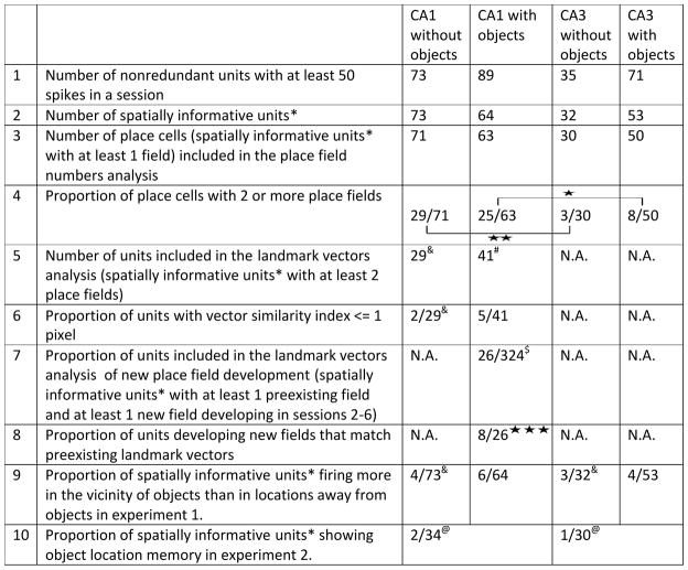
Summary of number of neurons included in different analyses and proportions of neurons passing the threshold of significance in the given analysis.

^*Spatially informative units were defined as those that fired ≥ 50 spikes/session, had a statistically significant (p < 0.01) spatial information score > 0.25bits/spike.

^★ p < 0.05;

^★★p < 0.01;

^★★★p <0.001.

^# 25 of the 63 nonredundant cells meeting criteria for having at least 1 field in CA1 have two or more fields; however, since we are interested in cells with at least 2 fields for the landmark vector analysis, we repeated the redundancy elimination process (see results) for units with at least 2 fields (instead of redundancy elimination over the entire population) in CA1 with objects condition. This yielded 41 units in this condition.

^$ 324 neurons with spatial information score > 0.25 bits/spike were recorded from CA1 in the presence of objects, over the course of experiment 1. Only subsets of these neurons were included in various analyses because of possible redundancy across days.

^@ Experiment 2 had without object sessions at the beginning and end of the day, and intervening sessions had one object at different locations.

^& As a control, landmark vector (rows 5,6) and object responsiveness (row 9) analyses were also performed on without-object sessions that were recorded before the introduction of objects. The standard locations of objects from the with-object sessions that followed the without-object sessions were used in these analyses. These controls serve as a measure of probability that the observed proportion of responsive neurons is a chance phenomenon.

Figure 3. Comparison of number of place fields in CA1 and CA3.

CA1 neurons have more place fields on an average than CA3 neurons, both in the presence and absence of objects.

Landmark vector cells

Some of the neurons with two or more place fields in CA1 showed an apparently nonrandom distribution of place fields. These place fields were located such that vectors connecting at least two place fields to two objects were nearly identical (Figure 4A), indicating that these fields may be encoding the two spatial locations independently in relation to two objects. For neurons with two or more place fields (Table 1, line 4), the probability of obtaining such nearly identical landmark vectors was quantified using a randomization protocol (see methods). For each cell, a vector was calculated between each of its place fields and the locations of each object in the environment (or in the case of without-objects sessions, with the locations that each object occupied in the subsequent with-objects sessions). The two most similar vectors that did not share an object or a place field were identified, and a LV similarity index was calculated by subtracting one of these vectors from the other. In the absence of objects, as expected, the distribution of LV similarity indices was not statistically distinguishable from the randomized distribution (Figure 4B; n = 29, median = 5.55 pixels, IQRB = 3.72 – 7.61 pixels; randomized n = 29, median = 6.25pixels, IQRB = 3.80 – 9.51 pixels; p = 0.52). In contrast, in the presence of objects, the distribution of vector differences between the two most similar LVs was significantly smaller than the corresponding randomized distribution (Figure 4B; n= 41, median = 4.74 pixels, IQRB = 2.20 – 8.40 pixels; randomized n = 41, median = 6.25 pixels, IQRB = 3.93 – 9.51 pixels; Wilcoxon ranksum test, p = 0.0194), suggesting that more LVs were similar to each other than expected by chance. Indeed, the mode of the distribution of the experimental data with objects was the 0–0.5 pixel bin (red arrow in figure 4B), indicating that the most common vector difference was <1 pixel (i.e., the vectors were nearly identical). When comparing the data distributions with and without objects directly, however (Fig. 4B, top row), the vector difference between the two most similar LVs was not significantly different (p = 0.38), perhaps due to the small numbers of cells available for this analysis (i.e., those showing multiple fields).

Figure 4. Landmark vector cells.

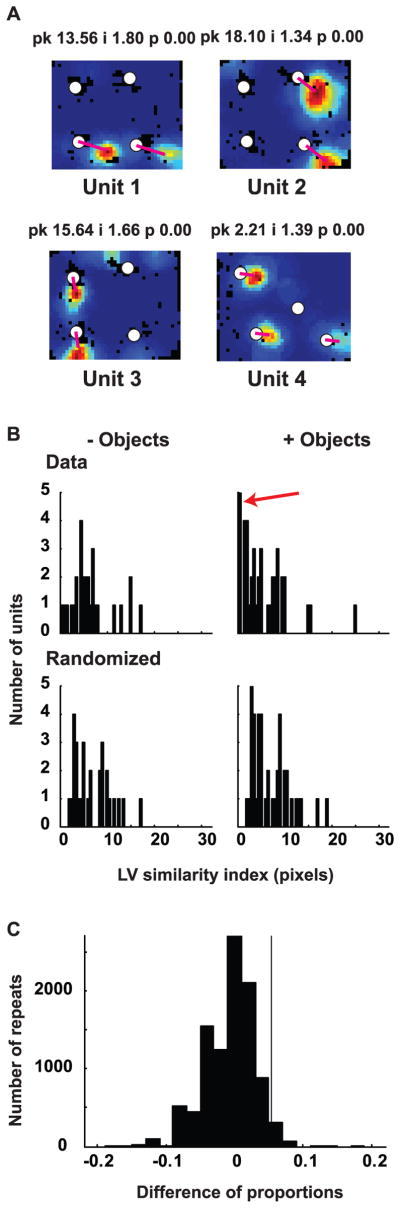
(A) Examples of CA1 neurons with two or three fields with matching LVs. Magenta lines connect objects with place fields to indicate similarity of the LVs. (B) Distribution of LV similarity indices (vector differences between the most similar LVs) in CA1 in the presence and absence of objects. Histograms at the top are for the actual data, while those at the bottom are for the corresponding randomized distributions with equal number of units as the actual data. Notice the highly skewed distribution of observed data in the presence of objects. The red arrow in the with-objects condition marks the large number of neurons with a LV similarity index in the 0–0.5 pixel bin. (C) Expected distribution of the difference in proportion of neurons with a LV similarity index < 1 pixel between with-objects (41 samples) and without-objects (29 samples) conditions as estimated by resampling from randomized data (see methods). The vertical line marks the position of the observed difference of proportions, indicating that it lies on the positive tail of the expected distribution.

Identical LVs should have a LV similarity index value < 1 pixel (i.e., the resolution of the spatial rate maps). To overcome the limitations of the small sample size, we compared the difference in the proportion of neurons with LV similarity index < 1 pixel between the data with (5/41) and without (2/29) objects (Table 1, lines 5–6) to a simulated randomized distribution of this difference. To create this distribution, we created 10,000 pairs of randomized distributions with the same number of units as the pair of randomized distributions in Figure 4B, drawing with replacement from a pool of 100,000 randomized rate maps for each rat (created as described in the Methods). For each pair, we calculated the difference in the proportions of LV similarity index < 1 pixel to obtain a distribution of the expected value of this difference (i.e., 0) under the assumption that both distributions were identical. Figure 4C shows that the observed difference (5/41 – 2/29 = 0.053; black line in Fig. 4C) was significantly larger than that expected by chance (p = 0.039), supporting the conclusion that the with-object condition had significantly higher proportion of neurons with nearly identical LVs than the without-object condition.

The most powerful evidence for the existence of landmark vector cells comes from an analysis of the neurons that developed new place fields during the course of a day’s recordings. Twenty six CA1 place cells developed new place field(s) in addition to preexisting field(s) (Table 1, line 7). Were these new fields more likely than chance to match the LV relationship of the prior field(s)? The LV similarity index for each of the neurons developing new fields was compared with the corresponding distribution of randomized LV similarity indices to estimate the probability of obtaining the observed LV similarity index by chance (see methods). A higher proportion of neurons (8/26; Table 1, line 8) had statistically significant LV indices (p < 0.05) than expected by chance at an alpha level of 0.05 (test for proportions 8/26 vs. 1/20, z = 6.03, p ≪ 10⁻⁵; Figure 5 and unit 5 in Figure 2). Of these 8 neurons, two neurons with two matching LVs developed a third LV in the course of recordings that matched the two preexisting LVs (Figure 5, Units 6 and 7), while a third neuron developed two new fields over multiple sessions, matching the LV of the first field (Figure 2, unit 5). Another 5 CA1 neurons developed a second field matching the LV of a preexisting field (Figure 5, units 1–5).

Figure 5. Neurons developing new LV(s) matching preexisting LV(s).

Eight CA1 neurons developed new field(s) that fired at a spatial location with a LV matching a preexisting LV. Units 1–5 developed a second LV. Unit 6 developed a third LV matching the previous two. Unit 7 developed a fourth LV, however, one of the preexisting LVs moved away from its original location at the same time. See also unit 5 in figure 2, which started out with a single field, but over the course of 6 sessions, developed two more fields matching the LV of the first field.

We further tested the significance of the landmark vector results in these 26 neurons by comparing the LV similarity index with indices that would arise from other hypothetical relationships between the landmarks and the place fields. One hypothetical relationship is that for a cell with two place fields, the LVs of the fields would be of equal length but opposite orientation. Another hypothetical relationship is that for a cell with three place fields, the LVs of the fields would have similar lengths but be oriented 120° apart. If there were no tendency for LVs to be similar in both length and orientation, then the numbers of neurons showing these alternative hypothetical relationships should be as prevalent as those showing the matching LVs relationship. For the 2 matching LV scenario, the LV similarity index was calculated for the observed as well as randomized data after the second vector of a pair was rotated by 180°. For the 3 matching LV scenario, the LV similarity index was calculated for the observed as well as randomized data after the second vector was rotated by 120° and the third vector was rotated by 240°. None of the 26 neurons showed statistically significant (p < 0.05) LV similarity indices either for two LVs with opposite orientation and similar length, or for three LVs with orientations spaced 120° apart and similar length. Thus the proportion of neurons with matching LVs (8/26) was significantly higher than the proportion of neurons with arbitrarily defined LV relationships (0/26; χ² = 7.24, p = 0.0071). The low probability of obtaining the observed configurations by chance coupled with the fact that this proportion is higher than a proportion of neurons with other defined LV relationships support the hypothesis that these neurons encode spatial locations in relation to individual landmarks at a high level of accuracy. Furthermore, the formation of new fields with new LVs matching preexisting LVs also indicates that the landmark vector relationships are dynamically encoded, and at least some neurons in CA1 may be capable of transferring vector relationships from one landmark to another.

Influences of Head Direction, Experience, Anatomical Location, and Individual Rat Differences

It is of considerable interest to know whether the landmark-vector responses reported here are dependent on such factors as the animal’s head direction, experience with the objects, anatomical location along the proximal-distal axis of CA1, and individual differences. Unfortunately, we cannot answer any of these questions with precision, based on the small numbers of cells that show these properties and the limited sampling of head directions within each subfield. Nonetheless, we provide here some anecdotal information that is relevant to these questions. We purposely refrain from giving specific numbers, as these would likely be inaccurate and potentially misleading indicators of the magnitudes of any potential effects.

Head Direction

It is important to know whether the landmark vector cells fire when the rat is facing all head directions, or whether the firing is limited to a single direction (implying a potential egocentric component to the responses). Because the sessions were limited typically to 15 min duration and the recording environment was large, we were unable to obtain complete, uniform sampling of all head directions within each subfield of the landmark vector cells. Movement biases of the rats, especially along the environment boundaries, compounded this problem. Thus, we cannot address this question with certainty. However, we inspected the firing of the landmark vector cells as a function of head direction and observed no strong evidence that the cells were strongly, directionally modulated. For example, most of the subfields showed firing when the rat passed through the field in at least 2 orthogonal directions. Furthermore, any potential directional tuning within a subfield typically was not matched by the tuning in other subfields of that cell. Thus, although it is possible that the cells have directional biases, these biases were not strong enough to show obvious directional tuning within the constraints of the sampling problems of the present study. A definitive answer will require an experiment in which the recording sessions are much longer in order to overcome these directional sampling issues.

Experience

Examples of landmark vector cells were seen on the very first day with objects (for example, unit 1 of Figure 5) as well as on subsequent days. Thus, although the development of subfields that match previous vectors clearly shows some degree of experience dependence, it is not known whether all landmark vector fields develop over time or whether there is a bias for the proportion of landmark vector cells to increase with the animal’s experience with the objects.

Anatomical location

Because proximal CA1 is preferentially connected with MEC and distal CA1 is preferentially connected with LEC (Witter and Amaral, 2004) it is important to know whether the landmark vector cells are differentially distributed along the proximal-distal axis. Two rats had tetrode bundles in the proximal half of CA1 and two rats had tetrode bundles in the distal half of CA1. We observed examples of landmark vector cells from recording sites in both the proximal and distal halves of CA1. Thus, it is unlikely that there is an absolute distinction between the two regions. However, there may be biases in the prevalence of these properties along the proximal-distal axis that will require a larger data set to quantify.

Individual Differences

We have seen examples of landmark vector properties in all 4 of the rats in this study. Although the landmark vector cells analyzed quantitatively in this report did not come from all rats (based on the independent methods we used to select individual data sets in order to remove neurons potentially recorded over multiple days), we saw clear examples of these phenomena in some sessions in all 4 rats. Across all days of recordings, we saw no evidence of strong differences in the proportions of landmark vector cells across the 4 rats. The proportions of LV cells to total number of cells with 2 or more fields, averaged over 5 days of recordings, were as follows: rat 1: 1.33/5.33, rat 2: 2/5, rat 3: 3.75/19.5, and rat 4: 1.4/8.6.

Object location memory and object selectivity

We next tested whether CA1 and CA3 place fields were more likely than chance to be located right next to the objects, potentially reflecting the object-related firing properties of hippocampal inputs from the LEC and perirhinal cortex (Deshmukh and Knierim, 2011; Deshmukh et al., 2012; Burke et al., 2012). In order to test if an increased proportion of neurons fire at object locations in the presence of objects, the proportion of neurons firing near object locations before the introduction of objects was compared to the proportion of neurons firing near objects in their presence. Only neurons with statistically significant (p < 0.01) spatial information scores > 0.25 bits/spike were included in this analysis, to avoid false positive responses.

In the absence of objects, 4/73 CA1 neurons fired preferentially around locations where the objects were to be placed in the following session (i.e. had p_min(ORI) < 0.05). In comparison, 6/64 CA1 neurons recorded in presence of objects did the same (χ² = 0.3, p = 0.59). Similarly, the proportion of neurons firing preferentially around objects in CA3 did not differ in with and without objects conditions (without objects: 3/32 units; with objects: 4/53 units; χ² = 0.01 p = 0.91; Table 1, line 9). Thus, the presence of objects did not induce a larger proportion of CA1 or CA3 neurons to fire at the object locations under the current experimental conditions.

Although in our experiment few neurons responded preferentially to object locations per se, we did detect an instance in which a CA3 neuron showed a “memory” for object location when the object was removed (Figure 6, Unit 1). This unit did not fire at familiar objects, even when one of them was moved in session 3. In session 5, when a novel object was introduced, this neuron developed a field at the novel object, and continued firing robustly at this location even after the object was removed in session 6. Thus this neuron may be responding to object identity/novelty or object + place conjunction in session 5, and has correlates of object location memory in session 6. This firing property is similar, if not identical, to the “misplace cell” activity reported by O’Keefe (1976). To gain further insight into this phenomenon, we performed an additional experiment on 2 of the rats. In experiment 2, two rats foraged in a square box for chocolate sprinkles. There were no objects in the first and last session, while in the intervening 3 sessions, one object was placed at three different locations in each session. This protocol provided more opportunities than Experiment 1 for testing object + location correlates as well as activity related to object location memory. Unit 2, recorded from CA3, did not fire at the object in session 2, but it fired at the locations where the object used to be in the subsequent sessions. This unit fired at the object location in session 4, but this field was weaker than the other two fields at locations where the object used to be in sessions 2 and 3. In session 5, the unit had three fields corresponding to the three locations of the object in previous sessions. In addition, over the course of sessions, a strong place field present in session 1 shifted toward the nearest object location. Thus this neuron had correlates of object location memory which lasted over multiple sessions. Unit 3, recorded from CA1, did not fire at the object in session 2, but when the object was moved to a new location in session 3, the unit fired at the previous location occupied by the object in session 2. This field remained in the rest of the sessions, including weakly in session 5 when there were no objects in the environment. The neuron did not do the same at other locations that the same object was encountered in sessions 3 and 4. Thus, this neuron encoded a memory of a specific object + place combination. Unit 4, recorded from CA1 on the second day, had fields at two of the locations where the object had been placed on day 1, as well as a few spikes near the third location where the object had been placed on day 1 (white circles in session 1 indicate locations where an object had been placed on day 1 in three different sessions). This pattern in session 1 indicated that this neuron had a memory of object locations from the previous day. In session 2, when an object (different from the object used on day 1) was placed at a location of a preexisting field, the neuron fired less at that location, but had a new field that stretched from the object location on day 1 session 2 toward the current location of the different object. In session 3, this neuron fired at all three object locations, including the current location of the object, as well as at a point between the other two object locations. In session 4, the neuron did not fire at the present location of the object, but did so at the other locations where the object had been. In session 5, this neuron continued firing at object locations, even when there were no objects in the environment. Thus, this neuron had correlates of object location memory at multiple locations of the objects, which lasted for (at least) a day. Unit 5 fired less than 50 spikes in sessions 1–3. This neuron fired at the location of the object in all sessions with the object, and most of these spikes occurred during a single pass of the rat by the object (resulting in statistically insignificant but high spatial information scores). Thus this neuron responded to the object, albeit weakly, irrespective of its location. All other neurons in this figure met the criteria for minimum number of spikes and spatial information score previously used for object-responsive neurons. Unit 6 did not fire at the object in session 2, but fired at the same object at a different location in session 3. Unlike unit 5, this unit fired at the object in multiple passes in session 3. In session 4, the object was placed at a location that already had a field from session 2; this field continued to be at the same location even in the presence of the object (though the peak firing rate nearly doubled). Given the lack of response to the object in session 2, the response to the same object in session 3 can be interpreted as an object + place conjunctive response.

Figure 6. Neuronal responses to object manipulations.

Unit 1 was recorded in experiment 1, while units 2 – 6 were recorded in experiment 2. Standard objects in experiment 1 are marked as filled white circles. The object that changed location from session to session in experiment 2 and the misplaced and novel objects in experiment 1 are marked as white stars. Open white circles in unit 4 session 1 mark the location where a different object was placed in sessions 2–4 of the previous day. The magenta line connects the standard location of the misplaced object with its misplaced location in session 3, for unit 1.

Similar to experiment 1, only a small proportion of neurons showed object related activity in experiment 2. Thirty four CA1 neurons and 30 CA3 neurons met the criteria for inclusion in the quantitative analyses for at least one session (firing at least 50 spikes in the given session and having statistically significant (p < 0.01) spatial information scores > 0.25 bits/spike). Of these, 2 CA1 neurons and 1 CA3 neuron showed object location memory (Table 1, line 10), 2 CA1 neurons showed object + place conjunctive responses and 1 CA1 neuron fired at the object irrespective of its spatial location.

Discussion

Object location memory

Some neurons in the present study increased firing at spatial locations where an object used to be. Such correlates of object location memory have been demonstrated previously in the hippocampus (O’Keefe, 1976), the anterior cingulate cortex (Weible et al., 2009) and the lateral entorhinal cortex (Deshmukh and Knierim, 2011; Tsao et al., 2011). This object + place conjunctive activity lasts over multiple sessions, and in the case of one neuron, overnight, in the present study. In the anterior cingulate cortex (Weible et al., 2012) and the lateral entorhinal cortex (Tsao et al., 2011), the object location memory responses have been shown to last over a number of days, indicating that the hippocampal system is capable of retaining memory of object locations for prolonged periods of time, as envisaged by the cognitive map theory (O’Keefe and Nadel, 1978). One caveat to consider is whether the putative memory responses are actually sensory responses to cues left behind (e.g., odors) when the objects were moved. Can the apparent object location memory be explained in terms of sensory responses to odors left behind by objects? In sessions where the object was still present in the environment, the object at its current location would be a stronger source of the object-odor than the previous location of the object. If the neurons were merely responding to the object-odor, the response would be expected to be as strong, if not stronger, at the current location of the object than the past location(s) of the object. We observed units in the hippocampus that fire much more at location(s) where the object used to be, rather than where it currently is (Figure 6 units 2, 3). Thus, the observed object location memory correlates cannot be explained in terms of purely sensory phenomena, although we cannot definitely rule out the potential contribution of such influences.

Landmark vectors

McNaughton et al. (1995) proposed a vector representation model wherein place fields were hypothesized to represent a vector, with a bearing set by the head direction system (Taube et al., 1990; Yoganarasimha et al., 2006) and a length determined by a distance from a landmark. In a given environment, place cell vectors were hypothesized to be bound to one or more landmarks [“typically one, occasionally two, rarely more than two”; (McNaughton et al., 1995), p. 591]. Assuming that each cell encodes only one distance-bearing pair, they predicted that neurons bound to two or more landmarks would fire at as many locations, which have matching distance-bearing relationships with those landmarks. To our knowledge, the neurons with two or more matching LVs shown in this paper are a first demonstration of this binding of spatial representation to multiple, discrete landmarks, although a similar binding to multiple environmental boundaries has been previously demonstrated (Burgess et al., 2000; Hartley et al., 2000; Solstad et al., 2008; Lever et al., 2009 ). The neurons with matching LVs in the present study may be an underestimate of the true number of landmark-vector encoding cells. Under the current experimental conditions, neurons with single place fields anchored to individual landmarks cannot be distinguished from those representing spatial locations in a global reference frame. This excludes a majority of CA1 neurons and almost all CA3 neurons from the current analysis of the landmark vector phenomenon. Hence, this report should not be interpreted as claiming either that neurons with single place fields do not encode landmark vectors or that CA3 does not have landmark vector representation; we are unable to make any claims regarding either of these questions. Furthermore, the cells with multiple fields that do not have matching LVs may also be encoding spatial locations as distances and bearings from some uncontrolled landmarks (e.g. corners, local textures, odors etc).

Boundary vector cells and landmark vector cells

O’Keefe and Burgess (1996) hypothesized the existence of boundary vector cells in a model of the influence of the apparatus boundaries on place cell firing. Cells firing parallel to environmental boundaries were later shown to be present in the medial entorhinal cortex, the parasubiculum and the subiculum (Solstad et al., 2008; Savelli et al., 2008; Lever et al., 2009; Boccara et al., 2010), matching the prediction of boundary vector cells. The boundary vector cell model defined the boundary vector cells in terms of distance and direction from a boundary (Burgess et al., 2000; Hartley et al., 2000). This model is similar to the vector representation model (McNaughton et al., 1995), except that the vectors are anchored to the boundaries instead of more discrete landmarks. As a consequence of the reference being a line in the case of boundary vector cell model, as opposed to a point in the landmark vector model, the boundary vector cells have fields that run parallel to the boundaries, while landmark vector cells fire at a unique spatial location. Thus, the landmark vector cells reported here may be functionally equivalent to boundary vector cells, the difference being the category of external landmarks to which the vector is bound.

Landmark vectors as reference frames

A landmark vector is defined in terms of distance and orientation with respect to a landmark. This is a classic definition of a reference frame. However, the cells with multiple matching LVs indicate that there are multiple competing ‘origins’ for these reference frames, for individual neurons in the hippocampus. While such a redundancy in the number of origins (and hence number of reference frames) creates an ambiguity about spatial location encoded by a single neuron (e.g. when unit 2 in Figure 4A fires, the rat could either be 5 pixels southeast of one object or another), it is by no means the only example of such ambiguity in the activity of a single hippocampal neuron. For example, boundary vector cells are predicted to fire at a specific distance and orientation from a boundary (Burgess et al., 2000; Hartley et al., 2000). These cells maintain the same relationship with a pair of parallel boundaries in the environment, thus firing along two parallel lines (Solstad et al., 2008; Lever et al., 2009). Some place cells, thought to be created by summation of overlapping boundary vector cell inputs (Burgess et al., 2000; Hartley et al., 2000) also show a corresponding redundancy in spatial firing. When there are two parallel walls in the environment, the hippocampus has place cells that fire at two locations, identical in terms of distance and location along the two parallel boundaries, as predicted by the boundary vector cell model (Hartley et al., 2000). Similarly, when the rats run on a spiral track, hippocampal neurons fire at multiple locations on the spiral. For the given neuron, the spatial location of firing in each lap of the spiral matches with that in the other laps (Nitz, 2011; see also Hayman et al., 2011).

Of what use are these landmark vector cells that fire at a fixed distance and orientation from two or more objects? Would such a redundancy not hamper rather than enhance the rat’s ability to navigate? One possibility is that the landmark vector cells encode distance and orientation from specific features on the landmarks (McNaughton et al., 1995). In this formulation, while most landmark vector cells will encode distance and orientation from unique landmarks, occasionally two or more landmarks may share a feature that causes a landmark vector cell to fire at multiple locations. Thus, the landmark vector cells with multiple LV fields might be a consequence of the underlying LV computation (that serendipitously helps us in detection of landmark vector cells), but may not be computationally advantageous. Alternatively, the behavioral demands of the task might determine whether the landmark vector cells generalize distance and orientation from multiple landmarks or fire at unique locations defined with respect to single landmarks. In the present experiment, the rats were foraging for chocolate sprinkles in the presence of multiple objects. These objects were not navigationally significant in terms of indicating a path to a goal, but may have been perceived as obstacles to be avoided while foraging. Landmark vector cells that do not discriminate between the objects while encoding distances and directions from these objects might play a crucial role in avoidance of these obstacles. A corollary of this hypothesis would be that the landmark vector cells should not generalize when the objects in the environment are being used for navigation. It will be impossible to find landmark vector cells under these conditions using the methods used in this paper.

General conclusions

Place fields are often discussed as if they represent a unitary phenomenon, created by a single mechanism. Although conclusive evidence has demonstrated that the hippocampal representations of space can be dissociated into separate frames of reference (Gothard et al., 1996a,b; Zinyuk et al., 2000; Knierim, 2002; Lee et al., 2004), these dissociations do not necessarily entail distinct mechanisms of the formation of spatial firing. Rivard et al. (2004) showed evidence that there were at least two classes of place cells, one class that signals proximity to a barrier and another that signals location in an allocentric reference frame. Other studies have shown that hippocampal cells respond to objects and object manipulations in various ways. For example, objects located at the periphery of the arena, but not those located near the center, control place cell firing (Cressant et al., 1997; Cressant et al., 1999); objects located at the periphery of the arena exert stronger control over place cell firing than distal cues (Renaudineau et al., 2007); and firing rates of hippocampal neurons are modulated within their place fields by objects (Manns and Eichenbaum, 2009; Komorowski et al., 2009). Inspection of rate maps in circular environments demonstrates clear heterogeneity in the shapes of place fields, with crescent-shaped fields tending to form along the walls and circular fields in the middle of the environment. It is becoming increasingly clear that cells in the hippocampal afferent structures (the LEC and MEC) have a diverse set of properties, including grid cell activity patterns, boundary-related activity, and object-related activity. It thus seems likely that the spatial firing patterns of hippocampal place cells arise from a combination of different inputs. Place fields may arise from differing combinations of input from grid-cells (de Almeida et al., 2009; Solstad et al., 2006; Savelli and Knierim, 2010; Monaco and Abbott, 2011) and boundary cells (Burgess et al., 2000; Hartley et al., 2000) of the MEC and object-based spatial representations of the LEC (Deshmukh and Knierim, 2011). Thus, the crescent shaped place field in the hippocampus may arise primarily from boundary-cell inputs, circular fields in the center of an apparatus may arise from grid cell inputs, fields in the corners may arise from corner-responsive neurons ( Savelli and Knierim, 2010; Deshmukh and Knierim, 2011), and landmark vector cells may arise from object representations and object-based spatial representations of the LEC in conjunction with path integration-based inputs (such as representations of head direction and distance) from MEC.

It is also important to consider whether the different response types of hippocampal cells imply distinct “classes” of cells, or whether the responses are merely variations along a continuum of responses that depend on the precise sets of inputs that are active upon a cell at a particular time or in a particular context. Specifically, should the landmark vector cells reported here be considered a class of cells distinct from standard place cells? In the absence of corroborating evidence, we would caution against such a conclusion. It is possible that these cells would show standard place fields under other conditions. For example, Gothard et al. (1996b) showed that place cells that were bound to a start box reference frame under one set of experimental conditions acted as standard place cells under a different set of conditions. It is possible that the landmark vector cells are similar in properties to most place cells, but that they represent a minority of cells that become bound to landmarks in ways that are similar to place fields becoming “bound” to other sensory or cognitive inputs. Thus, place cells, misplace cells (O’Keefe, 1976), time/sequence cells (Pastalkova et al., 2008; McDonald et al., 2011), splitter cells (Wood et al., 2000), barrier cells (Rivard et al., 2004), and landmark vector cells (to name a subset of hippocampal responses) may show different phenomenology depending on experimental conditions, but they may still reflect the same underlying computational processes performed on different, dynamically changing, inputs. If one were to correlate specific properties with other independent differences in pyramidal cells (such as differences in cellular morphology, anatomical location, connectivity, gene expression, or cellular physiology; Mizuseki et al., 2011; Lein et al., 2007; Senior et al., 2008; Graves et al., 2012), then a stronger case can be made that different response types correspond to distinct cell classes. In the absence of such independent evidence, use of terms such as landmark vector cells, time cells, splitter cells, and misplace cells should be taken as descriptions of different types of responses of a possibly single underlying class of cells, rather than as distinct classes of cells.

References

- Aggleton JP, Brown MW. Episodic memory, amnesia, and the hippocampal-anterior thalamic axis. Behav Brain Sci. 1999;22:425–444. [PubMed] [Google Scholar]
- Boccara CN, Sargolini F, Thoresen VH, Solstad T, Witter MP, Moser EI, Moser MB. Grid cells in pre- and parasubiculum. Nat Neurosci. 2010;13:987–994. doi: 10.1038/nn.2602. [DOI] [PubMed] [Google Scholar]
- Burgess N, Jackson A, Hartley T, O’Keefe J. Predictions derived from modelling the hippocampal role in navigation. Biol Cybern. 2000;83:301–312. doi: 10.1007/s004220000172. [DOI] [PubMed] [Google Scholar]
- Burke SN, Maurer AP, Hartzell AL, Nematollahi S, Uprety A, Wallace JL, Barnes CA. Representation of three-dimensional objects by the rat perirhinal cortex. Hippocampus. 2012;22:2032–2044. doi: 10.1002/hipo.22060. [DOI] [PMC free article] [PubMed] [Google Scholar]
- Collett TS, Cartwright BA, Smith BA. Landmark learning and visuo-spatial memories in gerbils. J Comp Physiol A. 1986;158:835–851. doi: 10.1007/BF01324825. [DOI] [PubMed] [Google Scholar]
- Cressant A, Muller RU, Poucet B. Failure of centrally placed objects to control the firing fields of hippocampal place cells. J Neurosci. 1997;17:2531–2542. doi: 10.1523/JNEUROSCI.17-07-02531.1997. [DOI] [PMC free article] [PubMed] [Google Scholar]
- Cressant A, Muller RU, Poucet B. Further study of the control of place cell firing by intra- apparatus objects. Hippocampus. 1999;9:423–431. doi: 10.1002/(SICI)1098-1063(1999)9:4<423::AID-HIPO8>3.0.CO;2-U. [DOI] [PubMed] [Google Scholar]
- de Almeida L, Idiart M, Lisman JE. The input-output transformation of the hippocampal granule cells: from grid cells to place fields. J Neurosci. 2009;29:7504–7512. doi: 10.1523/JNEUROSCI.6048-08.2009. [DOI] [PMC free article] [PubMed] [Google Scholar]
- Deshmukh SS, Johnson JL, Knierim JJ. Perirhinal cortex represents nonspatial, but not spatial information in rats foraging in the presence of objects: comparison with lateral entorhinal cortex. Hippocampus. 2012;22:2045–2058. doi: 10.1002/hipo.22046. [DOI] [PMC free article] [PubMed] [Google Scholar]
- Deshmukh SS, Knierim JJ. Representation of non-spatial and spatial information in the lateral entorhinal cortex. Front Behav Neurosci. 2011;5:69. doi: 10.3389/fnbeh.2011.00069. [DOI] [PMC free article] [PubMed] [Google Scholar]
- Deshmukh SS, Yoganarasimha D, Voicu H, Knierim JJ. Theta modulation in the medial and the lateral entorhinal cortices. J Neurophysiol. 2010;104:994–1006. doi: 10.1152/jn.01141.2009. [DOI] [PMC free article] [PubMed] [Google Scholar]
- Fox SE, Ranck JB. Electrophysiological characteristics of hippocampal complex-spike cells and theta cells. Exp Brain Res. 1981;41:399–410. doi: 10.1007/BF00238898. [DOI] [PubMed] [Google Scholar]
- Frank LM, Brown EN, Wilson MA. A comparison of the firing properties of putative excitatory and inhibitory neurons from CA1 and the entorhinal cortex. J Neurophysiol. 2001;86:2029–2040. doi: 10.1152/jn.2001.86.4.2029. [DOI] [PubMed] [Google Scholar]
- Gothard KM, Skaggs WE, Moore KM, McNaughton BL. Binding of hippocampal CA1 neural activity to multiple reference frames in a landmark-based navigation task. J Neurosci. 1996a;16:823–835. doi: 10.1523/JNEUROSCI.16-02-00823.1996. [DOI] [PMC free article] [PubMed] [Google Scholar]
- Gothard KM, Skaggs WE, Moore KM, McNaughton BL. Binding of hippocampal CA1 neural activity to multiple reference frames in a landmark-based navigation task. J Neurosci. 1996b;16:823–835. doi: 10.1523/JNEUROSCI.16-02-00823.1996. [DOI] [PMC free article] [PubMed] [Google Scholar]
- Graves AR, Moore SJ, Bloss EB, Mensh BD, Kath WL, Spruston N. Hippocampal Pyramidal Neurons Comprise Two Distinct Cell Types that Are Countermodulated by Metabotropic Receptors. Neuron. 2012;76:776–789. doi: 10.1016/j.neuron.2012.09.036. [DOI] [PMC free article] [PubMed] [Google Scholar]
- Hartley T, Burgess N, Lever C, Cacucci F, O’Keefe J. Modeling place fields in terms of the cortical inputs to the hippocampus. Hippocampus. 2000;10:369–379. doi: 10.1002/1098-1063(2000)10:4<369::AID-HIPO3>3.0.CO;2-0. [DOI] [PubMed] [Google Scholar]
- Hayman R, Verriotis MA, Jovalekic A, Fenton AA, Jeffery KJ. Anisotropic encoding of three-dimensional space by place cells and grid cells. Nat Neurosci. 2011;14:1182–1188. doi: 10.1038/nn.2892. [DOI] [PMC free article] [PubMed] [Google Scholar]
- Holm S. A simple sequential rejective multiple test procedure. Scandinavian Journal of Statistics. 1979;6:65–70. [Google Scholar]
- Knierim JJ. Dynamic interactions between local surface cues, distal landmarks, and intrinsic circuitry in hippocampal place cells. J Neurosci. 2002;22:6254–6264. doi: 10.1523/JNEUROSCI.22-14-06254.2002. [DOI] [PMC free article] [PubMed] [Google Scholar]
- Knierim JJ, Hamilton DA. Framing Spatial Cognition: Neural representations of proximal and distal frames of reference and their roles in navigation. 2011. p. 1279. [DOI] [PMC free article] [PubMed] [Google Scholar]
- Knierim JJ, Lee I, Hargreaves EL. Hippocampal place cells: parallel input streams, subregional processing, and implications for episodic memory. Hippocampus. 2006;16:755–764. doi: 10.1002/hipo.20203. [DOI] [PubMed] [Google Scholar]
- Knierim JJ, Rao G. Distal landmarks and hippocampal place cells: effects of relative translation versus rotation. Hippocampus. 2003;13:604–617. doi: 10.1002/hipo.10092. [DOI] [PubMed] [Google Scholar]
- Komorowski RW, Manns JR, Eichenbaum H. Robust conjunctive item-place coding by hippocampal neurons parallels learning what happens where. J Neurosci. 2009;29:9918–9929. doi: 10.1523/JNEUROSCI.1378-09.2009. [DOI] [PMC free article] [PubMed] [Google Scholar]
- Lee I, Yoganarasimha D, Rao G, Knierim JJ. Comparison of population coherence of place cells in hippocampal subfields CA1 and CA3. Nature. 2004;430:456–459. doi: 10.1038/nature02739. [DOI] [PubMed] [Google Scholar]
- Lein ES, Hawrylycz MJ, Ao N, Ayres M, Bensinger A, Bernard A, Boe AF, Boguski MS, Brockway KS, Byrnes EJ, et al. Genome-wide atlas of gene expression in the adult mouse brain. Nature. 2007;445:168–176. doi: 10.1038/nature05453. [DOI] [PubMed] [Google Scholar]
- Lever C, Burton S, Jeewajee A, O’Keefe J, Burgess N. Boundary vector cells in the subiculum of the hippocampal formation. J Neurosci. 2009;29:9771–9777. doi: 10.1523/JNEUROSCI.1319-09.2009. [DOI] [PMC free article] [PubMed] [Google Scholar]
- Manns JR, Eichenbaum H. A cognitive map for object memory in the hippocampus. Learn Mem. 2009;16:616–624. doi: 10.1101/lm.1484509. [DOI] [PMC free article] [PubMed] [Google Scholar]
- MacDonald CJ, Lepage KQ, Eden UT, Eichenbaum H. Hippocampal “time cells” bridge the gap in memory for discontiguous events. Neuron. 2011;71:737–749. doi: 10.1016/j.neuron.2011.07.012. [DOI] [PMC free article] [PubMed] [Google Scholar]
- McNaughton BL, Knierim JJ, Wilson MA. Vector encoding and the vestibular foundations of spatial cognition: neurophysiological and computational mechanisms. In: Gazzaniga MS, editor. The cognitive neurosciences. Cambridge, Mass: MIT Press; 1995. pp. 585–595. [Google Scholar]
- Mizuseki K, Diba K, Pastalkova E, Buzsaki G. Hippocampal CA1 pyramidal cells form functionally distinct sublayers. Nat Neurosci. 2011;14:1174–1181. doi: 10.1038/nn.2894. [DOI] [PMC free article] [PubMed] [Google Scholar]
- Moita MA, Rosis S, Zhou Y, LeDoux JE, Blair HT. Hippocampal Place Cells Acquire Location-Specific Responses to the Conditioned Stimulus during Auditory Fear Conditioning. Neuron. 2003;37:485–497. doi: 10.1016/s0896-6273(03)00033-3. [DOI] [PubMed] [Google Scholar]
- Monaco JD, Abbott LF. Modular realignment of entorhinal grid cell activity as a basis for hippocampal remapping. J Neurosci. 2011;31:9414–9425. doi: 10.1523/JNEUROSCI.1433-11.2011. [DOI] [PMC free article] [PubMed] [Google Scholar]
- Nitz DA. Path shape impacts the extent of CA1 pattern recurrence both within and across environments. J Neurophysiol. 2011;105:1815–1824. doi: 10.1152/jn.00573.2010. [DOI] [PubMed] [Google Scholar]
- O’Keefe J. Place units in the hippocampus of the freely moving rat. Exp Neurol. 1976;51:78–109. doi: 10.1016/0014-4886(76)90055-8. [DOI] [PubMed] [Google Scholar]
- O’Keefe J, Burgess N. Geometric determinants of the place fields of hippocampal neurons. Nature. 1996;381:425–428. doi: 10.1038/381425a0. [DOI] [PubMed] [Google Scholar]
- O’Keefe J, Dostrovsky J. The hippocampus as a spatial map: Preliminary evidence from unit activity in the freely-moving rat. Brain Res. 1971;34:171–175. doi: 10.1016/0006-8993(71)90358-1. [DOI] [PubMed] [Google Scholar]
- O’Keefe J, Nadel L. The hippocampus as a cognitive map. Oxford: Clarendon Press; 1978. [Google Scholar]
- Pastalkova E, Itskov V, Amarasingham A, Buzsáki G. Internally generated cell assembly sequences in the rat hippocampus. Science. 2008;321:1322–1327. doi: 10.1126/science.1159775. [DOI] [PMC free article] [PubMed] [Google Scholar]
- Ranck JB. Studies on single neurons in dorsal hippocampal formation and septum in unrestrained rats. I. Behavioral correlates and firing repertoires. Exp Neurol. 1973;41:461–531. doi: 10.1016/0014-4886(73)90290-2. [DOI] [PubMed] [Google Scholar]
- Renaudineau S, Poucet B, Save E. Flexible use of proximal objects and distal cues by hippocampal place cells. Hippocampus. 2007;17:381–395. doi: 10.1002/hipo.20277. [DOI] [PubMed] [Google Scholar]
- Rivard B, Li Y, Lenck-Santini PP, Poucet B, Muller RU. Representation of objects in space by two classes of hippocampal pyramidal cells. J Gen Physiol. 2004;124:9–25. doi: 10.1085/jgp.200409015. [DOI] [PMC free article] [PubMed] [Google Scholar]
- Savelli F, Knierim JJ. Hebbian analysis of the transformation of medial entorhinal grid-cell inputs to hippocampal place fields. J Neurophysiol. 2010;103:3167–3183. doi: 10.1152/jn.00932.2009. [DOI] [PMC free article] [PubMed] [Google Scholar]
- Savelli F, Yoganarasimha D, Knierim JJ. Influence of boundary removal on the spatial representations of the medial entorhinal cortex. Hippocampus. 2008;18:1270–1282. doi: 10.1002/hipo.20511. [DOI] [PMC free article] [PubMed] [Google Scholar]
- Senior TJ, Huxter JR, Allen K, O’Neill J, Csicsvari J. Gamma oscillatory firing reveals distinct populations of pyramidal cells in the CA1 region of the hippocampus. J Neurosci. 2008;28:2274–2286. doi: 10.1523/JNEUROSCI.4669-07.2008. [DOI] [PMC free article] [PubMed] [Google Scholar]
- Skaggs WE, McNaughton BL, Wilson MA, Barnes CA. Theta phase precession in hippocampal neuronal populations and the compression of temporal sequences. Hippocampus. 1996;6:149–172. doi: 10.1002/(SICI)1098-1063(1996)6:2<149::AID-HIPO6>3.0.CO;2-K. [DOI] [PubMed] [Google Scholar]
- Solstad T, Boccara CN, Kropff E, Moser MB, Moser EI. Representation of geometric borders in the entorhinal cortex. Science. 2008;322:1865–1868. doi: 10.1126/science.1166466. [DOI] [PubMed] [Google Scholar]
- Solstad T, Moser EI, Einevoll GT. From grid cells to place cells: a mathematical model. Hippocampus. 2006;16:1026–1031. doi: 10.1002/hipo.20244. [DOI] [PubMed] [Google Scholar]
- Taube JS, Muller RU, Ranck JB. Head-direction cells recorded from the postsubiculum in freely moving rats. I. Description and quantitative analysis. J Neurosci. 1990;10:420–435. doi: 10.1523/JNEUROSCI.10-02-00420.1990. [DOI] [PMC free article] [PubMed] [Google Scholar]
- Tsao A, Moser EI, Moser MB. Program #: 726.09.2011 Neuroscience Meeting Planner. Society for Neuroscience; 2011. Object-by-place traces in lateral entorhinal cortex. [Google Scholar]
- Weible AP, Rowland DC, Monaghan CK, Wolfgang NT, Kentros CG. Neural correlates of long-term object memory in the mouse anterior cingulate cortex. J Neurosci. 2012;32:5598–5608. doi: 10.1523/JNEUROSCI.5265-11.2012. [DOI] [PMC free article] [PubMed] [Google Scholar]
- Weible AP, Rowland DC, Pang R, Kentros C. Neural correlates of novel object and novel location recognition behavior in the mouse anterior cingulate cortex. J Neurophysiol. 2009;102:2055–2068. doi: 10.1152/jn.00214.2009. [DOI] [PubMed] [Google Scholar]
- Witter MP, Amaral DA. Hippocampal Formation. In: Paxinos G, editor. The Rat Nervous System. San Diego: Academic Press; 2004. pp. 635–704. [Google Scholar]
- Wood ER, Dudchenko PA, Robitsek RJ, Eichenbaum H. Hippocampal neurons encode information about different types of memory episodes occurring in the same location. Neuron. 2000;27:623–633. doi: 10.1016/s0896-6273(00)00071-4. [DOI] [PubMed] [Google Scholar]
- Yoganarasimha D, Yu X, Knierim JJ. Head direction cell representations maintain internal coherence during conflicting proximal and distal cue rotations: comparison with hippocampal place cells. J Neurosci. 2006;26:622–631. doi: 10.1523/JNEUROSCI.3885-05.2006. [DOI] [PMC free article] [PubMed] [Google Scholar]
- Zinyuk L, Kubik S, Kaminsky Y, Fenton AA, Bures J. Understanding hippocampal activity by using purposeful behavior: place navigation induces place cell discharge in both task-relevant and task-irrelevant spatial reference frames. Proc Natl Acad Sci U S A. 2000;97:3771–3776. doi: 10.1073/pnas.050576397. [DOI] [PMC free article] [PubMed] [Google Scholar]