

Abstract
The population densities of many organisms have changed dramatically in recent history. Increases in the population density of medically relevant organisms are of particular importance to public health as they are often correlated with the emergence of infectious diseases in human populations. Our aim is to delineate increases in density of a common disease vector in North America, the blacklegged tick, and to identify the environmental factors correlated with these population dynamics. Empirical data that capture the growth of a population are often necessary to identify environmental factors associated with these dynamics. We analyzed temporally- and spatially-structured field collected data in a geographical information systems framework to describe the population growth of blacklegged ticks (Ixodes scapularis) and to identify environmental and climatic factors correlated with these dynamics. The density of the ticks increased throughout the study’s temporal and spatial ranges. Tick density increases were positively correlated with mild temperatures, low precipitation, low forest cover, and high urbanization. Importantly, models that accounted for these environmental factors accurately forecast future tick densities across the region. Tick density increased annually along the south-to-north gradient. These trends parallel the increases in human incidences of diseases commonly vectored by I. scapularis. For example, I. scapularis densities are correlated with human Lyme disease incidence, albeit in a non-linear manner that disappears at low tick densities, potentially indicating that a threshold tick density is needed to support epidemiologically-relevant levels of the Lyme disease bacterium. Our results demonstrate a connection between the biogeography of this species and public health.
Keywords: blacklegged ticks, density increase, emerging zoonoses, geographic information systems, GIS, Ixodes scapularis
Introduction
Vector-borne diseases are one of the most common classes of emerging and re-emerging infectious diseases and constitute a major public health threat (Taylor et al. 2001, Jones et al. 2008). The frequent emergence of these diseases in human populations is often presumed to result from anthropogenic changes to the environment. These environmental changes can promote increases in population sizes or geographic distributions of the pathogens or their vectors (e.g., Guerra et al. 2002, Lounibos 2002, Ogden et al. 2006, Ogden et al. 2009). Current and past population densities of these disease systems are often constrained by the environmental limits of the vectors due to their more direct interactions with abiotic factors (e.g., Brown et al. 1996, Krasnov et al. 2005, Härkönen et al. 2010, Khatchikian et al. 2010a). Identifying the environmental and climatic features that allow or promote increases in density is essential to understand the basic biological and ecological processes of vectors. Further, the application of empirically validated biogeographic models allows accurate predictions of future population expansions and can constitute a critical component for the development of public health policies (Guerra et al. 2002, Gage et al. 2008, Diuk-Wasser et al. 2010, Kaplan et al. 2010, Khatchikian et al. 2010b).
Anecdotal and correlational evidence suggests that the population density of the blacklegged tick (Ixodes scapularis) has increased in the Northeastern and Midwestern United States over the previous few decades (e.g., Daniels et al. 1998, Estrada-Peña 2002, Ogden et al. 2008b). The presumed increase in I. scapularis density parallels the increase in disease incidence of several human diseases commonly vectored by this tick including anaplasmosis, babesiosis, and Lyme disease. Further, reports of increases in Ixodid tick densities are catholic across the northern hemisphere (Materna et al. 2005, Ogden et al. 2009, Parkinson and Berner 2009, Jaenson and Lindgren 2011, Jaenson et al. 2012) suggesting that common factors may be involved. Multiple hypotheses have been proposed to account for changes in the density of I. scapularis including changes in climate, land-use, and other factors that may have recently provided the ecological conditions necessary for colonization or population growth (e.g., Estrada-Peña 2002, Brownstein et al. 2005, Connally et al. 2006, Diuk-Wasser et al. 2010). However, assessing the relevance of fine-scale factors to regional-scale demographic patterns requires a wealth of fine temporal- and spatial-scale data. Further, the data must encompass the timeframe in which the demographic processes occurred to accurately assess the dynamics and to correlate environmental features with those dynamics.
Temporally as well as spatially structured data are often necessary to identify the environmental and climatic factors that affect the abundance of populations undergoing dynamic shifts in density (Guisan and Thuiller 2005, Sutherst and Bourne 2009). Data collected during the dynamic phases of population growth allow for the development of models that explicitly incorporate time and space in addition to environmental and climatic variables. Such models cope with the inherent spatial and temporal heterogeneity of dynamic populations allowing for more accurate assessments of factors affecting the abundance of populations.
Here we present empirical data detailing the population expansion of the blacklegged tick over the previous decade. We use these fine-scaled, temporally and spatially structured data to build and empirically validate biogeographic models that identify the environmental factors correlated with the apparent population density increase. We analyze tick density data in a GIS framework using samples collected throughout the dynamic phase of population expansion. Tick density and environmental data were collected from 44 locations over a seven year period that corresponds to the timeframe in which ticks (and the most common disease that it vectors) noticeably emerged in the northern Hudson River Valley of the State of New York, USA (Fig. 1, Appendix: Tables A1 and A2). We describe the dynamic pattern of tick population growth and identify environmental variables that account for these patterns. In this way, we provide a biogeographical framework that can serve as the foundation to further explore the basic ecology and demographic history of this medically important vector species.
Fig. 1.
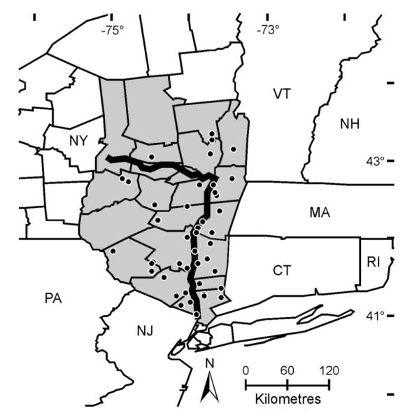
Map of the study area. The locations of tick density estimates are represented as black dots, the Hudson and Mohawk Rivers in a bold line, and the counties of New York State considered in this study are shaded.
Materials and Methods
Tick sampling
Nymphal and adult I. scapularis ticks were collected from a total of 44 sites across 22 counties in the Hudson River Valley, New York State (USA), from 2004 through 2010 (Fig. 1). Collection sites were chosen based on forested areas for which access was obtained. Not all collection sites were visited each year. Host-seeking ticks were collected by standardized dragging using a 1-m2 piece of white flannel or canvas (Ginsberg and Ewing 1989). Tick density estimates were calculated as the number of ticks collected by drag sampling divided by the total area surveyed (m2). Sampling locations were visited during June–August to estimate nymphal densities and during March–May and October–November to estimate adult tick densities. Density estimates of adults co-occurring during nymphal collection were included in the analyses. Adult ticks collected during the spring were considered the same cohort as those collected the previous fall in all analyses (see Tick phenology). Each sampling visit obtained a single density estimate for the appropriate tick stage. Tick collection efforts resulted in the collection of 7,140 nymphs (from 171 sampling visits) and 12,462 adults (from 238 sampling visits). Collection effort was evenly distributed across years except 2005 where only 20 density estimates were recorded.
Tick phenology
In northeastern North America, larval ticks hatch from egg masses and actively seek their first blood meal host, often a small mammal or bird, in late summer. After successfully feeding, larvae drop from hosts, molt to the nymphal stage, and overwinter in a quiescent state until they actively seek a second blood meal host, often a small mammal or bird, in early summer. Nymphal ticks that successfully feed drop from their host and molt to the adult stage which seeks a third host, often a white-tailed deer, in the fall. Adult females feed and mate on hosts and detach prior to producing eggs that hatch the following year. Adult females that fail to find a host in the fall overwinter and resume activities the following spring. The average life cycle of the blacklegged tick occurs over two years, with the overwhelming majority of time spent detached from hosts and directly subject to environmental elements and with little ability to move distances greater than 1 meter. The days spent on animal hosts—approximately three, five, and twelve for the larvae, nymphs, and adults, respectively—provide an opportunity for dispersal. More extensive descriptions of tick phenology are available in prior publications (e.g., Daniels et al. 1996, Ostfeld et al. 1996, Randolph 1998, Ogden et al. 2006, Ogden et al. 2008a).
Covariate selection
Tick density estimates may be affected by environmental conditions that modify questing behavior during sampling (e.g., Hubálek et al. 2003, Perret et al. 2003, Perret et al. 2004, Crooks and Randolph 2006, Devevey and Brisson 2012). To account for this source of error, environmental factors including temperature, humidity, wind conditions, and cloud cover were recorded at each sampling session. We included collection week to consider tick seasonal patterns (see Tick phenology). To assess factors that affect tick densities, we selected variables previously hypothesized to affect tick survival, rates of development, and/or habitat suitability. Mean annual temperature was utilized to consider tick development and survival rate (Lindsay et al. 1995, Brownstein et al. 2003, Ogden et al. 2004). Temperature and precipitations during the warmest quarter were included to consider desiccation risk during summer months (Bertrand and Wilson 1996, Brownstein et al. 2003). Precipitation during the coldest quarter was used to assess the potential effect of snow cover or excessive moist conditions at the soil level (Guerra et al. 2002). Temperature during the coldest quarter was incorporated to consider overwinter survival (Lindsay et al. 1995, Brownstein et al. 2003). Landcover indices were included to consider habitat quality (Lindsay et al. 1998, Guerra et al. 2002, Allan et al. 2003, Brownstein et al. 2005). Importantly, the geographic position (latitude and longitude) and collection year were included in all models to explain the variance over time and space that can be attributed to population growth (see also Spatial and temporal autocorrelation). The spatial and temporal variables are essential to capture the dynamic nature of the changing population.
Covariate data sources
Climatic data were extracted from Worldclim with 30-arcseconds resolution (Hijmans et al. 2005). Landscape data with 90 m resolution were obtained from the Land Cover Trends Project (Trends study year 2000; US Geological Survey, http://landcovertrends.usgs.gov/) to estimate the proportion of total landcover corresponding to forest, urban, and shrubs using a 7 × 7 pixels kernel. The total area of forest patches (minimum area 2 × 2 pixels) and ratio of forest perimeter to area were calculated using 50 m, 100 m, and 500 m search radii in Fragstats 3.3 (McGarigal et al. 2002). Landscape datasets were resampled to 30-arcseconds resolution to match the climate data resolution for spatial predictions using cubic interpolation. All datasets were windowed to match our study area (75°34′30″W, 73°W; 41°N, 45°N). Point values for sample locations were obtained by point to raster interception. GIS processing was performed using IDRISI Taiga (Clark Labs, Worcester, Massachusetts, USA) and ArcGis 9.3 (ESRI, Redlands, California, USA) with the Geospatial Modeling Environment 0.4.0 plug-in (Spatial Ecology LLC, http://www.spatialecology.com/gme).
Model development and validation
Multiple regression models were developed independently for each tick developmental-stage (nymph and adult). All models were developed using a subset of the data that included all estimates from 2004 through 2008, while the remaining years (2009–2010) were utilized only for model validation. Models were validated by linear regression of predicted to observed values (Rykiel 1996). We selected covariates, interactions between covariates (up to second order), and non-linear effects (up to second order) a priori to develop and evaluate competing models. Higher degree interactions and polynomial responses were not considered because of uncertainty in the biological interpretation. Akaike’s Information Criteria (Akaike 1974) corrected for small sample size (Burnham and Anderson 2002) (AICc) was employed to select the best performing models. Significant effects of covariates were evaluated using Bonferonni-corrected multiple regression analyses (Bland and Altman 1995, Abdi 2007).
Nymphal and adult tick density estimates from collections (individuals per m2) were extrapolated to individuals per 30-arcseconds square (~63 hectare) and ln transformed to achieve normally distributed data (for an extensive review of advantages and requirements of this approach see O’Hara and Kotze 2010). Four data points that had density estimates of zero could not be transformed and were removed from the analysis. Models that use count data (Poisson regressions and zero inflated Poisson regressions [Zeileis et al. 2007]) were explored to estimate biases introduced by the data transformation using the R package PSCL (R Development Core Team 2008). JMP 7.0 (SAS 2007) and SPSS 17 (SPSS 2008) were used for all remaining statistical analysis using Type IV sum of square.
Spatial and temporal autocorrelation
The geographic coordinates and year were included as covariates in all models to account for the spatial and temporal autocorrelation that is inherent in directional processes. Autocorrelation that is not accounted for by these covariates can reduce the effective degrees of freedom and can make the models prone to type I error. The residuals of the models were tested for autocorrelation using Moran’s I in Passage 2.0 (Rosenberg and Anderson 2011) and checked for departures from normality using the D’Agostino Omnibus test (D’Agostino and Pearson 1973, D’Agostino et al. 1990).
Human disease incidence as a function of tick densities
We used the models with higher explanatory power to estimate predicted mean nymph and adult density estimates per county and year by averaging the predicted densities within pixels included in each county. The county-wide mean densities were correlated with the human Lyme disease incidence (per 100,000 habitant), the most commonly-reported disease vectored by I. scapularis (Appendix: Tables A1 and A2). Two additional diseases that I. scapularis vectors—anaplasmosis and babesiosis—have a very low incidence and thus could not be correlated with tick densities. After initial data exploration, we used piecewise correlations to identify hinge values (or break points) a posteriori in the correlations between the predicted nymph and adult density estimates (McGee and Carleton 1970, Neter et al. 1996). The method identifies the parameters of two correlations, one above and one below an iteratively determined hinge value, by finding the threshold value that minimizes the sum of squares of the errors around each correlation. We verified that the piecewise correlations minimize the total sum of squares of errors compared with a single first or second degree polynomial correlation.
Results
Direct estimates of both nymphal and adult tick densities demonstrate that tick densities were greatest in lower latitudes of the study area and gradual decreased toward northern latitudes of the study area (Fig. 2A). The observed patterns in tick density estimates across space are similar to the observed patterns in reported human Lyme disease cases (Fig. 2B). Additionally, tick density estimates increased annually across the region with the exception of 2010. Examination of the dataset revealed that observed densities in 2010 were unusually low. For example, the average density of nymphs was 0.022 per m2 in 2010 in contrast with an average density of 0.036 nymphs per m2 detected in all the other years combined. Despite the pattern irregularity in 2010, the trend of increasing densities was apparent in the study region.
Fig. 2.
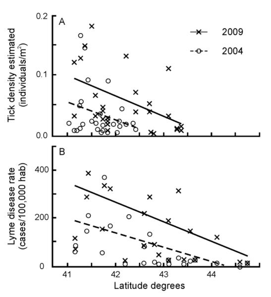
Illustrative representation of the temporal variation and spatial gradient of tick density estimates. (A) Nymphal tick densities were greater in later years and at lower latitudes of the study area, decreasing in northern latitudes. (B) The observed patterns in tick density estimates across space and time are similar to the observed patterns in reported human Lyme disease cases. 4 outliers (very high values; 1 from [A] and 3 from [B]) were removed from figures for graphical clarity but considered for trend lines.
The dynamic patterns in the tick density estimates observed in the raw data were captured in our models (Tables 1 and 2). The statistical models combining geographical, temporal, seasonal, environmental, climatic, and landscape covariates accounted for the majority of the variance in nymphal and adult tick density data (R2 = 0.64 and 0.62). Models omitting covariates from any of these categories accounted for substantially less of the variance in the observed density data (Table 1; see Appendix: Table A3). Variation in nymphal density estimates were best explained by a model that included geographic location, year, week of sampling (season), summer precipitation, minimum winter temperature, and proportion of forest cover (Table 1). Adult density estimates were best explained by a similar model that substituted winter precipitation for summer precipitation and included urbanization of the landscape (Table 1). Despite the simplicity of these models, each explained more than 60% of the variation in the observed tick densities. Several competing models for both nymphal and adult density had a similar fit to the observed data (ΔAICc < 2; see Appendix: Tables A3 and A4). These models differ from the best-fitting model only by alternative covariates that are highly-correlated with covariates in the best-fitting model. The coefficients estimated for each covariate, as well as the model predictions, are nearly identical among these best models indicating robustness to covariate selection. For example, replacing minimum winter temperature with annual mean temperature, covariates that are highly correlated (R2 = 0.71), in the best-fitting models for adult tick density estimates results in comparable coefficient estimates and similar fit to the data (R2 = 0.622 vs. R2 = 0.613, ΔAICc = 1.72). The models were insensitive to uneven stratified sampling effort by latitude (see Appendix: Table A5) and to effects of the log transformation of the response variable; models obtained with count data in Poisson regressions identified the same covariates as log-transformed models with equal probabilities, directions, and intensities (see Appendix: Table A6).
Table 1.
Illustrative list of tested models for nymph and adult density estimates ranked by ΔAICc. All models included year, week, latitude, and longitude. The models used in predictions are indicated with boldface.
| Regression models for density estimates | Parameters | ΔAICc | R 2 |
|---|---|---|---|
| Nymph model; additional covariates included | |||
| temporal and spatial covariates only | 6 | 9.3688 | 0.494 |
| summer prec, min winter temp | 8 | 6.1036 | 0.572 |
| summer prec, min winter temp, forest | 9 | 0 | 0.642 |
| summer prec, min winter temp, forestint, forest border/areaint | 11 | 1.7230 | 0.665 |
| Adult model; additional covariates included | |||
| temporal and spatial covariates only | 6 | 12.088 | 0.525 |
| winter prec, min winter temp | 8 | 12.263 | 0.510 |
| winter prec, min winter temp, forestint, urbanint | 11 | 0 | 0.622 |
| winter prec, min winter temp, forestint, forest2, urbanint | 12 | 1.0319 | 0.628 |
Notes: Abbreviations are: prec, precipitation; min, minimum; temp, temperature. Superscript int indicates interactions between variables. Superscript 2 indicates additional quadratic term. The forest border/area ratio indicated here was calculated with 100 m radius (see Methods: Covariate source).
Table 2.
Selected multiple regression models for nymph (R2 = 0.642, F = 26.151, df = 101, P < 0.0001) and adult (R2=0.622, F=29.036, df=159, P < 0.0001) densities. Statistics presented include the standard error term (SE), sum of square (SS), the F-statistic, and the probability value (P).
| Regression models for density estimates | Estimate | SE | SS | F | P |
|---|---|---|---|---|---|
| Parameters of nymph model | |||||
| Intercept | −328.2980 | 112.5677 | <0.0044 | ||
| Year | 0.3198 | 0.0575 | 19.1783 | 30.8890 | <0.0001 |
| Week | −0.1573 | 0.0197 | 39.6316 | 63.8317 | <0.0001 |
| Latitude | −4.2799 | 0.6687 | 25.4376 | 40.9704 | <0.0001 |
| Longitude | 1.5254 | 0.3261 | 13.5799 | 21.8722 | <0.0001 |
| Forest | −2.0926 | 0.4678 | 12.4262 | 20.0139 | <0.0001 |
| Min. winter temp | −0.0488 | 0.0189 | 12.0414 | 19.3941 | <0.0001 |
| Summer prec | −0.0832 | 0.0104 | 13.5668 | 21.8510 | <0.0001 |
| Parameters of adult model | |||||
| Intercept | −97.8929 | 136.7179 | 0.4750 | ||
| Year | 0.1993 | 0.0628 | 11.3173 | 10.0868 | 0.0018 |
| Week | 0.1183 | 0.0101 | 154.7724 | 137.9450 | <0.0001 |
| Latitude | −3.9760 | 0.9998 | 15.8149 | 15.8149 | 0.0001 |
| Longitude | 1.7186 | 0.4485 | 14.6829 | 14.6829 | 0.0002 |
| Forest | −1.8023 | 0.5519 | 10.6665 | 10.6665 | 0.0013 |
| Urban | 0.8306 | 0.4016 | 4.2773 | 4.27730 | 0.0402 |
| Forest × urban | −8.2613 | 1.8078 | 20.8835 | 20.8835 | <0.0001 |
| Min winter temp | −0.0588 | 0.0216 | 7.4265 | 7.42650 | 0.0071 |
| Winter prec | −0.0374 | 0.0111 | 11.3635 | 11.3635 | 0.0009 |
Notes: Abbreviations are: prec, precipitation; min, minimum; temp, temperature. Interaction is marked with × between variables.
All covariates included in the best-fitting models explaining nymphal density estimates are statistically significant in multiple regression analysis, and all but urbanization are significant in models explaining adult density estimates (Table 2). Interestingly, while both nymphal and adult tick densities increase annually, the year covariate is the predominant factor only for nymphal density estimates (explaining 30.79% of variance) and a significant although minor explanatory factor for adult density estimates (4.33%). Seasonal variation (week) accounts for the majority of variation in adult tick density estimates (59.17%) and a substantial fraction of the nymphal density estimates (19.76%). Geographic location explains 20% of observed variance in nymphal and 13% in adult density estimates. Precipitation and winter temperatures are correlated with tick density estimates (negatively and positively, respectively) and account for a small proportion of the variation in nymphal and adult tick density estimates (10% and 3%, respectively). Landscape covariates are also correlated with tick densities, explaining 10% and 15% of the variation in nymphal and adult density estimates, respectively.
The models that best explain nymphal density data from 2004 through 2008 successfully predicted the nymphal density estimates collected in 2009 and 2010 with 80% and 74% accuracy, respectively (Fig. 3A, B). The prediction for 2010 was consistently greater than the observed values although the general trend is maintained. The models developed with the 2004–2008 adult density estimate dataset had lower predictive power for 2009 adult density estimates (48%), primarily due to poor predictions for two locations (Fig. 3C). The model predictions for 2010 adult density estimates presented similar performance to those for nymphs (67% accuracy) and were similarly biased toward over-prediction (Fig. 3D).
Fig. 3.
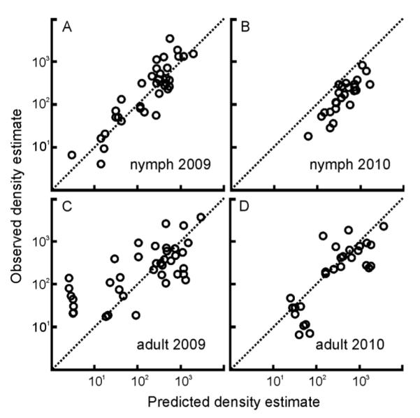
The nymph and adult density estimate regression models built using data from 2004–2008 accurately predict the tick density estimates in 2009 and 2010. Estimates predicted by the nymphal model explain (A) 80% of the variation in the observed nymph density estimates from 2009 (R2=0.8, n=35, P < 0.0001) and (B) 74% of the variation in the observed tick density estimates from 2010 (R2=0.74, n=26, P < 0.0001). Estimates predicted by the adult model explains (C) 48% of the variation in the observed adult density estimates from 2009 (R2 = 0.48, n = 40, P < 0.0001) and (D) 67% of the variation in the observed tick density estimates from 2010 (R2=0.67, n=29, P < 0.0001). Original units prior to log transformation are individuals/hectares. The dotted diagonal line through the origin represents the ideal correspondence (1:1) between observed and predicted density estimates.
The nymphal (Fig. 4A, B) and adult (Fig. 4C, D) density estimate models demonstrated good predictive power of trends over wide geographical areas with only the single bias in the 2010 dataset described above (Fig. 4D). The predicted surfaces of nymphal and adult tick density estimates differ in subtle details. For example, the nymphal density estimate model predicts a smooth surface with progressive transition between low and high predicted estimates (variance to mean ratio = 0.61 for 2009 and 0.59 for 2010 [Fig. 4B], suggesting a regular pattern). In contrast, the adult density estimate model predicts abrupt changes across the landscape (variance to mean ratio = 1.32 for 2009 and 1.28 for 2010 [Fig. 4D], suggesting a clustered pattern). The residuals from the linear models showed no departure from normality (D’Agostino omnibus test, α = 0.05) and no evidence of autocorrelation, indicating that the spatial and temporal autocorrelation inherent in the dataset was accounted for by the covariates in the models.
Fig. 4.

Spatial representation of predictions for nymph (2009 [A] and 2010 [B]) and adult (2009 [C] and 2010 [D]) density estimates. The performance of selected models are shown using the predicted collection values for the region plotted as a surface (original units prior to log transformation are individuals/30-arcsecond pixels) for year 2009 and 2010 and the observed collection values (circles). The observed values represent the average of multiple samples collected in the same year and location. Matching of color inside the circles with the continuous surfaces describes the accuracy of the model predictions.
Human Lyme disease incidence, the tick-borne disease with the greatest reported incidence in the region, was correlated with both nymphal and adult tick density estimates in a non-linear, threshold-type function (Fig. 5A, B). That is, human Lyme disease incidence remains at moderate levels at tick-collection densities below the optimal hinge values estimated using piecewise correlation analyses (hinge values equal 1.13 and 0.71 individuals per hectare for nymphs and adults respectively). When densities are greater than the hinge values, human Lyme disease incidence is linearly correlated with local tick density estimates and explains 45% and 42% (for nymphs and adults respectively) of the variation in human Lyme disease rates.
Fig. 5.

The relationship between model-predicted nymphal and adult density estimates (original units prior to log transformation are individuals/hectares) and the observed incidence of Lyme disease per county from 2004 to 2009. (A) Lyme disease incidence is significantly correlated with nymph density estimates greater than the hinge value (dotted line; hinge value=1.13 individuals hectare−1; R2=0.45, n=270, P < 0.0001) but not when estimates are lower than the hinge value (R2 = 0.02, n = 40, P > 0.05). (B) Similarly, the correlation between Lyme disease incidence and local adult densities is only significant for values greater that the hinge value (hinge value = 0.71 individuals hectare−1; R2 = 0.42, n = 281, P < 0.0001) but not when the estimates are lower than the hinge value (R2 = 0.02, n = 29, P > 0.05).
Discussion
In the northern hemisphere, the northern distribution and abundance of many organisms is limited by a complex combination of harsh environmental conditions and specific ecological characteristics. However, changes in one or several environmental factors can lead to dramatic increases in population densities. In this study, we used temporally- and spatially-structured data to characterize the population dynamics of the blacklegged tick, I. scapularis. Much of the heterogeneity in the density estimates of nymphal and adult ticks results from the annual population increases and to the marked latitudinal gradient (higher densities in southern areas and gradual decrease toward the north; Fig. 2A). The temporally- and spatially-structured data collected during dynamic changes in population size allowed confident identification of environmental and climatic factors that correlate with these changes. Including precise estimates of these factors into models accurately predicted tick density estimates in the near future (i.e., observed density estimates in the excluded datasets of 2009 and 2010). These models can allow the assessment of future risks of human contact with diseases commonly vectored by this tick species.
The density estimates of both tick life-stages were greatest in the southern regions and decreased with increasing latitudes (Fig. 2A). Further, tick density estimates appeared to increase annually at most locations across the region. These trends, which are apparent in the sampling data, were formalized and quantified in statistical models that incorporated time, space, and environmental factors as covariates to account for the dynamics in tick density estimates. Approximately half of the variation in tick density estimates of both life stages was accounted for by the covariates year, geographic location, and seasonality indicating large population dynamics on these temporal and spatial scales. The remaining explainable variation in tick density estimates could be attributed to environmental factors that were not correlated with the temporal or spatial factors.
The climatic and landscape covariates in our model account for a substantial proportion of the variation in tick density estimates in our dataset(Table 2). Our results support the hypothesis that habitat suitability and climate are important factors determining tick population growth rates and densities, as previously suggested (e.g., Guerra et al. 2002, Brownstein et al. 2005). This hypothesis is further supported by a previous study that classified the northeastern portion of our study area as unsuitable for I. scapularis populations prior to 1990 (Estrada-Peña 2002) suggesting that climate change and anthropogenic changes to the landscape altered habitat suitability, allowing I. scapularis to establish and increase. However, the underlying causes of the recent discovery of I. scapularis populations in the northern Hudson River Valley remain unclear. Although improvements in habitat suitability may have allowed previously-established populations to grow from very low densities to detectable levels, it is also possible that I. scapularis populations have only recently colonized the region. Future analyses of the migratory patterns of I. scapularis in the Hudson Valley will help to discriminate between these hypotheses and further clarify the effects of climate change and landscape variation on tick demography.
Environmental factors such as extreme winter temperatures, summer or winter precipitation, and landscape variables were correlated with densities estimates suggesting that these factors directly regulate tick population dynamics. This hypothesis is supported by experimental studies demonstrating that mean and extreme temperatures, precipitation, and landscape features can directly affect survival, development rate, or reproduction rate in I. scapularis ticks (e.g., Lindsay et al. 1995, Lindsay et al. 1998). However, these environmental factors are also likely to affect the populations of vertebrate species that are the primary food sources for ticks (Ostfeld et al. 2006, Brunner et al. 2011). The composition and densities of vertebrate species have an important role in regulating tick densities, suggesting that environmental factors may also act indirectly. Decoupling direct effects of environmental factors on tick population dynamics from indirect effects requires a comprehensive catalog of the distribution and abundance of each of the tens to hundreds of potential vertebrate hosts species (Anderson 1988) across the study area and throughout the collection duration. Unfortunately, the densities of few wildlife species have been estimated at local scales (Ostfeld et al. 2006) and none have been systematically estimated across the region of interest even at coarse-scales. The results of the current models can direct future work aimed at discriminating between the direct and indirect effects of the identified environmental factors.
The seasonal activity patterns of the tick life-stages dramatically affected the local density estimates for both the adult and nymphal ticks. The seasonality covariate accounted for this variation such that neither the estimates of annual increases in density across the region nor the estimates of the effects of the geographic location on population densities were affected by the sampling scheme. The effect of the seasonal activity pattern on immediate density estimates was expected as the seasonal activity patterns of the I. scapularis life-stages have been extensively documented (e.g., Daniels et al. 1996, Ostfeld et al. 1996, Randolph 1998, Ogden et al. 2006, Ogden et al. 2008a, Devevey and Brisson 2012). Variance in adult density estimates was strongly affected by the week of sample collection due to the two annual peaks of adult tick activity (Daniels et al. 1996). Surprisingly, excluding spring density estimates from the adult tick dataset results in a model that is nearly indistinguishable from that of the nymphs. In these models, less than 0.5% of the variation is accounted for by seasonality and other variables such as year (12.55%), geographical location (38.35%), and climatic covariates (32.1%) explain substantially more variance. Thus, our analyses suggest that the factors that affect the tick population densities are nearly identical regardless of the life-stage investigated, lending confidence to the robustness of these results.
The models that best described the data collected in 2004–2008 resulted in highly accurate predictions of tick densities estimates in 2009 and 2010 (Figs. 3 and 4). Thus, models that include broad-scale climatic and landscape variables are sufficient to predict the near-term densities of I. scapularis populations. Although all predictions were generally accurate, the model consistently predicted greater density estimates than were observed in the 2010 field-collection dataset suggesting that an important regional-scale factor in 2010 was not incorporated into the best fitting models produced from the 2004–2008 dataset. We expect that a climatic factor that showed little variation between 2004–2008, and thus was not included in the best models, fluctuated dramatically in 2010 resulting in the low tick density estimates observed. Despite the over-prediction in 2010, the spatial trend in the model predictions was consistent with the observed data suggesting that these models can have a direct public health translation. However, extrapolation of the model predictions to areas that are beyond the geographic range used to develop and calibrate the models should be regarded with caution. For example, the northwestern region of our prediction map is projected by both statistical models to have the lowest tick density estimates. Although these expectations are compatible with the general model of tick density estimates and anecdotal evidence of current tick densities, the use of specific numerical values obtained in this region should be discouraged. Further data with longer time series and wider geographical extent are needed to determine the long-term and coarse scale accuracy of these models.
The density estimates of blacklegged ticks explain a substantial proportion of the variation in the human risk of contracting diseases commonly vectored by I. scapularis (Fig. 5). Interestingly, these results suggest that the correlation between human incidence and tick densities is non-linear and disappears at low tick density estimates. Considering that the majority of the human cases of Lyme disease are attributable to transmission from the nymphal stage, the detected correlation with adult densities estimates should be considered as a proxy of general tick densities in the area. These data could suggest that there is a threshold population density of I. scapularis needed to support epidemiologically-relevant levels of B. burgdorferi in vector tick populations as previously suggested (Hamer et al. 2010). However, B. burgdorferi can be detected at low prevalence in animal hosts suggesting that low-level transmission may occur even at low I. scapularis densities (Oliver et al. 2006), potentially explaining the sporadic Lyme disease cases in areas with few I. scapularis ticks. This result reveals the importance of a non-trivial parameter that needs to be incorporated in the development of epidemiological models that aim to predict human risk based on vector densities. Incorporating microbial pathogen population dynamics along with vector densities in a spatial and temporal framework will likely increase the accuracy and predictive power of models that assess human disease risk.
Studies to accurately determine areas of high human disease risks are critical to developing effective vector control and disease mitigation strategies. Such assessments must consider the complex combination of environmental conditions and ecological requirements that affect the distribution and abundance of medically relevant organisms. In this study, we provide three explicit contributions: First, we show that statistical models including temporal, geographic, climatic, and land-use variables accurately determine tick density estimates. In this way, we promote the inclusion of these factors into models built to predict future tick densities which may be generalizable to other habitats. Second, we correlate the increases in tick density with human disease risk over time and space, demonstrating the direct public health relevance of such models. Third, we provide explicit maps that highlight high density estimates tick areas. These maps allow the general population to exercise additional preventive measures in high-risk areas and allow vector control agencies to target these areas for intervention. Effective vector control not only reduces disease risk within the targeted area, but can also slow the rate of progression of the tick into new regions.
Supplementary Material
Table A1. Rates of human Lyme disease cases per 100,000 habitants in Hudson River Valley counties (years 1994–2001).
Table A2. Rates of human Lyme disease cases per 100,000 habitants in Hudson River Valley counties (years 2002–2009).
Table A3. List of all competitive models identified for nymph density, ranked by ΔAICc. The selected model, used in prediction, is indicated with boldface. All models included year, week, latitude, and longitude.
Table A4. List of all competitive models identified for adult density, ranked by ΔAICc. The selected model, used in prediction, is indicated with boldface. All models included year, week, latitude, and longitude.
Table A5. In order to assess the robustness of our models to uneven sampling, we randomly selected subsets from each dataset to create datasets with locations evenly stratified by latitude. These subsets represent 60.9% and 41.42% of the dataset originally used for model development of nymphs and adults, respectively. The parameters estimates obtained with such unbiased subsets are remarkably similar to those obtained with the full dataset. The unbiased nymph model (Regression model for nymph density estimates using a randomly selected subset evenly stratified by latitude; R2 = 0.604, F = 12.874, df = 58, P <0.0001), with roughly 60% of the data points, is practically identical to the original (see Table 2). Two of the covariables (longitude and summer precipitations) are not significant after Bonferroni corrections when compared with the original model. The unbiased adult model (Regression model for adult density estimates using a randomly selected subset evenly stratified by latitude; R2 = 0.76, F = 21.151, df = 60, P < 0.0001), with roughly 40% of the data points, is similar to the original (see Table 2). Although exact parameters estimates and significance differ slightly, the relative effects and directions of each one are similar.
Table A6. Equivalent Poisson multiple regression models to the linear multiple regression selected for nymph (df = 101) and adult (df = 159) densities. Statistics presented include the standard error term (SE), Z-value, and the probability value (P).
Acknowledgments
C. E. Khatchikian and M. Prusinski contributed equally to this work. The authors would like to express their sincere gratitude to various NY State, county, local municipality, and private landowners for granting us use of their properties to conduct this research. We would also like to extend thanks to the following individuals for their assistance in collection and/or identification of ticks: J. Kokas, R. Falco, S. Kogut, J. H. Lee, M. VanDeusen, J. Hallisey, and a multitude of Entomological Assistants, student interns and county health department staff. Additional thanks to G. Lukacik for compiling human case numbers. We thank two reviewers for helpful comments on the manuscript. This work was supported by the Centers for Diseases Control and Prevention grant CK000170 and the National Institute of Health grants AI076342 and AI097137.
Literature Cited
- Abdi H. The Bonferroni and Sidak corrections for multiple comparisons. In: Salkind NJ, editor. Encyclopedia of measurement and statistics. Sage; Thousand Oaks, California, USA: 2007. pp. 103–107. [Google Scholar]
- Akaike H. A new look at the statistical model identification. IEEE Transactions on Automatic Control. 1974;19:716–723. [Google Scholar]
- Allan B, Keesing F, Ostfeld R. Effect of forest fragmentation on Lyme disease risk. Conservation Biology. 2003;17:267–272. [Google Scholar]
- Anderson JF. Mammalian and avian reservoirs for Borrelia burgdorferi. Annals of the New York Academy of Sciences. 1988;539:180–191. doi: 10.1111/j.1749-6632.1988.tb31852.x. [DOI] [PubMed] [Google Scholar]
- Bertrand MR, Wilson ML. Microclimate-dependent survival of unfed adult Ixodes scapularis (Acari:Ixodidae) in nature: life cycle and study design implications. Journal of Medical Entomology. 1996;33:619–627. doi: 10.1093/jmedent/33.4.619. [DOI] [PubMed] [Google Scholar]
- Bland JM, Altman DG. Multiple significance tests: the Bonferroni method. British Medical Journal. 1995;310:170. doi: 10.1136/bmj.310.6973.170. [DOI] [PMC free article] [PubMed] [Google Scholar]
- Brown JH, Stevens GC, Kaufman DM. The geographic range: size, shape, boundaries, and internal structure. Annual Review of Ecology and Systematics. 1996;27:597–623. [Google Scholar]
- Brownstein JS, Holford TR, Fish D. A climate-based model predicts the spatial distribution of the Lyme disease vector Ixodes scapularis in the United States. Environmental Health Perspectives. 2003;111:1152–1157. doi: 10.1289/ehp.6052. [DOI] [PMC free article] [PubMed] [Google Scholar]
- Brownstein JS, Skelly DK, Holford TR, Fish D. Forest fragmentation predicts local scale heterogeneity of Lyme disease risk. Oecologia. 2005;146:469–475. doi: 10.1007/s00442-005-0251-9. [DOI] [PubMed] [Google Scholar]
- Brunner JL, Cheney L, Keesing F, Killilea M, Logiudice K, Previtali A, Ostfeld RS. Molting success of Ixodes scapularis varies among individual blood meal hosts and species. Journal of Medical Entomology. 2011;48:860–866. doi: 10.1603/me10256. [DOI] [PubMed] [Google Scholar]
- Burnham KP, Anderson DR. Model selection and multimodel inference: a practical information-theoretic approach. Springer; New York, New York, USA: 2002. [Google Scholar]
- Connally NP, Ginsberg HS, Mather TN. Assessing peridomestic entomological factors as predictors for Lyme disease. Journal of Vector Ecology. 2006;31:364–370. doi: 10.3376/1081-1710(2006)31[364:apefap]2.0.co;2. [DOI] [PubMed] [Google Scholar]
- Crooks E, Randolph SE. Walking by Ixodes ricinus ticks: intrinsic and extrinsic factors determine the attraction of moisture or host odour. Journal of Experimental Biology. 2006;209:2138–2142. doi: 10.1242/jeb.02238. [DOI] [PubMed] [Google Scholar]
- D’Agostino R, Pearson ES. Tests for departure from normality. Empirical results for the distributions of b2 and √b1. Biometrika. 1973;60:613–622. [Google Scholar]
- D’Agostino RB, Belanger A, D’Agostino RB., Jr A suggestion for using powerful and informative tests of normality. The American Statistician. 1990;44:316–321. [Google Scholar]
- Daniels TJ, Boccia TM, Varde S, Marcus J, Le J, Bucher DJ, Falco RC, Schwartz I. Geographic risk for Lyme disease and human granulocytic ehrlichiosis in southern New York state. Applied and Environmental Microbiology. 1998;64:4663–4669. doi: 10.1128/aem.64.12.4663-4669.1998. [DOI] [PMC free article] [PubMed] [Google Scholar]
- Daniels TJ, Falco RC, Curran KL, Fish D. Timing of Ixodes scapularis (Acari: Ixodidae) oviposition and larval activity in southern New York. Journal of Medical Entomology. 1996;33:140–147. doi: 10.1093/jmedent/33.1.140. [DOI] [PubMed] [Google Scholar]
- Devevey G, Brisson D. The effect of spatial heterogenity on the aggregation of ticks on white-footed mice. Parasitology. 2012;139:915–925. doi: 10.1017/S003118201200008X. [DOI] [PMC free article] [PubMed] [Google Scholar]
- Diuk-Wasser MA, Vourc’h G, Cislo P, Hoen AG, Melton F, Hamer SA, Rowland M, Cortinas R, Hickling GJ, Tsao JI, Barbour AG, Kitron U, Piesman J, Fish D. Field and climate-based model for predicting the density of host-seeking nymphal Ixodes scapularis, an important vector of tick-borne disease agents in the eastern United States. Global Ecology and Biogeography. 2010;19:504–514. [Google Scholar]
- Estrada-Peña A. Increasing habitat suitability in the United States for the tick that transmits Lyme disease: a remote sensing approach. Environmental Health Perspectives. 2002;110:635–640. doi: 10.1289/ehp.110-1240908. [DOI] [PMC free article] [PubMed] [Google Scholar]
- Gage KL, Burkot TR, Eisen RJ, Hayes EB. Climate and vectorborne diseases. American Journal of Preventive Medicine. 2008;35:436–450. doi: 10.1016/j.amepre.2008.08.030. [DOI] [PubMed] [Google Scholar]
- Ginsberg HS, Ewing CP. Comparison of flagging, walking, trapping, and collecting from hosts as sampling methods for northern deer ticks, Ixodes dammini, and lone-star ticks, Amblyomma americanum (Acari: Ixodidae) Experimental and Applied Acarology. 1989;7:313–322. doi: 10.1007/BF01197925. [DOI] [PubMed] [Google Scholar]
- Guerra M, Walker E, Jones C, Paskewitz S, Cortinas MR, Stancil A, Beck L, Bobo M, Kitron U. Predicting the risk of Lyme disease: habitat suitability for Ixodes scapularis in the north central United States. Emerging Infectious Diseases. 2002;8:289–297. doi: 10.3201/eid0803.010166. [DOI] [PMC free article] [PubMed] [Google Scholar]
- Guisan A, Thuiller W. Predicting species distribution: offering more than simple habitat models. Ecology Letters. 2005;8:993–1009. doi: 10.1111/j.1461-0248.2005.00792.x. [DOI] [PubMed] [Google Scholar]
- Hamer SA, Tsao JI, Walker ED, Hickling GJ. Invasion of the Lyme disease vector Ixodes scapularis: implications for Borrelia burgdorferi endemicity. Ecohealth. 2010;7:47–63. doi: 10.1007/s10393-010-0287-0. [DOI] [PubMed] [Google Scholar]
- Härkönen L, Härkönen S, Kaitala A, Kaunisto S, Kortet R, Laaksonen S, Ylönen H. Predicting range expansion of an ectoparasite—the effect of spring and summer temperatures on deer ked Lipoptena cervi (Diptera: Hippoboscidae) performance along a latitudinal gradient. Ecography. 2010;33:906–912. [Google Scholar]
- Hijmans RJ, Cameron SE, Parra JL, Jones PG, Jarvis A. Very high resolution interpolated climate surfaces for global land areas. International Journal of Climatology. 2005;25:1965–1978. [Google Scholar]
- Hubálek Z, Halouzka J, Juøicová Z. Host-seeking activity of ixodid ticks in relation to weather variables. Journal of Vector Ecology. 2003;28:159–165. [PubMed] [Google Scholar]
- Jaenson TG, Jaenson DG, Eisen L, Petersson E, Lindgren E. Changes in the geographical distribution and abundance of the tick Ixodes ricinus during the past 30 years in Sweden. Parasites and Vectors. 2012;5:8. doi: 10.1186/1756-3305-5-8. [DOI] [PMC free article] [PubMed] [Google Scholar]
- Jaenson TGT, Lindgren E. The range of Ixodes ricinus and the risk of contracting Lyme borreliosis will increase northwards when the vegetation period becomes longer. Ticks and Tick-borne Diseases. 2011;2:44–49. doi: 10.1016/j.ttbdis.2010.10.006. [DOI] [PubMed] [Google Scholar]
- Jones KE, Patel NG, Levy MA, Storeygard A, Balk D, Gittleman JL, Daszak P. Global trends in emerging infectious diseases. Nature. 2008;451:990–993. doi: 10.1038/nature06536. [DOI] [PMC free article] [PubMed] [Google Scholar]
- Kaplan L, Kendell D, Robertson D, Livdahl T, Khatchikian C. Aedes aegypti and Aedes albopictus in Bermuda: extinction, invasion, invasion and extinction. Biological Invasions. 2010;12:3277–3288. [Google Scholar]
- Khatchikian C, Dennehy J, Vitek C, Livdahl T. Environmental effects on bet hedging in Aedes mosquito egg hatch. Evolutionary Ecology. 2010a;24:1159–1169. [Google Scholar]
- Khatchikian C, Sangermano F, Kendell D, Livdahl T. Evaluation of species distribution model algorithms for fine-scale container-breeding mosquito risk prediction. Medical and Veterinary Entomology. 2010b;25:268–275. doi: 10.1111/j.1365-2915.2010.00935.x. [DOI] [PMC free article] [PubMed] [Google Scholar]
- Krasnov BR, Poulin R, Shenbrot GI, Mouillot D, Khokhlova IS. Host specificity and geographic range in haematophagous ectoparasites. Oikos. 2005;108:449–456. [Google Scholar]
- Lindsay LR, Barker IK, Surgeoner GA, McEwen SA, Gillespie TJ, Addison EM. Survival and development of the different life stages of Ixodes scapularis (Acari: Ixodidae) held within four habitats on Long Point, Ontario, Canada. Journal of Medical Entomology. 1998;35:189–199. doi: 10.1093/jmedent/35.3.189. [DOI] [PubMed] [Google Scholar]
- Lindsay LR, Barker IK, Surgeoner GA, McEwen SA, Gillespie TJ, Robinson JT. Survival and development of Ixodes scapularis (Acari: Ixodidae) under various climatic conditions in Ontario, Canada. Journal of Medical Entomology. 1995;32:143–152. doi: 10.1093/jmedent/32.2.143. [DOI] [PubMed] [Google Scholar]
- Lounibos LP. Invasions by insect vectors of human disease. Annual Review of Entomology. 2002;47:233–266. doi: 10.1146/annurev.ento.47.091201.145206. [DOI] [PubMed] [Google Scholar]
- Materna J, Daniel M, Danielova V. Altitudinal distribution limit of the tick Ixodes ricinus shifted considerably towards higher altitudes in Central Europe: results of three years monitoring in the Krkonose Mts. (Czech Republic) Central European Journal of Public Health. 2005;13:24–28. [PubMed] [Google Scholar]
- McGarigal K, Cushman SA, Neel MC, Ene E. FRAGSTATS: spatial pattern analysis program for categorical maps. University of Massachusetts; Amherst, Massachusetts, USA: 2002. [Google Scholar]
- McGee VE, Carleton WT. Piecewise regression. Journal of the American Statistical Association. 1970;65:1109–1125. [Google Scholar]
- Neter J, Kutner MH, Nachtsheim CJ, Wasserman W. Applied linear regression models. Third edition Irwin; Chicago, Illinois, USA: 1996. [Google Scholar]
- O’Hara RB, Kotze DJ. Do not log-transform count data. Methods in Ecology and Evolution. 2010;1:118–122. [Google Scholar]
- Ogden NH, Bigras-Poulin M, Hanincova K, Maarouf A, O’Callaghan CJ, Kurtenbach K. Projected effects of climate change on tick phenology and fitness of pathogens transmitted by the North American tick Ixodes scapularis. Journal of Theoretical Biology. 2008a;254:621–632. doi: 10.1016/j.jtbi.2008.06.020. [DOI] [PubMed] [Google Scholar]
- Ogden NH, Lindsay LR, Beauchamp G, Charron D, Maarouf A, O’Callaghan CJ, Waltner-Toews D, Barker IK. Investigation of relationships between temperature and developmental rates of tick Ixodes scapularis (Acari: Ixodidae) in the laboratory and field. Journal of Medical Entomology. 2004;41:622–633. doi: 10.1603/0022-2585-41.4.622. [DOI] [PubMed] [Google Scholar]
- Ogden NH, Lindsay LR, Morshed M, Sockett PN, Artsob H. The emergence of Lyme disease in Canada. Canadian Medical Association Journal. 2009;180:1221–1224. doi: 10.1503/cmaj.080148. [DOI] [PMC free article] [PubMed] [Google Scholar]
- Ogden NH, Maarouf A, Barker IK, Bigras-Poulin M, Lindsay LR, Morshed MG, O’Callaghan CJ, Ramay F, Waltner-Toews D, Charron DF. Climate change and the potential for range expansion of the Lyme disease vector Ixodes scapularis in Canada. International Journal of Parasitology. 2006;36:63–70. doi: 10.1016/j.ijpara.2005.08.016. [DOI] [PubMed] [Google Scholar]
- Ogden NH, St-Onge L, Barker IK, Brazeau S, Bigras-Poulin M, Charron DF, Francis CM, Heagy A, Lindsay LR, Maarouf A, Michel P, Milord F, O’Callaghan CJ, Trudel L, Thompson RA. Risk maps for range expansion of the Lyme disease vector, Ixodes scapularis, in Canada now and with climate change. International Journal of Health Geography. 2008b;7:24. doi: 10.1186/1476-072X-7-24. [DOI] [PMC free article] [PubMed] [Google Scholar]
- Oliver J, Means RG, Kogut S, Prusinski M, Howard JJ, Layne LJ, Chu FK, Reddy A, Lee L, White DJ. Prevalence of Borrelia burgdorferi in small mammals in New York State. Journal of Medical Entomology. 2006;43:924–935. doi: 10.1603/0022-2585(2006)43[924:pobbis]2.0.co;2. [DOI] [PubMed] [Google Scholar]
- Ostfeld RS, Canham CD, Oggenfuss K, Winchcombe RJ, Keesing F. Climate, deer, rodents, and acorns as determinants of variation in Lyme-disease risk. PLoS Biology. 2006;4:e145. doi: 10.1371/journal.pbio.0040145. [DOI] [PMC free article] [PubMed] [Google Scholar]
- Ostfeld RS, Hazler KR, Cepeda OM. Temporal and spatial dynamics of Ixodes scapularis (Acari: Ixodidae) in a rural landscape. Journal of Medical Entomology. 1996;33:90–95. doi: 10.1093/jmedent/33.1.90. [DOI] [PubMed] [Google Scholar]
- Parkinson AJ, Berner J. Climate change and impacts on human health in the Arctic: an international workshop on emerging threats and the response of Arctic communities to climate change. International Journal of Circumpolar Health. 2009;68:84–91. doi: 10.3402/ijch.v68i1.18295. [DOI] [PubMed] [Google Scholar]
- Perret J-L, Guerin PM, Diehl PA, Vlimant M. l., Gern L. Darkness induces mobility, and saturation deficit limits questing duration, in the tick Ixodes ricinus. Journal of Experimental Biology. 2003;206:1809–1815. doi: 10.1242/jeb.00345. [DOI] [PubMed] [Google Scholar]
- Perret J-L, Rais O, Gern L. Influence of climate on the proportion of Ixodes ricinus nymphs and adults questing in a tick population. Journal of Medical Entomology. 2004;41:361–365. doi: 10.1603/0022-2585-41.3.361. [DOI] [PubMed] [Google Scholar]
- R Development Core Team . R: A language and environment for statistical computing. R Foundation for Statistical Computing; Vienna, Austria: 2008. [Google Scholar]
- Randolph SE. Ticks are not insects: consequences of contrasting vector biology for transmission potential. Parasitology Today. 1998;14:186–192. doi: 10.1016/s0169-4758(98)01224-1. [DOI] [PubMed] [Google Scholar]
- Rosenberg MS, Anderson CD. PASSaGE: pattern analysis, spatial statistics and geographic exegesis. Version 2. Methods in Ecology and Evolution. 2011;2:229–232. [Google Scholar]
- Rykiel EJ. Testing ecological models: the meaning of validation. Ecological Modelling. 1996;90:229–244. [Google Scholar]
- SAS . JMP. Version 7 SAS Institute; Cary, North Carolina, USA: 2007. [Google Scholar]
- SPSS . SSPS. Version 13 SPSS; Chicago, Illinois, USA: 2008. [Google Scholar]
- Sutherst R, Bourne A. Modelling nonequilibrium distributions of invasive species: a tale of two modelling paradigms. Biological Invasions. 2009;11:1231–1237. [Google Scholar]
- Taylor LH, Latham SM, Woolhouse ME. Risk factors for human disease emergence. Philosophical Transactions of the Royal Society B: Biological Sciences. 2001;356:983–989. doi: 10.1098/rstb.2001.0888. [DOI] [PMC free article] [PubMed] [Google Scholar]
- Zeileis A, Kleiber C, Jackman S. Regression models for count data in R. Department of Statistics and Mathematics, Vienna University of Economics and Business Administration; Vienna, Austria: 2007. (Research Report Series). [Google Scholar]
Associated Data
This section collects any data citations, data availability statements, or supplementary materials included in this article.
Supplementary Materials
Table A1. Rates of human Lyme disease cases per 100,000 habitants in Hudson River Valley counties (years 1994–2001).
Table A2. Rates of human Lyme disease cases per 100,000 habitants in Hudson River Valley counties (years 2002–2009).
Table A3. List of all competitive models identified for nymph density, ranked by ΔAICc. The selected model, used in prediction, is indicated with boldface. All models included year, week, latitude, and longitude.
Table A4. List of all competitive models identified for adult density, ranked by ΔAICc. The selected model, used in prediction, is indicated with boldface. All models included year, week, latitude, and longitude.
Table A5. In order to assess the robustness of our models to uneven sampling, we randomly selected subsets from each dataset to create datasets with locations evenly stratified by latitude. These subsets represent 60.9% and 41.42% of the dataset originally used for model development of nymphs and adults, respectively. The parameters estimates obtained with such unbiased subsets are remarkably similar to those obtained with the full dataset. The unbiased nymph model (Regression model for nymph density estimates using a randomly selected subset evenly stratified by latitude; R2 = 0.604, F = 12.874, df = 58, P <0.0001), with roughly 60% of the data points, is practically identical to the original (see Table 2). Two of the covariables (longitude and summer precipitations) are not significant after Bonferroni corrections when compared with the original model. The unbiased adult model (Regression model for adult density estimates using a randomly selected subset evenly stratified by latitude; R2 = 0.76, F = 21.151, df = 60, P < 0.0001), with roughly 40% of the data points, is similar to the original (see Table 2). Although exact parameters estimates and significance differ slightly, the relative effects and directions of each one are similar.
Table A6. Equivalent Poisson multiple regression models to the linear multiple regression selected for nymph (df = 101) and adult (df = 159) densities. Statistics presented include the standard error term (SE), Z-value, and the probability value (P).