Abstract
Background
Heterogeneity in the response to PM2.5 is hypothesized to be related to differences in particle composition across monitoring sites which reflect differences in source types as well as climatic and topographic conditions impacting different geographic locations. Identifying spatial patterns in particle composition is a multivariate problem that requires novel methodologies.
Objectives
Use cluster analysis methods to identify spatial patterns in PM2.5 composition. Verify that the resulting clusters are distinct and informative.
Methods
109 monitoring sites with 75% reported speciation data during the period 2003–2008 were selected. These sites were categorized based on their average PM2.5 composition over the study period using k-means cluster analysis. The obtained clusters were validated and characterized based on their physico-chemical characteristics, geographic locations, emissions profiles, population density and proximity to major emission sources.
Results
Overall 31 clusters were identified. These include 21 clusters with 2 or more sites which were further grouped into 4 main types using hierarchical clustering. The resulting groupings are chemically meaningful and represent broad differences in emissions. The remaining clusters, encompassing single sites, were characterized based on their particle composition and geographic location.
Conclusions
The framework presented here provides a novel tool which can be used to identify and further classify sites based on their PM2.5 composition. The solution presented is fairly robust and yielded groupings that were meaningful in the context of air-pollution research.
Keywords: Multi-pollutant mixtures, Cluster analysis, Effect modification, Air pollution profiles, k-Means
1. Introduction
First demonstrated by the Harvard Six-City study (Dockery et al., 1993) and the American Cancer Society Study (Pope et al., 1995), the association between PM and mortality has been replicated in many populations, both within the United States and abroad (Pope and Dockery, 2006). However, the magnitude of the effect has displayed considerable heterogeneity across studies (Bell et al., 2005; Janssen et al., 2002; Samet et al., 2000; Zanobetti et al., 2002). It is possible that this observed heterogeneity of effect may be attributed to the considerable differences in the PM composition across these study sites (Bell et al., 2007). This is further confirmed by investigations that attribute different levels of toxicity to particles from different sources (Laden et al., 2000; Mar et al., 2000; Zhou et al. (2011)). Toxicological studies have demonstrated the toxic potential of many individual PM components including sulfate, zinc, nickel and lead (Chuang et al., 2007; Gao et al., 2004; Lippmann et al., 2006; O’Neill et al., 2005).
The importance of considering multi-pollutant mixtures in air pollution was highlighted in 2004 by the National Academies of Science (NAS) (NRC, 2004). In response, the EPA is in the process to develop a multi-pollutant air quality management plan as described in their Multi-Pollutant Report of 2008 (EPA, 2008). Adopting a multi-pollutant approach is extremely challenging due to the highly complex interactions between source emissions, atmospheric processes and effects on human health and ecosystems. One of the key components of a multi-pollutant approach is the ability to capture the multivariate relationship between pollutants at a given site. A better grasp of this relationship will enhance our understanding of the interaction between pollutants as well as further the human health effects related to exposure to these complex mixtures.
The EPA has considered a variety of ways in which air pollutants might interact with each other (Table 1). Practically however, because of a knowledge gap in the field, the EPA is forced to consider all pollutant interactions as additive (Mauderly et al., 2010). Populations are exposed daily to complex mixtures of pollutants, some of which are known or suspected to cause health effects at ambient concentrations. Understanding the effect of the mixtures on health, rather than the effect of the individual components is a crucial step that must be undertaken in order to further our knowledge of this field. Therefore, it is essential that exposure assessment develop new tools to describe population exposures that moves beyond relating individual pollutant concentration at a given site on a given day.
Table 1.
Interaction of pollutants.
| (EPA, 2000) | |
|---|---|
| Additivity: | Effect of the combination equals the sum of individual effects |
| Synergism: | Effect of the combination is greater than the sum of individual effects |
| Antagonism: | Effect of the combination is less than the sum of individual effects |
| Inhibition: | A component having no effect reduces the effect of another component |
| Potentiation: | A component having on effect increases the effect of another component |
| Masking: | Two components have opposite, canceling effects such that no effect is observed from the combination |
There are currently a limited number of approaches that allow for the investigation of multi-pollutant mixtures in epidemiological studies (Dominici et al., 2010; Vedal and Kaufman, 2011). Exposure data is typically represented in high dimensionality data sets in which each pollutant is assigned a concentration for each time period of observation. Previous published multivariate approaches have included factor analysis methods and principle component methods such as specific rotation factor analysis (Koutrakis and Spengler, 1987), absolute principal-component analysis (Thurston and Spengler, 1985), UNMIX (Henry and Kim, 1990; Kim and Henry, 1999) and positive matrix factorization (Paatero and Tapper, 1994). These methods have been successful at identifying individual source contributions to integrated daily measurements samples at a specific or given site. The results of these multivariate methods are used by epidemiologists in time series analysis to investigate the health effects associated with specific sources (Schwartz et al., 2002; Thurston et al., 2005).
We propose an approach that uses cluster analysis to identify spatial patterns in air pollution data. Short- and long-term patterns in air pollution as well as spatial distribution patterns have been identified and described in the literature (Beelen et al., 2009; Jerrett et al., 2005; Koutrakis et al., 2005; Lefohn et al., 2010). At a single site, these patterns are the result of diurnal variations in UV intensity, season, temperature, cloud cover, mixing height as well as changes in source emissions such as higher traffic density on weekdays, increased power plant emissions during high demand periods and increase wood combustion in the winter. Between sites, differences in air pollution patterns can be attributed to different source types, different climatic conditions, distribution of regional pollutants over a geographic area and differences in soil composition.
Unsupervised cluster analysis encompasses a broad range of algorithms that identify multivariate patterns in data sets. Two broad categories of these algorithms are hierarchical and partitioning algorithms. The output of the algorithm may be “hard” if each observation is attributed to only one cluster or “fuzzy” if an observation may be assigned to a certain degree to more than one cluster. In this analysis, we were interesting in identifying a “hard” solution so that each site was uniquely assigned to a single cluster.
Recently, we used cluster analysis to identify distinct daily multi-pollutant profiles at a given site, Boston, MA, (Austin et al., 2012). Clustering has been used previously to describe diurnal variation in gaseous and particle pollutants (Adame et al., 2012; Flemming et al., 2005). K-means clustering was used by Kim et al. (2008) in order to group sites based on the temporal fluctuation of PM2.5. Hierarchical clustering has also been used to identify distinct sources of volatile organic compounds based on the grouping of the measured concentrations (Kavouras et al., 2001). It has also been used to provide a description of regional chemical and transport processes associated with particular regimes and can inform which sources may be most important in the development of pollution episodes. Beaver and Palazoglu (2006) used an aggregated solution of k-means cluster analysis to characterize classes of ozone episodes occurring in the San Francisco bay. Pakalapati et al. (2009) used hierarchical clustering and sequencing to group air flow patterns associated with elevated ozone concentrations. Cluster analysis has also been used to cluster back trajectories to identify different classes of synoptic regimes over the duration of the trajectories (Comrie, 1996; Taubman et al., 2006).
In this paper, cluster analysis will be used to group sites across the United States based on their PM2.5 composition profiles using data collected between 2003 and 2008. The main interest is identifying long-term differences in the composition of PM2.5 across the different sites. These clusters of cities will then be characterized and validated based on physico-chemical characteristics, geographic locations, emission profiles, population density and position with respect to major emitter sources. It is anticipated that this novel approach will allow for a better understanding of the heterogeneity in PM2.5 composition across the United States. We hope that the identified clusters can be used to further investigate the heterogeneity in the relation-ship between PM2.5 concentration and mortality and morbidity across the United States.
2. Methods
2.1. Data collection
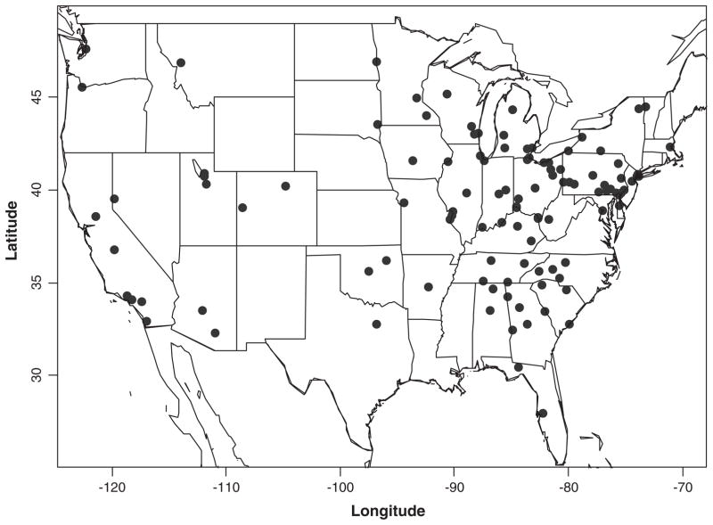
Data for this analysis was obtained from the HEI Air Quality Database (2010). This database includes pollutant concentrations from the EPA’s AQS Particulate Matter Air Quality Data. The PM2.5 mass and speciation data is available for 54 CORE sites and 234 supplemental sites from 2000 to 2010. These are 24-h samplers, midnight to midnight local standard time, with different sampling frequencies depending on the site location. Emissions data for each site is obtained from the National Emissions Inventory Data of 2002 and Census population data from the 2000 Census. We require that sites have less than 25% missing observations for the elements of interest. In addition, we require that each season within the time period has less than 25% missing data. This is to ensure that the site means are not unduly influenced by missing data within a given season. This resulted in 109 sites with complete data sets between January 2003 and December 2008. These dates were chosen in order to maximize the number of sites with 5 years of complete data. At each site, sampling occurred every 3rd or every 6th day throughout the year. Fig. 1 presents the location of the sampling sites.
Fig. 1.
Chemical speciation sites (n = 109).
2.2. Data preparation
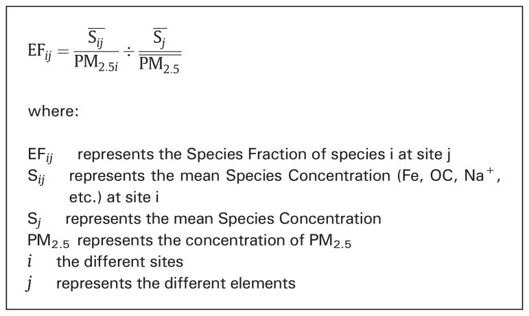
The variables used in the clustering were the following components of PM2.5: total EC, total OC, , Na+, , Se, Si, Ca, Fe, Ni, V, Cu, Zn, Pb, Mn, As, Cr, and K. Other elements obtained as part of the speciation of the filters were considered were excluded either because of the analytical measurement was judged to be unreliable or because a large proportion of the measurements were below the detection limit. For each site, an overall site mean of each variable was obtained. These means were divided by the mean PM2.5 concentration of that site to create a unique set of species fractions used to characterize the PM2.5 composition. These species fractions reflect the unique interplay of sources and meteorology at each site and they describe the composition of PM2.5 in a given element at that site (Eq. 1). To eliminate differences in the order of magnitude between concentration levels of the measured pollutants, the species fractions were transformed to a robust z-score as described in Eq. 2.
Eq. 1.
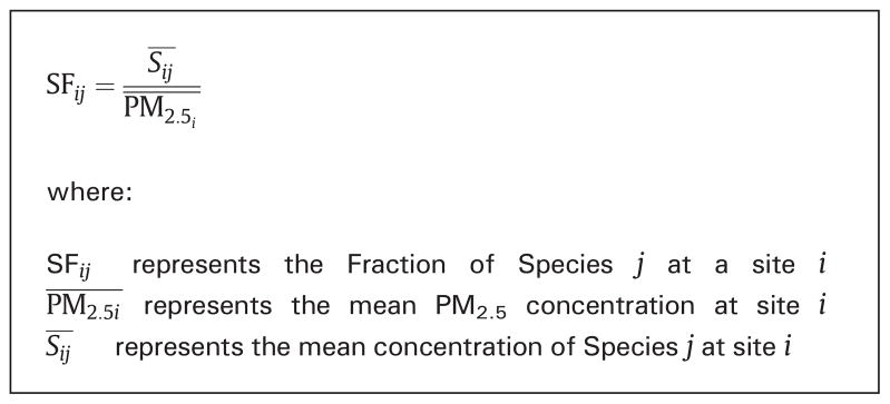
Species fraction.
Eq. 2.
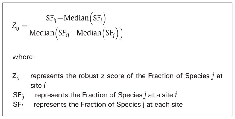
Modified Z-score.
2.3. Clustering
The main objective of this analysis was to cluster together cities with the most similar species fractions. Clustering of the mean values of the multi-pollutant profiles represents the overall population exposures in these cities over the study period. These clusters may improve our understanding of the heterogeneity in the long-term effects of PM2.5 exposure among populations.
The k-means algorithm used was developed by Hartigan and Wong (1979). It seeks to partition M points in N dimensions into k clusters. This iterative algorithm searches for a local solution that minimizes the Euclidean distance between the observations and the cluster centers. Advantages of the k-means algorithm are that it is easily implemented and has been used in a wide range of applications and is computationally efficient (Jain et al., 1999; Steinley, 2006). It has also been suggested that this algorithm is somewhat less sensitive to outliers than hierarchical clustering methods (Punj and Stewart, 1983). The initial k-values used in the algorithm can be randomly selected from the dataset being clustered, or the initial values can be specified by the user. In this case, we chose to specify the initial values of the clusters in order to increase the stability of the solution. Several methods have been proposed to initialize k-means. We used hierarchical clustering (described below) to identify k-centers and then using these centers to initialize k-means. Maitra et al. (2010) found this method of initializing k-means performed best for small datasets. Following the hierarchical analysis with k-means had the advantage of minimizing the impact of outlier points on the solution.
A major obstacle in using k-means is that the number of clusters (k) must be assigned a priori based either on pre-existing knowledge of the data or observable characteristics of the data set. Although there was no pre-existing knowledge of the number of unique spatial clusters to expect, we used characteristics of air pollutant mixtures in order to make the best possible selection. This is consistent with the recommendation of Jain et al. (1999) that subject specific knowledge is the best way to select the number of clusters. We considered the variability of pre-defined pollutant ratios within each cluster. Solutions with less total variability within the clusters were judged to be better than solutions with more variability within each cluster. Pollutant concentration ratios considered were: , EC/OC, Ni/V and Fe/Si. The rational was that solutions that were better at recognizing sites with similar pollution profiles would also minimize the variability of these important pollutant rations within each cluster. The variability of the ratios was reduced by maximizing the decrease in overall change in deviation as described in Eq. 3. The percent change in overall deviation represents how effectively different solutions capture the unique sources that contributed to the mixture at the individual sites. The advantage of using this indicator is that it explicitly uses knowledge of air pollution sources and contributions to inform the decision of how many clusters best describe the data. The rational for selecting these ratios is discussed below.
Eq. 3.
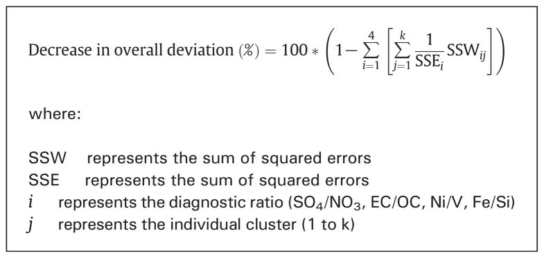
Change in overall deviation.
In addition to maximizing the decrease in the overall deviation, we sought to minimize the number of clusters containing a single site in each solution. As the total number clusters increases, the number of clusters including only 1 site likewise increases. This leads to a decrease in the % change in overall deviation without necessarily resulting in a more interpretable solution. K-means was performed using the function kmeans in R v.2.15.1.
2.4. Hierarchical clustering (Ward’s method)
Ward’s hierarchical clustering method (Ward, 1963) is an agglomerative process that begins with 1 cluster for every observation and then iteratively combines the points that lead to the minimal increase in the sum of squares. Because this method is agglomerative, the solution reached is constrained by the previous choices made by the algorithm. Therefore, for a given number of clusters, the solution reached by the Ward method is often not the solution that has the minimal sum of squares error. An advantage of this method is that it produces clusters that are relatively compact. It is criticized for sometimes producing clusters that are too small for the given data (Cormack, 1971). In this paper, hierarchical clustering was used to initialize k-means. It was also used after the analysis was completed to group together the clusters with the most similar enrichment factors. Hierarchical clustering was performed using the function hclust in R v2.15.1.
2.5. Enrichment factors
Enrichment factors were calculated in order to better compare the clusters. These enrichment factors represent the enrichment of a given constituent (element) of PM2.5 within a cluster as compared to the entire sample (Eq. 1).
2.6. Grouping clusters
Clusters were grouped together based on the enrichment factors within each cluster. The clustering was performed with hierarchical clustering using the hclust function in R v.2.15.1.
2.7. Comparing clustering solutions (Rand Index)
The Rand Index is a measure of similarity between two different partitions of the same data set. The Rand index ranges between 0 and 1 where 0 indicates that two data clusters do not agree on any pair of points and 1 indicating that the data clusters are exactly the same. The Rand Index represents a weight of the sites classified together in the two solutions versus the sites classified separately (Rand, 1971). In this paper, we used the adjusted Rand Index in order to compare different clustering solutions. The adjusted Rand Index, first proposed by Hubert and Arabie (1985) the adjusted Rand Index corrects the Rand Index for the random chance that pairs are classified together. Steinley (2004) suggested that an adjusted Rand Index greater than 0.9 reflected excellent agreement, values greater than 0.8 reflected good agreement, values greater than 0.65 indicated moderate agreement and less than 0.65 indicated poor agreement.
3. Results
3.1. Selecting the number of clusters k
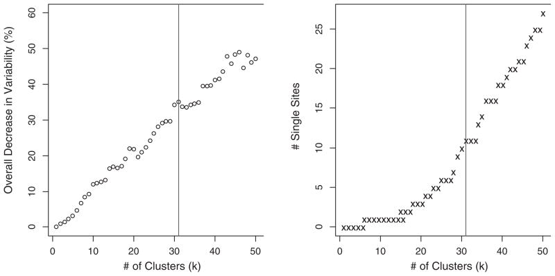
Selecting the value of k is a balance between the advantage in decreasing the variability in the diagnostic ratios within clusters and minimizing the number of single city clusters in a given solution. Fig. 2 presents the overall variability of the pollutant ratios alongside the number of single city clusters for solutions containing between 1 and 50 clusters. Based on the desire to balance these two features, 31 clusters was selected as the optimal value as it represents a significant drop in the overall decrease in variability measure (55% as compared to the dataset as a whole) while there are 11 clusters that contain only a single site. Other possible values of k were explored including k = 26 and k = 37. The solution of k = 26 was judged to not be satisfactory because it lacked good distinction between east and west coast cities. The solution for k = 37 was judged to be too unwieldy because of the high number of single city clusters.
Fig. 2.
Selecting the number of clusters (k).
3.2. Chemical characteristics
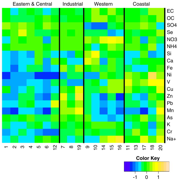
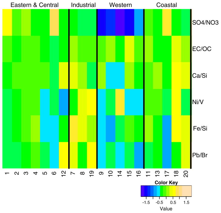
The chemical characteristics for the clusters containing 2 or more cities are presented as heatmaps in Fig. 4. These heatmaps represent the log of the enrichment factors of the pollutants of interest. For the heatmap representation, the enrichment factors were logarithmically transformed so that a value of 0 represents no enrichment, 1 represents 2.7 times enrichment and −1 represents 0.4 times enrichment. The clusters are presented in 4 groupings, where there are some overall similarities between the clusters in the same grouping. The similarities were determined based on hierarchical clustering of the enrichment factors in each cluster.
Fig. 4.
Heatmap of the log of the species enrichment factors by cluster.
3.3. Geographic distribution
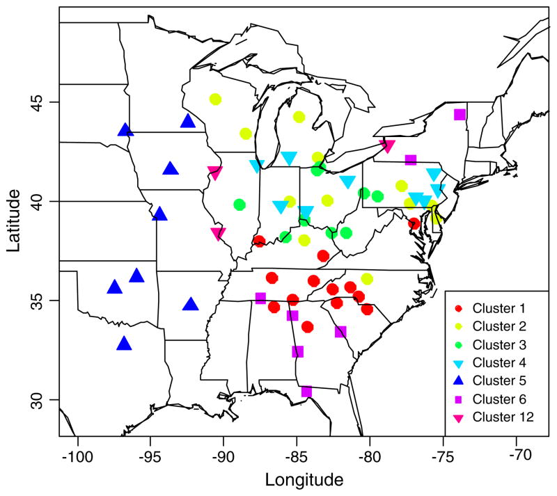
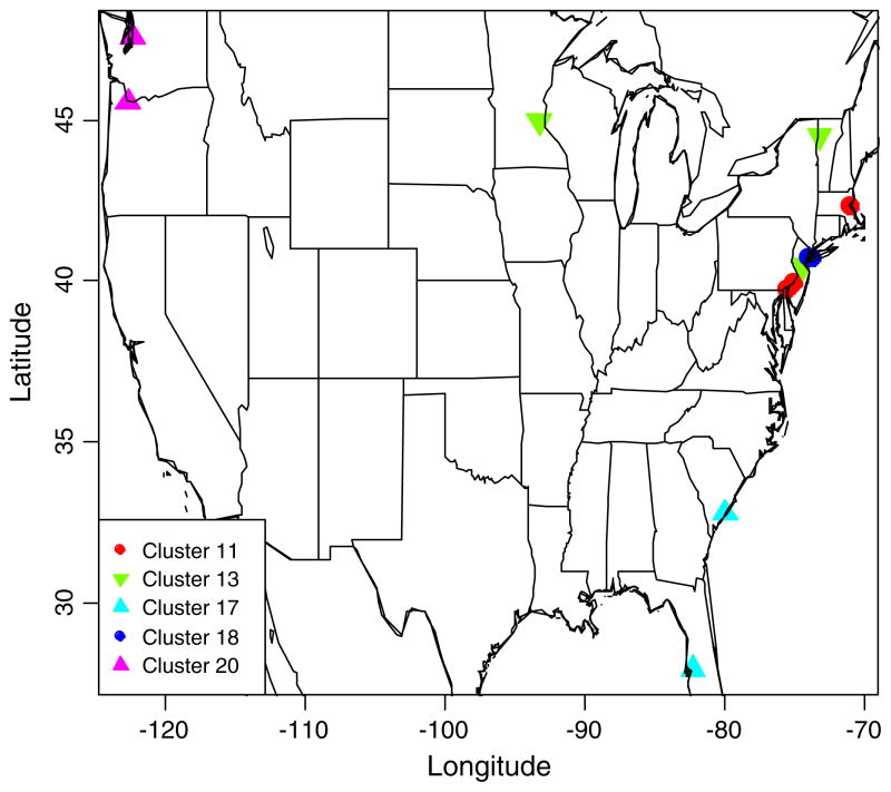
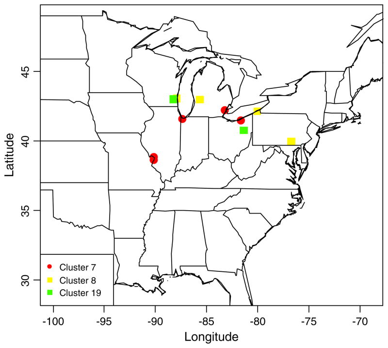
The locations of the 31 clusters identified are presented by group in Figs. 6–9. Evident in these maps, is that in some cases, sites that are geographically close belong to different clusters This is due to differences in composition, even at nearby monitoring sites and will be discussed further below. There is a clear separation between coastal and interior monitoring sites as well as between western, central and eastern sites. This agrees with previous studies showing that PM2.5 composition is related to geographic location and reflects the impacting sources and climatic conditions (Bell et al., 2007; Zanobetti and Schwartz, 2008).
Fig. 6.
Group 1, Eastern and Central clusters.
Fig. 9.
Group 4, Coastal clusters.
3.4. Concentration ratios
To aid in cluster interpretation, the log of the pollutant concentration ratios of selected species are presented as a heatmap in Fig. 5. Similar to the enrichment factors, the pollutant ratios have been normalized and represent the ratio in a particular cluster as compared to the entire sample. These normalized values have been log transformed so that a value of 0 represents no difference between the cluster and the sample as a whole, a value of 1 represents 2.7 times increase of the ratio within this cluster and sample as a whole and a value of −1 represents a 0.4 relationship between the ratio in this cluster and the whole sample.
Fig. 5.
Species ratios by cluster.
These ratios served as diagnostic tools to aid in attributing the sites to certain types of pollution regimes. Specifically: 1) higher ratios indicate a sulfate-dominated system, reflecting pre-dominance of power plant emissions vs. traffic; 2) higher EC/OC ratios suggest the predominance of primary carbon from traffic as opposed to secondary carbon. In some cases, lower EC/OC ratios can also be indicative of biogenic sources of air pollution; 3) the Ca/Si ratio is indicative of differences in soil composition between sites; 4) Ni and V are mostly released from oil combustion and the Ni/V ratio is affected by the temperature of the combustion process (Peltier and Lippmann, 2009). The ratio decreases as the temperature of combustion increases, leading to lower ratios in port locations exposed to emissions from maritime vessels as compared to those from oil-fired furnaces (assuming no impact of Ni or V of point sources, such as smelters); 5) higher Fe/Si ratios indicate a larger road dust contribution, relative to soil dust (assuming no impact of Fe point sources, such as steel mills); and 6) higher Pb/Br concentrations suggest enrichment of Pb with respect to background soil concentrations which can be observed near smelters. The ratios selected are by no means exhaustive and others may be of interest in other studies. These were thought to reflect the source profiles previously identified within the continental United States.
3.5. Site characteristics
Table 2 shows the classification within each cluster of sites deemed to be ‘urban’, ‘suburban’ and ‘rural’ based on the designations assigned by the EPA. Sites do not necessarily have the same designation within a cluster. In part, this may be related to whether classification was influenced by regional pollution versus local pollution.
Table 2.
Location type by cluster.
| Eastern US | Midwest | Central and Western | Coastal | |||||||||||||||||
|---|---|---|---|---|---|---|---|---|---|---|---|---|---|---|---|---|---|---|---|---|
| Cluster | 1 | 2 | 3 | 4 | 5 | 6 | 12 | 7 | 8 | 19 | 9 | 10 | 14 | 15 | 16 | 11 | 13 | 17 | 18 | 20 |
| # Sites | 13 | 12 | 10 | 9 | 8 | 7 | 3 | 5 | 4 | 2 | 4 | 3 | 2 | 2 | 2 | 3 | 3 | 2 | 2 | 2 |
| Rural | 1 | 7 | 3 | 1 | 1 | 3 | 0 | 0 | 0 | 0 | 0 | 1 | 0 | 0 | 0 | 0 | 1 | 0 | 0 | 0 |
| Suburban | 6 | 3 | 6 | 6 | 2 | 4 | 1 | 2 | 2 | 0 | 4 | 1 | 2 | 1 | 1 | 0 | 0 | 0 | 1 | 0 |
| Urban And Center City | 6 | 2 | 1 | 2 | 5 | 0 | 2 | 3 | 2 | 2 | 0 | 1 | 0 | 1 | 1 | 3 | 2 | 2 | 1 | 2 |
3.6. Sampling frequency
As discussed above sites were sampled either every three or six days. We wanted to verify that taking the global mean of these different sites did not lead to bias. In order to do so, we took the sites sampled every 3 days and calculated the global means based on every 6th sample day (dropping half the data). Of the 109 sites included in the study, 40 sites were sampled every 3rd day. We found that the ratios of the 6th day to 3rd day global mean are on average 1.00 with small standard deviations. Chromium showed a slightly higher standard deviation than other elements, but it was considered acceptable. Results are presented in Table 4.
Table 4.
Comparing 3 and 6 day averaging of elements.
| Element | Mean | SD | |
|---|---|---|---|
| PM2.5 | 1.00 | 0.03 | |
| EC | 1.00 | 0.03 | |
| OC | 1.00 | 0.02 | |
|
|
1.00 | 0.03 | |
| Se | 1.00 | 0.06 | |
| NO3 | 1.00 | 0.04 | |
|
|
1.00 | 0.04 | |
| Si | 1.00 | 0.04 | |
| Ca | 1.00 | 0.04 | |
| Fe | 1.00 | 0.03 | |
| Ni | 1.00 | 0.09 | |
| V | 1.02 | 0.05 | |
| Cu | 1.00 | 0.08 | |
| Zn | 1.00 | 0.04 | |
| Pb | 1.00 | 0.06 | |
| Mn | 1.00 | 0.04 | |
| As | 1.02 | 0.05 | |
| K | 1.01 | 0.08 | |
| Cr | 0.99 | 0.12 | |
| Na+ | 1.00 | 0.04 |
4. Discussion
Clustering data from 109 monitoring sites across the US yielded a solution with 31 distinguishable clusters. For each site, a single species fraction was obtained for the different PM2.5 components of interest. Although this approach does not account for season differences within sites, it captures the differences in long-term exposure across different cities in the United States. The 31 cluster solution was selected in order to minimize the number of clusters with only a single city as well as to minimize the variability of selected species ratios within each cluster. The overall PM2.5 composition differed substantially among clusters, indicating that this method does allow for an efficient classification of sites based on their differences in multi-pollutant relationships. To better understand the clustering results, clusters containing 2 or more cities were grouped into 4 main types based on the cluster PM2.5 enrichment by cluster. Although there are differences between the clusters in each of groups, overall they show similarities in chemical composition.
The clusters in the first grouping, Eastern US locations, show high to average ratios, suggesting the considerable impact of power plant emissions in these locations. This is consistent with previous studies that identify transported power plant emissions as a major source of regional air pollution in the Eastern United States (Bell et al., 2007). The clusters in the second grouping, are impacted by industrial processes and tend to be are located near large Iron and Steel Mills (EPA, 2011). These sites show high to average Ni/V, Fe/Si and Pb/Br ratios. The PM2.5 at these sites is also enriched in metals indicating the impact of industrial processes relative to the other US areas. This is consistent with research that shows significant contribution of heavy metals to the PM2.5 composition from industrial point sources (de Foy et al., 2012; Lee and Hopke, 2006). The third grouping, located in the Central and Western US, show significantly lower ratios which confirms that these sites are less impacted by power plant sources. The fourth grouping, located in coastal sites, has sites that have average to higher EC/OC ratios as well as higher Ni/V ratios. This is consistent with studies that have shown ship emissions to include high concentrations of Ni and V as well as high concentrations of EC and SO2 (Agrawal et al., 2008; Ault et al., 2010; Isakson et al., 2001).
4.1. Cluster description
4.1.1. Group 1 — Eastern and central US
There are 7 clusters in this group that include a total of 62 single sites. Some major characteristics of this group are the higher enrichment in , Se and average to low enrichment in elements such as Si, Ca, Fe, Ni, V, Zn and Mn. Cluster 1 shows particularly high ratios and lower Ni/V, Fe/Si and Pb/Br. Geographically, the sites in cluster 1 show geographical cohesiveness and are primarily in the Southeastern US. The sites in cluster 2 do not show as clear of a geographical connection; however, they are all predominantly located in rural and suburban locations. As can be expected, given their lower urbanization, these sites are less impacted by road emissions as indicated by a lower EC enrichment factor. Cluster 6 is similar to cluster 2 in that the sites are mostly in rural and suburban locations and the EC enrichment is low. A major difference is that cluster 6 also shows a significantly lower proportion. This suggests that these sites are less impacted by agricultural sources. The sites in cluster 3 are primarily located in the Midwest states. The PM2.5 in this cluster is heavily enriched by Se, an element whose major source is power plant emissions. Cluster 4 is similar to cluster 3 in both geographic location and chemical composition. However, this cluster shows less evidence of power plant contributions as evidenced by average enrichment factors for Se and . Cluster 5 has lower Ni/V and Fe/Si ratios. Unlike cluster 1 it also has a low Cu enrichment factor. This cluster is primarily located in the central part of the country and may represent locations that are affected by SOx emissions from power plants while having lower metal enrichment factors. Cluster 12 is distinct because of its relatively high Pb enrichment factor. Although the concentrations of Pb at these three locations (Davenport IA, Arnold MO and Buffalo NY) are within EPA guidelines, historic presence of Pb smelters in these locations may explain the apparent enrichment in this element. Although this cluster demonstrates high concentrations of Pb, it does not group with the clusters in group 2 because other metals do not show high enrichment factors.
4.1.2. Group 2 — Industrial sites
There are 3 clusters in this group that include a total of 11 sites. Geographically, many of these sites are located in the Midwest, more specifically in the Great Lakes region. The sites in this group are primarily urban, there are some suburban sites and no rural sites. The enrichment factors for Mn, Zn and Pb are particularly high. The ratios of Ni/V, Fe/Si and Pb/Br are all elevated in these locations as well. Cluster 7 has particularly high enrichment factors for Fe, Zn, Pb and Mn, while the enrichment in Ni is below average. Enrichment in these metals suggests contributions from industrial processes and smelters. Cluster 8 has average enrichment factors for Pb and Zn, although still shows a higher enrichment factor for Mn. Cluster 19 is enriched in Mn, suggesting possible anthropogenic sources in these locations such as alloy production and steel foundries. In fact, both Canton OH and Waukesha OH are the location of working steel foundries. Otherwise, cluster 19 is similar to cluster 7 except that the enrichment factor for Ni is higher in Cluster 19, while the enrichment factor for V is lower.
4.1.3. Group 3 — Central & Western US
There are 5 clusters in this group that include a total of 13 sites. The main commonality between these sites is the lower enrichment factor for sulfate and higher enrichment factor for. This results in low ratios across this group. Clusters 14, 15 and 16 are all located in California. Cluster 15 (Los Angeles area) has higher EC enrichment and the highest enrichment in . Cluster 14 is enriched in but unlike the other California clusters, it is very low in which suggests that there are fewer oil combustion sources impacting these sites.
4.1.4. Group 4 — Coastal Sites
There are 5 clusters in this group that include a total of 12 unique sites. The sites in this cluster are primarily located along the coasts. Cities in this cluster have higher Ni and very high Vanadium enrichment factors. They also have a high Na+ enrichment factor. The Ca/Si ratio is high, a reflection of differences in soil composition at these sites. Cluster 11 encompasses a sampling site in Queens, NY, and a sampling site in Manhattan, NY. This cluster has the highest enrichment factor of Ni of all the multi-site clusters identified. The Bronx, NY, location of NYC clustered separately due to its higher EC. This group is striking in the geographic distribution of the sites. All sites are either located in proximity to the ocean or to a major body of inland water. It may be that the Ni/V ratio is shifted in these locations due to marine sources such as ship engine exhaust.
4.2. Single site clusters
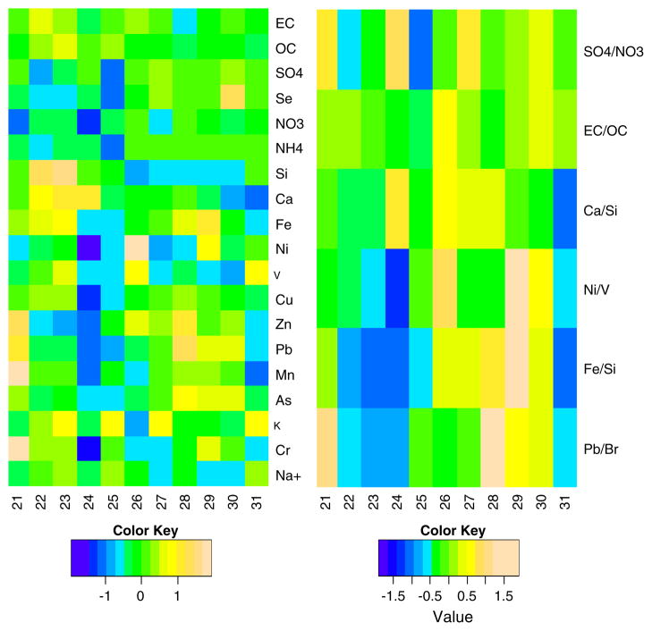
There were 11 clusters that contained only one city. These cities are presented in Table 3 along with heatmaps representing the enrichment factors and normalized ratios at these locations (Fig. 10). Several of these locations exhibit extreme enrichment factors for one or more element as well as extremes in the normalized ratios which helps explains why they do not group with any other sites. On the other hand, a site such as Ironton, OH, does not exhibit extreme values in a single element. However, the relationship between the elements at this site shows some distinct differences as compared to multi-city clusters. The clusters most resembling the pollutant distribution of Ironton are the cities in the Industrial group. These cities have similar Fe/Si ratios and Fe, Mn, Zn and Pb enrichment factors. The Ironton site however, also demonstrates higher K enrichment as well as a higher EC/OC ratio. This suggests that this location is impacted by wood combustion as well as by emissions from industrial processes.
Table 3.
Single city cluster locations.
| Cluster | City | State |
|---|---|---|
| 21 | Birmingham | AL |
| 22 | Phoenix | AZ |
| 23 | Tucson | AZ |
| 24 | Macon | GA |
| 25 | Missoula | MT |
| 26 | New York City (Bronx) | NY |
| 27 | Ironton | OH |
| 28 | Lorain | OH |
| 29 | Youngstown | OH |
| 30 | Pittsburgh | PA |
| 31 | Chester | PA |
Fig. 10.
Heatmaps of single city clusters.
5. Sensitivity analysis
5.1. Data completeness
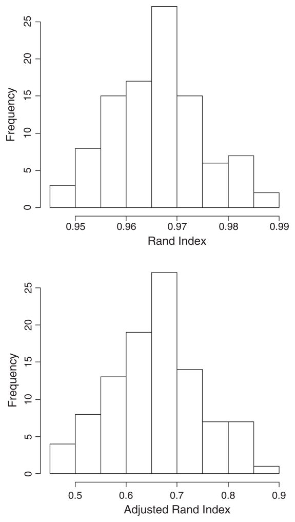
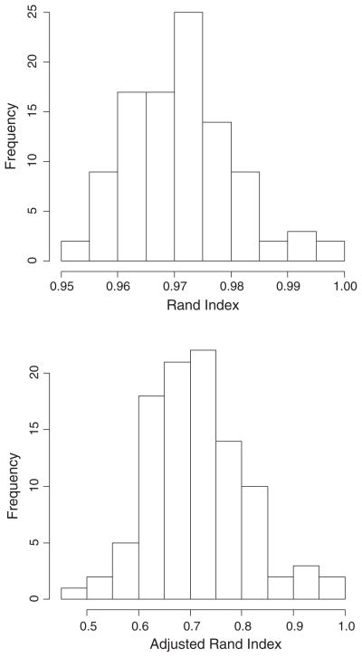
Because each site is represented by a set site mean species proportions we wanted to determine how sensitive the results were to the data points included in calculating the mean. For each site, 20% of the days were randomly excluded and the mean site species proportions were recalculated (Fig. 11). This was repeated 100 times. The solutions obtained were compared to the original one using the Adjusted Rand Index. The mean agreement between the clustering obtained from the analysis of the original data and the test data was adequate (Adjusted Rand Index: 0.66). This test does suggest that there is some sensitivity to the completeness of the original data and supports the choice to require greater than 80% completeness for the cities included in the analysis.
Fig. 11.
Sensitivity analysis; removing 20% of the observations before calculating global mean.
5.2. Sensitivity to site inclusion
The clustering is also subject to which sites are included in the analysis. As such we randomly removed 10% of the sites and repeated the clustering over 100 iterations. We compared the adjusted Rand Index over the 100 iterations, as described above. The results indicate that the solution is somewhat sensitive to which sites are included in the clustering (Fig. 12). Overall, the agreement between the test solutions and the original solution were good with a mean adjusted Rand Index 0.71.
Fig. 12.
Sensitivity analysis; removing 10% of the sites prior to clustering.
5.3. Number of clusters selected
The selection of 31 as an appropriate number of clusters is not an absolutely correct solution. The 31 cluster-solution was compared to other possible solutions encompassing a different number of clusters (k = 1 to 50) using the Adjusted Rand Index. As shown in Fig. 3, for values of k values between 26 and 36 the adjusted Rand Index is higher than 0.70, which suggests that the agreement between solutions is good. This implies that selecting a different value of k would not have yielded dramatically different solutions.
Fig. 3.
Variability of the adjusted Rand Index as a function of the number of clusters selected. (The vertical line represents the number of clusters, k = 31, selected for this study).
5.4. Presence of outlier sites
Because there were 11 single city clusters, we wanted to determine whether removing these sites from the initial data set affected the clustering of the remaining cities. After removing the 11 single city sites, the clustering was re-run. The 20 cluster solution on the reduced dataset is highly comparable to the original clustering with an adjusted rand index of 0.9, and 97% of cases in matched pairs. This confirms that it is not necessary to remove outlier sites prior to clustering.
6. Conclusions
The framework presented here provides a novel tool with which to identify and further classify sites based on their PM2.5 composition. The 31 clusters identified included 21 clusters with 2 or more sites which were classified into four groups. The solution presented is fairly robust to the completeness of data at the sampling sites as well as to the choice of sites to include.
The clusters in the first grouping are located in the Eastern United states. They generally have lower to average enrichment factors for N, V, Si, Ca, Mn and Cr. The urban and rural sites however, are clustering into separate clusters. These sites show average to high concentrations of , Se and As. The enrichment in EC is average to low depending on the urbanization and the enrichment in OC is average. The clusters in the second grouping are located in more industrialized areas. They generally show average to high enrichment factors for metals such as Mn, Pb, Zn, Cr and Fe. The enrichment factors of Si, Ca and Na are average to low. Otherwise, the enrichment factors in this grouping are average. The clusters in the third grouping are located in the western and central United States. The enrichment factor for is very low to average, the enrichment factors of EC and OC are average to high and the Se is average to low. The enrichment factor of is generally high in this grouping. Overall, the species fractions of Zn, Pb, Mn and As are low in this grouping. The last grouping corresponds to clusters located in coastal areas. The enrichment factor of Na+ is average to high, the enrichment factors of Ni and especially the V ones are average to high. The enrichment in and show some variability within these sites as do the Zn, Mn, K and Cr ones.
Further investigation will be conducted to determine whether the associations between long-term health effects and the different types of mixtures provide meaningful information about composition of PM2.5 and/or types of sources posing higher risks. For example, meta-analysis of the long-term health response to PM2.5 could include effect modification by cluster type.
Supplementary Material
Fig. 7.
Group 2, Industrial clusters.
Fig. 8.
Group 3, Western clusters.
Eq. 4.
Enrichment factors.
Acknowledgments
This publication was made possible by USEPA grant RD 83479801. Its contents are solely the responsibility of the grantee and do not necessarily represent the official views of the USEPA. Further, USEPA does not endorse the purchase of any commercial products or services mentioned in the publication. Support was also provided by NIEHS grants ES009825, ES00002 and PO1ES009825 as well as by the Harvard EPA PM Center R-832416.
Authors are acknowledging Drs. Choong Min Kang for the supersite support and Joel Schwartz and his analysis suggestions.
The authors declare they have no actual or potential competing financial interests.
Abbreviations
- NAS
National Academies of Science
- EPA
Environmental Protection Agency
- PM2.5
Particle matter with a diameter of 2.5 μm or less
- EC
Elemental Carbon
- OC
Organic Carbon
- CPC
Condensation Particle Counter
- AQS
Air Quality Standards
Appendix A. Supplementary data
Supplementary data to this article can be found online at http://dx.doi.org/10.1016/j.envint.2013.06.003.
References
- Adame J, Notario A, Villanueva F, Albaladejo J. Application of cluster analysis to surface ozone, NO2 and SO2 daily patterns in an industrial area in Central-Southern Spain measured with a DOAS system. Sci Total Environ. 2012;429:281–91. doi: 10.1016/j.scitotenv.2012.04.032. [DOI] [PubMed] [Google Scholar]
- Agrawal H, Malloy QGJ, Welch WA, Wayne Miller J, Cocker DR. In-use gaseous and particulate matter emissions from a modern ocean going container vessel. Atmos Environ. 2008;42:5504–10. [Google Scholar]
- Ault AP, Gaston CJ, Wang Y, Dominguez G, Thiemens MH, Prather KA. Characterization of the single particle mixing state of individual ship plume events measured at the port of Los Angeles. Environ Sci Technol. 2010;44:1954–61. doi: 10.1021/es902985h. [DOI] [PubMed] [Google Scholar]
- Austin E, Coull B, Thomas D, Koutrakis P. A framework for identifying distinct multipollutant profiles in air pollution data. Environ Int. 2012;45:112–21. doi: 10.1016/j.envint.2012.04.003. [DOI] [PMC free article] [PubMed] [Google Scholar]
- Beaver S, Palazoglu A. A cluster aggregation scheme for ozone episode selection in the San Francisco, CA Bay Area. Atmos Environ. 2006;40:713–25. [Google Scholar]
- Beelen R, Hoek G, Pebesma E, Vienneau D, de Hoogh K, Briggs DJ. Mapping of background air pollution at a fine spatial scale across the European Union. Sci Total Environ. 2009;407:1852–67. doi: 10.1016/j.scitotenv.2008.11.048. [DOI] [PubMed] [Google Scholar]
- Bell ML, Dominici F, Samet JM. A meta-analysis of time-series studies of ozone and mortality with comparison to the national morbidity, mortality, and air pollution study. Epidemiology. 2005;16:436. doi: 10.1097/01.ede.0000165817.40152.85. [DOI] [PMC free article] [PubMed] [Google Scholar]
- Bell ML, Dominici F, Ebisu K, Zeger SL, Samet JM. Spatial and temporal variation in PM2. 5 chemical composition in the United States for health effects studies. Environ Health Perspect. 2007;115:989. doi: 10.1289/ehp.9621. [DOI] [PMC free article] [PubMed] [Google Scholar]
- Chuang KJ, Chan CC, Su TC, Lee CT, Tang CS. The effect of urban air pollution on inflammation, oxidative stress, coagulation, and autonomic dysfunction in young adults. Am J Respir Crit Care Med. 2007;176:370. doi: 10.1164/rccm.200611-1627OC. [DOI] [PubMed] [Google Scholar]
- Comrie AC. An all-season synoptic climatology of air pollution in the US–Mexico border region. Prof Geogr. 1996;48:237–51. [Google Scholar]
- Cormack RM. A review of classification. J R Stat Soc Ser A (Gen) 1971;134:321–67. [Google Scholar]
- de Foy B, et al. Sources of nickel, vanadium and black carbon in aerosols in Milwaukee. Atmos Environ. 2012;59:294–301. [Google Scholar]
- Dockery DW, Pope CA, III, Xu X, Spengler JD, Ware JH, Fay ME, et al. An association between air pollution and mortality in six US cities. N Engl J Med. 1993;329:1753–9. doi: 10.1056/NEJM199312093292401. [DOI] [PubMed] [Google Scholar]
- Dominici F, Peng RD, Barr CD, Bell ML. Protecting human health from air pollution: shifting from a single-pollutant to a multipollutant approach. Epidemiology. 2010;21:187. doi: 10.1097/EDE.0b013e3181cc86e8. [DOI] [PMC free article] [PubMed] [Google Scholar]
- Flemming J, Stern R, Yamartino R. A new air quality regime classification scheme for O3, NO2, SO2 and PM10 observations sites. Atmos Environ. 2005;39:6121–9. [Google Scholar]
- Gao F, Barchowsky A, Nemec AA, Fabisiak JP. Microbial stimulation by Mycoplasma fermentans synergistically amplifies IL-6 release by human lung fibroblasts in response to residual oil fly ash (ROFA) and nickel. Toxicol Sci. 2004;81:467. doi: 10.1093/toxsci/kfh205. [DOI] [PMC free article] [PubMed] [Google Scholar]
- Hartigan J, Wong M. A k-means clustering algorithm. J R Stat Soc Ser C. 1979;28:100–8. [Google Scholar]
- Henry RC, Kim BM. Extension of self-modeling curve resolution to mixtures of more than three components: Part 1. Finding the basic feasible region. Chemom Intell Lab Syst. 1990;8:205–16. [Google Scholar]
- Hubert L, Arabie P. Comparing partitions. J Classif. 1985;2:193–218. [Google Scholar]
- Isakson J, Persson T, Selin Lindgren E. Identification and assessment of ship emissions and their effects in the harbour of Göteborg, Sweden. Atmos Environ. 2001;35:3659–66. [Google Scholar]
- Jain AK, Murty MN, Flynn PJ. Data clustering: a review. ACM Comput Surv (CSUR) 1999;31:264–323. [Google Scholar]
- Janssen NAH, Schwartz J, Zanobetti A, Suh HH. Air conditioning and source-specific particles as modifiers of the effect of PM (10) on hospital admissions for heart and lung disease. Environ Health Perspect. 2002;110:43. doi: 10.1289/ehp.0211043. [DOI] [PMC free article] [PubMed] [Google Scholar]
- Jerrett M, Burnett RT, Ma R, Pope CA, III, Krewski D, Newbold KB, et al. Spatial analysis of air pollution and mortality in Los Angeles. Epidemiology. 2005;16(6):727–36. doi: 10.1097/01.ede.0000181630.15826.7d. [DOI] [PubMed] [Google Scholar]
- Kavouras IG, Koutrakis P, Tsapakis M, Lagoudaki E, Stephanou EG, Von Baer D, et al. Source apportionment of urban particulate aliphatic and polynuclear aromatic hydrocarbons (PAHs) using multivariate methods. Environ Sci Technol. 2001;35: 2288–94. doi: 10.1021/es001540z. [DOI] [PubMed] [Google Scholar]
- Kim BM, Henry RC. Extension of self-modeling curve resolution to mixtures of more than three components: Part 2. Finding the complete solution. Chemom Intell Lab Syst. 1999;49:67–77. [Google Scholar]
- Kim SB, Temiyasathit C, Chen VCP, Park SK, Sattler M, Russell AG. Characterization of spatially homogeneous regions based on temporal patterns of fine particulate matter in the continental United States. J Air Waste Manage Assoc. 2008;58:965–75. doi: 10.3155/1047-3289.58.7.965. [DOI] [PubMed] [Google Scholar]
- Koutrakis P, Spengler JD. Source apportionment of ambient particles in Steubenville, OH using specific rotation factor analysis. Atmos Environ. 1987;21:1511–9. [1967] [Google Scholar]
- Koutrakis P, Sax SN, Sarnat JA, Coull B, Demokritou P, Oyola P, et al. Analysis of PM 10, PM 2. 5, and PM 2. 5–10 Concentrations in Santiago, Chile, from 1989 to 2001. J Air Waste Manage Assoc. 2005;55:342–51. doi: 10.1080/10473289.2005.10464627. [DOI] [PubMed] [Google Scholar]
- Laden F, Neas LM, Dockery DW, Schwartz J. Association of fine particulate matter from different sources with daily mortality in six US cities. Environ Health Perspect. 2000;108:941. doi: 10.1289/ehp.00108941. [DOI] [PMC free article] [PubMed] [Google Scholar]
- Lee JH, Hopke PK. Apportioning sources of PM 2.5 in St. Louis, MO using speciation trends network data. Atmos Environ. 2006;40:360–77. [Google Scholar]
- Lefohn AS, Shadwick D, Oltmans SJ. Characterizing changes in surface ozone levels in metropolitan and rural areas in the United States for 1980–2008 and 1994–2008. Atmospheric Environment. 2010;44(39):5199–210. [Google Scholar]
- Lippmann M, Ito K, Hwang JS, Maciejczyk P, Chen LC. Cardiovascular effects of nickel in ambient air. Environ Health Perspect. 2006;114:1662. doi: 10.1289/ehp.9150. [DOI] [PMC free article] [PubMed] [Google Scholar]
- Maitra R, Peterson AD, Ghosh AP. A systematic evaluation of different methods for initializing the k-means clustering algorithm. IEEE Trans Knowl Data Eng. 2010 [Google Scholar]
- Mar TF, Norris GA, Koenig JQ, Larson TV. Associations between air pollution and mortality in Phoenix, 1995–1997. Environ Health Perspect. 2000;108:347. doi: 10.1289/ehp.00108347. [DOI] [PMC free article] [PubMed] [Google Scholar]
- Mauderly JL, Burnett RT, Castillejos M, Özkaynak H, Samet JM, Stieb DM, et al. Is the air pollution health research community prepared to support a multipollutant air quality management framework? Inhal Toxicol. 2010;22:1–19. doi: 10.3109/08958371003793846. [DOI] [PubMed] [Google Scholar]
- National Research Council (US), Committee on Air Quality Management in the United States. Air quality management in the united states. Natl Academy Pr; 2004. [Google Scholar]
- O’Neill MS, Veves A, Zanobetti A, Sarnat JA, Gold DR, Economides PA, et al. Diabetes enhances vulnerability to particulate air pollution-associated impairment in vascular reactivity and endothelial function. Circulation. 2005;111:2913–20. doi: 10.1161/CIRCULATIONAHA.104.517110. [DOI] [PubMed] [Google Scholar]
- Paatero P, Tapper U. Positive matrix factorization: a non-negative factor model with optimal utilization of error estimates of data values. Environmetrics. 1994;5:111–26. [Google Scholar]
- Pakalapati S, Beaver S, Romagnoli JA, Palazoglu A. Sequencing diurnal air flow patterns for ozone exposure assessment around Houston, Texas. Atmos Environ. 2009;43:715–23. [Google Scholar]
- Peltier RE, Lippmann M. Residual oil combustion: 2. Distributions of airborne nickel and vanadium within New York City. J Expo Sci Environ Epidemiol. 2009;20:342–50. doi: 10.1038/jes.2009.28. [DOI] [PubMed] [Google Scholar]
- Pope CA, Dockery DW. Health effects of fine particulate air pollution: lines that connect. J Air Waste Manage Assoc. 2006;56:709–42. doi: 10.1080/10473289.2006.10464485. [DOI] [PubMed] [Google Scholar]
- Pope C, 3rd, Thun MJ, Namboodiri MM, Dockery DW, Evans JS, Speizer FE, et al. Particulate air pollution as a predictor of mortality in a prospective study of US adults. American journal of respiratory and critical care medicine. 1995;151:669–74. doi: 10.1164/ajrccm/151.3_Pt_1.669. [DOI] [PubMed] [Google Scholar]
- Punj G, Stewart DW. Cluster analysis in marketing research: review and suggestions for application. J Mark Res. 1983;20:134–48. [Google Scholar]
- Rand WM. Objective criteria for the evaluation of clustering methods. J Am Stat Assoc. 1971;66:846–50. [Google Scholar]
- Samet JM, Dominici F, Curriero FC, Coursac I, Zeger SL. Fine particulate air pollution and mortality in 20 U.S. cities, 1987–1994. N Engl J Med. 2000;343:1742–9. doi: 10.1056/NEJM200012143432401. [DOI] [PubMed] [Google Scholar]
- Schwartz J, Laden F, Zanobetti A. The concentration–response relation between PM (2.5) and daily deaths. Environ Health Perspect. 2002;110:1025. doi: 10.1289/ehp.021101025. [DOI] [PMC free article] [PubMed] [Google Scholar]
- Steinley D. Properties of the Hubert–Arabie Adjusted Rand Index. Psychol Methods. 2004;9:386. doi: 10.1037/1082-989X.9.3.386. [DOI] [PubMed] [Google Scholar]
- Steinley D. K-means clustering: a half-century synthesis. Br J Math Stat Psychol. 2006;59:1–34. doi: 10.1348/000711005X48266. [DOI] [PubMed] [Google Scholar]
- Taubman B, Hains J, Thompson A, Marufu L, Doddridge B, Stehr J, et al. Aircraft vertical profiles of trace gas and aerosol pollution over the mid-Atlantic United States: statistics and meteorological cluster analysis. J Geophys Res. 2006;111:D10S07. [Google Scholar]
- Thurston GD, Spengler JD. A quantitative assessment of source contributions to inhalable particulate matter pollution in metropolitan Boston. Atmospheric Environment. 1985;19(1967):9–25. [Google Scholar]
- Thurston GD, Ito K, Mar T, Christensen WF, Eatough DJ, Henry RC, et al. Workgroup report: workshop on source apportionment of particulate matter health effects—intercomparison of results and implications. Environ Health Perspect. 2005;113:1768. doi: 10.1289/ehp.7989. [DOI] [PMC free article] [PubMed] [Google Scholar]
- U.S. EPA. The multi-pollutant report: technical concepts and examples. Washington, DC: U.S. EPA; 2008. [Google Scholar]
- U.S. EPA. Location of US Facilities. U.S. Environmental Protection Agency; 2011. Jan 12th, Retrieved September 24th 2012, from http://www.epa.gov/sectors/sectorinfo/sectorprofiles/ironsteel/map.html. [Google Scholar]
- Vedal S, Kaufman JD. What does multi-pollutant air pollution research mean? Am J Respir Crit Care Med. 2011;183:4. doi: 10.1164/rccm.201009-1520ED. [DOI] [PubMed] [Google Scholar]
- Ward JH. Hierarchical grouping to optimize an objective function. J Am Stat Assoc. 1963;58:236–44. [Google Scholar]
- Zanobetti A, Schwartz J. Temperature and mortality in nine US cities. Epidemiology. 2008;19:563–70. doi: 10.1097/EDE.0b013e31816d652d. [DOI] [PMC free article] [PubMed] [Google Scholar]
- Zanobetti A, Schwartz J, Samoli E, Gryparis A, Touloumi G, Atkinson R, et al. The temporal pattern of mortality responses to air pollution: a multicity assessment of mortality displacement. Epidemiology. 2002;13:87–93. doi: 10.1097/00001648-200201000-00014. [DOI] [PubMed] [Google Scholar]
- Zhou J, Ito K, Lall R, Lippmann M, Thurston G. Time-series analysis of mortality effects of fine particulate matter components in Detroit and Seattle. Environ Health Perspect. 2011;119:461. doi: 10.1289/ehp.1002613. [DOI] [PMC free article] [PubMed] [Google Scholar]
Associated Data
This section collects any data citations, data availability statements, or supplementary materials included in this article.


