Joint tuning for direction of motion and binocular disparity in macaque MT is largely separable

Abstract

Neurons in sensory cortical areas are tuned to multiple dimensions, or features, of their sensory space. Understanding how single neurons represent multiple features is of great interest for determining the informative dimensions of the neurons' response, the decoding algorithms appropriate for extracting this information from the neuronal population, and for determining where specific transformations occur along the visual hierarchy. Despite the established role of cortical area MT in judgments of motion and depth, it is not known how individual neurons jointly encode the two dimensions. We investigated the joint tuning of individual MT neurons for two visual features: direction of motion and binocular disparity, an important depth cue. We found that a separable, multiplicative combination of tuning for the two features can account for more than 90% of the variance in the joint tuning function for over 91% of MT neurons. These results suggest 1) that each feature can be read out independently from MT by simply averaging across the population without regard to the other feature and 2) that the inseparable representations seen in subsequent areas, such as MST, must be computed beyond MT. Intriguingly, we found that the remaining nonseparable component of the joint tuning function often manifested as small but systematic changes in the neurons' preferences for one feature as the other one was varied. We believe this reflects the local columnar organization of tuning for direction and binocular disparity in MT, indicating that joint tuning may provide a new tool with which to probe functional architecture.

the spike rates of most cortical sensory neurons are modulated by multiple stimulus features. For example, many V1 neurons are sensitive to the orientation of a contour and to its contrast, length, or direction of motion. If such a neuron's preference for orientation does not change as a function of change in the other stimulus features, its preference for orientation is invariant and represented in a “separable” manner from other features. A separable representation allows for simple averaging across irrelevant stimulus dimensions for accurate read-out of the feature of interest (Grunewald and Skoumbourdis 2004; Heeger 1987; Qian and Andersen 1997). However, an inseparable combination of two features can result in more complex selectivity. For example, speed sensitivity that is invariant to spatial frequency arises in MT from the inseparable combination of V1 inputs that are sensitive to particular combinations of spatial and temporal frequency responses (Priebe et al. 2006). This inseparable representation makes MT neurons informative about speed across a variety of images but not informative about the spatial frequency content of the image, since their preferred spatial frequency changes as temporal frequency varies. The latter information is best extracted from V1. Similar inseparable feature combinations endow MT neurons with sensitivity to spatial velocity gradients and relative depth (Krug and Parker 2011; Treue and Andersen 1996). Furthermore, the separability of tuning for each feature with respect to time can reveal interesting response dynamics such as those that have been observed in earlier parts of the visual stream (e.g., Allen and Freeman 2006; Bredfeldt and Ringach 2002; Malone and Ringach 2008; Mazer et al. 2002; Menz and Freeman 2003) and in MT for complex motion stimuli (Pack and Born 2001; Pack et al. 2004; Smith et al. 2005).

In addition to being speed selective, most MT neurons are also selective for the direction of moving stimuli and binocular disparity, an important depth cue (Born and Bradley 2005). Although it is well established that MT neurons are involved in decisions during motion and depth tasks (Britten et al. 1996; DeAngelis et al. 1998; Salzman et al. 1992; Uka and DeAngelis 2004), how these features are jointly encoded by individual neurons is not fully understood. Responses to the combination of these two features can be nonlinear when several transparent surfaces are overlaid in an MT neuron's receptive field. For example, binocular disparity cues can reduce inhibition by motion in the null direction (Bradley et al. 1995) and thus facilitate surface segregation (Bradley et al. 1998). Interactions between the binocular disparity of two transparent surfaces can also yield sensitivity to relative depth (Krug and Parker 2011). However, the basic interaction of these two features in a single nontransparent stimulus, the complete joint tuning function, has not been described. Notably, in MST, a major target of MT projections (Maunsell and Van Essen 1983a; Ungerleider and Desimone 1986), the representation of these two features is inseparable such that the preferred direction of many neurons reverses when the depth plane of the visual stimulus is changed from near to far, which may allow for explicit encoding of self-motion (Roy and Wurtz 1990; Roy et al. 1992). It is not known whether this computation is performed within MST or there exist MT neurons with sufficiently inseparable responses that can be pooled to achieve this representation.

Neurons in V1, a major source of cortical input to MT, represent these features separably such that their preferences for direction do not change as binocular disparity is varied (Grunewald and Skoumbourdis 2004). However, it is unlikely that MT simply inherits its joint tuning for direction and binocular disparity, along with a separable joint representation, directly from its V1 inputs. Whereas the basic properties of direction selectivity in MT are well accounted for by the properties of their V1 inputs (Hedges et al. 2011; Pack et al. 2006; Shadlen et al. 1996), the same is not true for binocular disparity (Cumming and DeAngelis 2001). Simply pooling V1 inputs cannot reproduce either the shape or range of the disparity tuning curves typically found in MT. Instead, it is likely that the tuning for binocular disparity is conveyed to MT by a distinct anatomic pathway that involves V2 (Ponce et al. 2008).

It therefore remains unclear precisely how MT neurons combine tuning for the two features with which they are principally concerned. To address this, we measured the complete joint tuning function for direction and binocular disparity of MT neurons in three alert macaque monkeys.

MATERIALS AND METHODS

Animals

Three adult male macaque monkeys (N, P, and Q), Macaca mulatta, were seated comfortably in custom chairs (Crist Instruments) during all experiments. Two of the animals, monkeys N and P, had previously been trained to detect a speed change in stimuli presented at a range of binocular disparities. The third, monkey Q, had been trained to detect the onset of coherent motion or depth in noisy stimuli.

Before electrophysiological recordings, we implanted in each animal a custom titanium head post, two scleral search coils for monitoring eye positions and vergence, and a Cilux recording cylinder (Crist Instruments) to protect the craniotomy used to access MT. In monkeys N and P the craniotomy was centered 3 mm posterior and 15 mm lateral relative to ear bar zero; in monkey Q the craniotomy was centered 17 mm anterior and 15 mm lateral to ear bar zero, allowing for an anterior approach. This animal also had chronically implanted cryoloops in the ipsilateral lunate sulcus, but these were not used in the course of the experiments described in this report. All animal procedures complied with the National Institutes of Health Guide for the Care and Use of Laboratory Animals and were approved by the Harvard Medical Area Standing Committee on Animals.

Visual Stimuli and Task

Stimuli consisted of high-contrast moving random dot patches presented on a black background on a CRT monitor with a resolution of 1,024 × 768 pixels (17.8 pixels/deg) and refresh rate of 100 Hz, located 41 cm in front of the animal. All stimuli were drawn using the Cogent toolbox in MATLAB. The animals were trained to fixate their gaze on a central spot displayed in the plane of the monitor screen with positive reinforcement using liquid rewards. The monkeys were rewarded for maintaining fixation for the presentation of 2 to 4 stimuli, each of which was presented for 400–500 ms. Each moving stimulus presented to monkeys N and P was preceded by a stationary dot patch. Stimuli consisted of round dot patches that were drawn at a range of binocular disparities and directions of motion. The binocular disparity of each stimulus was specified by drawing each dot twice, once in red and once in blue, and changing each dot pair's horizontal offset according to the specified binocular disparity value. Dots in the plane of fixation (zero binocular disparity) were drawn as a combination of the blue and red values, which appeared magenta. During all experiments, there were several dozen dots drawn at zero disparity in an annulus around the fixation target to aid the animal in maintaining vergence angle in the plane of fixation (Nguyenkim and DeAngelis 2003).

The monkeys viewed the screen through red/blue anaglyphs (Kodak gelatin filters nos. 29 and 47) so that only one set of dots was visible to each eye. Crossover of the image between the two eyes, as viewed through the filters, was measured to be less than 3%. Dots were presented at a spatial density of 1.5 dots/deg², with 150-ms lifetime and 100% coherence (i.e., there were no noise dots, but the dots flickered because of their limited lifetime). Monkeys N and P viewed a stimulus set that consisted of 7 binocular disparities, spaced 0.4° apart (−1.2°, −0.8°, −0.4°, 0°, 0.4°, 0.8°, 1.2°) and 8 directions of motion spaced 45° apart (0°, 45°, 90°, 135°, 180°, 225°, 270°, 315°). To obtain a more finely sampled joint tuning function, monkey Q was presented with a stimulus set that consisted of more finely spaced steps of both features that were centered on the preferred direction and binocular disparity of the neuron under study, which were estimated by hand mapping. In this animal, directions were spaced 30° apart and the binocular disparities were spaced 0.2° apart. In addition, in this animal we often sampled more coarsely around the null values of each feature. Therefore, the joint tuning functions collected from monkey Q were often not uniformly sampled (but the null value was always included); all neurons from monkey N and P were tested with uniformly sampled directions and binocular disparities.

Electrophysiological Recording

Single neurons were selected for study if they were determined to be in area MT by a combination of anatomical and functional properties and if they were modulated by the direction of motion of moving stimuli. Each neuron's size and speed tuning were estimated by hand mapping, and the diameter of the stimulus was set to be equal to either the receptive field's eccentricity or the peak of the neuron's area summation curve, whichever was smaller. The stimulus's speed was set to be the maximally responsive value within a range of 4–25°/s. Joint tuning functions were considered for analysis if the neurons were significantly modulated by both features (P < 0.05, ANOVA) at the preferred value of the other feature and there were at least five repetitions of each stimulus combination (median = 25). Single-unit isolation was enforced with offline principal components analysis.

Analysis

We averaged spike rates across trials in a 200- to 350-ms window, depending on the duration of stimulus presentation for each experiment (which changed once in the course of this study). The start of the time window was chosen to only include the stationary, posttransient response.

Change in tuning preferences.

To determine whether the preferences of the neuron changed as we varied the stimulus along the other feature dimension, we fit parametric functions to each tuning curve within the joint tuning function (e.g., one direction tuning curve for every binocular disparity tested). The direction tuning curves were fit with a von Mises function, which is the circular approximation of a Gaussian distribution, of the form

$$R_{\text{dir}}=R_0+A{e}^{b\cos \left(\theta -{\theta }_0\right)},$$ (1)

where the response to each direction, R_dir, is a function of the stimulus direction, θ, and R₀ is the baseline firing rate, A the amplitude, b the tuning bandwidth, and θ₀ the preferred direction. Disparity tuning curves were fit with Gabor functions (DeAngelis and Uka 2003) of the form

$$R_{\text{disp}}=R_0+A{e}^{-0.5\left[\left(d-d_0\right){}^2/{\sigma }^2\right]}\times \cos \left[2\pi f\left(d-d_0\right)+\varphi \right],$$ (2)

where the response to each disparity, R_disp, is a function of the stimulus disparity, d, and R₀ corresponds to the baseline firing rate, A the amplitude, d₀ the Gaussian center, σ the Gaussian width, f the disparity frequency, and ϕ the phase. Fitting of both functions was performed using least-squares minimization in MATLAB. The location of the peak of the fitted functions specified the preferred direction and binocular disparity. To determine whether changes in tuning preferences were statistically significant, we estimated confidence intervals on our estimate of the preferred value with a bootstrap procedure. For each neuron, spike rates from individual trials were resampled with replacement, preserving information about stimulus direction and binocular disparity, to generate a new mean response for each stimulus tested. The resultant tuning curves were then fit with their respective functions and the preferred values estimated from the fit, as with the original data. This was repeated 2,000 times to give 95% confidence intervals for each estimate of the preferred direction and binocular disparity. The null hypothesis that the preferred value was the same between two conditions was rejected at the 0.05 level if their confidence intervals did not overlap.

Separable predictions.

Additive and multiplicative separable predictions of each neuron's joint tuning function were generated using methods described by Peña and Konishi (2001). For these predictions, the raw mean responses from the joint tuning function of each neuron were used, without employing the parametric functions fitted to the data. We required each neuron to be significantly modulated by binocular disparity and direction for at least 3 values of the other feature to be included in these analyses, which led us to exclude 23 of 94 neurons because they were too narrowly tuned.

We generated the multiplicative prediction with the use of singular value decomposition (SVD). This method decomposes a matrix, in this case the joint tuning function, into a weighted sum of the products of two independent vectors, called singular vectors. The weight for each product is given by the singular values, which are ordered in a diagonal matrix. They are ordered by their contribution to the original data matrix such that the first one corresponds to the largest component of the data. Therefore, the first left and right singular vectors returned by SVD represent the best separable approximations to the underlying direction and binocular disparity tuning curves. The product of the first singular value and the first left and right singular vectors is the best prediction of a multiplicative separable combination of the two tuning curves, in the least-squared sense (Ahrens et al. 2008).

The complete multiplicative model is then given by

$$M_{\text{mult}}\left(i,j\right)=k+\sigma U\left(i\right)V{\left(j\right)}^T,$$ (3)

where the first term is a constant offset represented by k, which was optimized by minimizing the sum of the squared singular values other than the first one in the SVD of M − k. The second term represents the multiplicative interaction between binocular disparity and direction tuning functions, denoted by U and V, respectively, and σ is the first singular value. U and V are the first left and right singular vectors returned by the SVD procedure.

The additive model was described by

$$M_{\text{add}}\left(i,j\right)=\mu +F\left(i\right)+G\left(j\right),$$ (4)

where μ is a constant offset corresponding to the mean response across the entire joint tuning function and F and G represent the binocular disparity and direction tuning functions, which were obtained by averaging the rows and columns of M − μ, respectively.

Small changes in tuning preferences.

We quantified the relationship between changes in stimulus properties in one feature dimension and the small observed changes in each neuron's preferences in the other feature, as described in results. The preferred direction and binocular disparity were estimated from the fitted parametric functions. To estimate changes in the preferred stimulus for one feature (e.g., direction), we required that each neuron be significantly modulated (P < 0.05 in an ANOVA) by that feature for at least four values of the other feature (e.g., binocular disparity). This ensured that there were always at least three data points for the linear fit to the rate of change in the preferred feature (see results). Furthermore, these responses had to be well fit by their respective parametric function (R² > 0.85). Of the 94 recorded neurons, 78 met both of these criteria for direction tuning, 37 for binocular disparity tuning, and 34 for both. There were fewer eligible neurons that met these criteria for binocular disparity because neurons tended to not be significantly modulated by binocular disparity at values of direction near to the null value, where neuronal responses approached noise levels.

RESULTS

We recorded from 94 well-isolated MT neurons in three awake macaque monkeys (32 in monkey N, 35 in monkey P, and 27 in monkey Q) while they fixed their gaze on a central point on a computer screen. An example stimulus set used in one of our experiments is shown in Fig. 1A. Figure 1, B and C, shows simulated data highlighting some differences between a separable and inseparable representation of two features. In a heat map representation of the joint tuning function for two stimulus features that each have a single-peaked tuning function, a separable combination appears as an ellipse that is either circular or vertically or horizontally oriented with no change in the location of the peak along the rows or the columns (Fig. 1B). In contrast, any tilt of the ellipse reflects inseparability in the combination of the two features and indicates a change in direction and binocular disparity preferences as the stimulus is varied in the other feature (Fig. 1C). It is important to note that this is not the only way a neuron may exhibit inseparable tuning. It is possible, for example, for the preferred direction to change sharply when the binocular disparity is changed from near to far values rather than gradually as indicated by the tilt. Such erratic changes in tuning would appear as random hot spots in different columns and rows in the joint tuning maps.

Fig. 1.

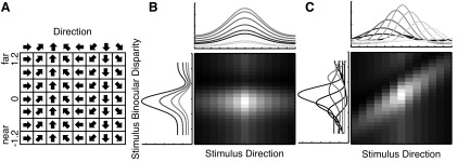
Experimental design and hypothesis. A: sample stimulus set used in one of our experiments. The stimuli consisted of the matrix populated by all combinations of the tested directions of motion and binocular disparities. B: simulated joint tuning function of a separable combination of direction and binocular disparity. Tuning curves in the marginal plots show several tuning curves sampled at different values of the other feature. Although the response magnitude changes as feature values vary away from the preferred, the preferred direction and binocular disparity do not change. C: simulated joint tuning function for one type of inseparable combination of direction and binocular disparity (same conventions as in B). In addition to the change in magnitude, the preferred direction and binocular disparity change as the other feature is varied in the visual stimulus. To read out information about the direction of a moving stimulus from this neuron, it is also necessary to know the binocular disparity of the stimulus.

Change in Tuning Preferences

Figure 2 shows the joint tuning function of a representative MT neuron. The top marginal panel shows direction tuning curves obtained when the stimulus was presented at each binocular disparity. The left marginal panel shows the same data arranged to show the binocular disparity tuning collected at different directions of motion. The same information is shown again in the two-dimensional (2-D) heat map, in which the entire joint tuning function (the response to each combination of direction and binocular disparity) is shown. The direction tuning curves show that while the overall firing rate changes at different binocular disparities, the direction preferences of this cell remain virtually identical. The results are similar for the binocular disparity tuning as stimulus direction is changed. This is also evident in the 2-D joint tuning function from the consistent location of the peaks between the rows and columns (compare to Fig. 1C).

Fig. 2.

Example joint tuning function from a single neuron. The joint tuning curve of a neuron recorded from monkey Q is shown in the two-dimensional (2-D) heat map. The hatched region indicates stimulus directions that were not sampled for this neuron because of the nonuniform sampling of directions in neurons recorded from monkey Q (see materials and methods). The luminance scale indicates the firing rate in spikes per second. The individual direction and binocular disparity tuning curves are shown in top and left marginal panels, respectively. The values to the right of each plot indicate the values of the other feature for each tuning curve. The direction tuning curves are shown with the best-fit von Mises functions, and the binocular disparity tuning curves are shown with the best-fit Gabor functions. The binocular disparity tuning curve measured at the preferred direction (120°) and the direction tuning curve at the preferred binocular disparity (0.8°) are shown with the SE around each data point; the SE is smaller than most data points for both tuning curves. This neuron was significantly modulated by stimulus direction when the stimulus was at all binocular disparities and significantly modulated by binocular disparity at all tested stimulus directions.

Six more example neurons are shown in Fig. 3 to highlight some of the common features found in the population. In the example neurons in Fig. 3, A–D, the preferred direction, i.e., the location of the peak response in each column, does not change much as the stimulus binocular disparity is varied. The same is true for the preferred disparity, i.e., the peak in each row, as the stimulus direction is varied. This is consistent with a largely separable combination of the two features. The neurons in Fig. 3, E and F, exhibit some of the largest changes in preferences in our recorded population, yet the preferences for binocular disparity and direction change only slightly as the stimulus parameters are changed (e.g., there are no reversals in preferred direction, as has been found in MST; Roy et al. 1992). We quantified the changes in preferred direction and binocular disparity from the von Mises and Gabor functions, respectively, that were fit to the data. The largest deviation from the preferred direction (as measured at the preferred binocular disparity) for the neuron in Fig. 3E was 20°, and the largest deviation in preferred binocular disparity (as measured at the preferred direction) was 0.2°, although neither of these values reached statistical significance, as determined by a resampling procedure (see materials and methods). For the neuron in Fig. 3F, these changes were 20° for direction of motion and 0.4° for binocular disparity, the latter of which was statistically significant (P < 0.05, bootstrap procedure).

Fig. 3.

Additional joint tuning function examples. A–F: 2-D joint tuning functions from 6 additional neurons (same conventions as Fig. 2). Cross-validated R² values between the data and the multiplicative (R_m²) and additive (R_a²) predictions are shown at top right for each neuron (see results).

Across the population, we found that few neurons exhibited a significant change in preferred direction between stimulus presentations at the preferred and null binocular disparities. This analysis required that neurons remained significantly tuned to direction at the null binocular disparity, so not all neurons could be included. Of the 77 neurons that were significantly tuned to direction at the null binocular disparity, only 17 exhibited a significant change in preferred direction. Across all 77 neurons, the median change in preferred direction was 4.2°, and for the subset of 17 neurons that showed a significant change, the median change was 11.6°. There were far fewer cells that continued to be significantly modulated by binocular disparity at the null direction of motion. Of the 14 neurons that remained significantly tuned at the null direction, 3 exhibited a significant change in preferred disparity. No neurons exhibited a significant change in preferred disparity at the direction perpendicular to the preferred. The median change for all 14 neurons was 0.13°. These changes are small enough that they fall within the resolution with which these tuning curves are typically sampled.

Separability

The small changes in preferences for either feature suggest that tuning for direction and binocular disparity is largely separable. A separable representation of two features can result from either an additive or multiplicative combination of the feature responses. We quantitatively determined the degree to which each separable model can account for our data by generating an additive and a multiplicative prediction for the joint tuning function for each neuron using methods described by Peña and Konishi (2001). We used half of each neuron's data to generate the predictions, which we then compared with the remaining half of the data to give cross-validated R² values.

We generated the multiplicative prediction for a strictly separable combination of direction and binocular disparity using SVD (see materials and methods). Briefly, SVD factors a matrix into two sets of sorted orthonormal vectors. These are sorted and weighted by the singular values such that the first one has the highest explanatory power for the original matrix. Indeed in our data, the first singular value dominated the explained variability in the data with a median explanatory power of 99%. The mean normalized singular values are shown in Fig. 4D. Taking the product of the first singular value and the first left and right singular vectors gives the best separable multiplicative prediction of the original data in the least-squares sense. We also included an additional offset term in this model, which was optimized for each neuron. An F-test confirmed that the additional offset parameter justifiably improved the fit to the original data (P < 0.01 for all neurons).

Fig. 4.

Multiplicative and additive separable predictions for a sample joint tuning function. A: the joint tuning function of the same neuron as in Fig. 2. B: the multiplicative prediction, with the R² between the prediction and the original data shown at top right. C: the additive prediction and the accompanying R² value. D: the average singular values, normalized to the first singular value (SV) for each neuron.

The joint tuning function and the prediction generated by the multiplicative model for the example neuron shown in Fig. 2 are shown in Fig. 4, A and B. In this case, the R² value between the data and the multiplicative prediction was 0.99, indicating that it captured 99% of the variance of the joint tuning function. For reference, the proportion of variance (R²) captured by the multiplicative prediction for the simulated joint tuning function shown in Fig. 1C was 0.66. Across the population, we found that the mean R² value between each neuron's joint tuning function and the multiplicative prediction was 0.96 (Fig. 5A).

Fig. 5.

Population R² values for the multiplicative and additive predictions. A: a comparison of the cross-validated R² values for the relationship between the data and the multiplicative and additive predictions for the joint tuning functions of all included neurons. B: the cross-validated R² values between the data and the additive and multiplicative predictions for the direction-time tuning function (same conventions as in A). C: the cross-validated R² values between the data and the additive and multiplicative predictions for the binocular disparity-time tuning function (same conventions as in A).

We compared these predictions with those from an additive model, in which the underlying direction and disparity tuning functions were added together, point by point, to generate a prediction. For the example neuron in Figs. 2 and 4, the additive prediction accounted for 93% of the variance (Fig. 4C). Across the population this model predicted the data well but significantly less so than the multiplicative model, with a mean R² value of 0.91 (Fig. 5A), which was slightly but significantly worse than the multiplicative prediction as determined by a pairwise comparison of the R² values (mean difference = −0.05, P ≪ 0.01, paired t-test on Fisher's z-transformed R² values). It is important to note that the R² values from the two models could be compared directly because the multiplicative model did not include an additive term and therefore had the same number of parameters as the additive model. Qualitatively, the additive model tended to fail when the stimulus was close to the null values for direction and disparity, usually by overestimating the response and thereby predicting the neuron would be more tuned at these null values than in the measured response.

We also examined the stability of direction and binocular disparity tuning throughout the stimulus presentation period by computing the separability of direction and binocular disparity with respect to time (Fig. 5, B and C). For each neuron we generated a direction-time matrix by computing direction tuning at the preferred binocular disparity in a sliding, nonoverlapping 50-ms time window beginning at motion onset and ending when the stimulus was no longer on the screen. We measured binocular disparity tuning at the preferred direction in the same manner. We then made separable multiplicative and additive predictions for each of these matrices using the methods described for the joint tuning function. The direction-time function was better described by a multiplicative than additive model (mean pairwise difference in R² values = 0.16 P ≪ 0.01, paired t-test on Fisher's z-transformed R² values), but the two predictions performed similarly for the binocular disparity-time function (mean difference = 0.01, P < 0.01, paired t-test on Fisher's z-transformed R² values). The mean R² value for the multiplicative separable prediction for direction tuning with respect to time was 0.88, indicating that direction tuning was largely independent of time, as has previously been shown for MT neurons in response to either moving random dots or fields of bars moving perpendicularly to their orientation axis (Pack et al. 2001, 2004). Binocular disparity tuning was slightly more dependent on time with a mean R² value of 0.84, which was significantly different from the mean R² value for the direction-time prediction (P < 0.01, paired t-test on Fisher's z-transformed R² values). Since these predictions were made for data computed in much smaller time windows than those made for the joint direction and binocular disparity tuning function and were therefore more likely to be affected by noise, we reestimated the joint direction and binocular disparity tuning function in a 50-ms window during the sustained portion of each neuron's response. Under these conditions, the mean R² value for the multiplicative prediction of joint tuning was 0.89, which was significantly different from the mean R² value for the multiplicative predictions of the interaction between binocular disparity with time but not significantly different from the mean R² value for the interaction of direction with time (t-test on Fisher's z-transformed R² values with a significance cutoff of 0.05).

Systematic Changes in Preferred Direction As Stimulus Disparity is Varied

Despite the predominately separable combination of direction and binocular disparity tuning in individual MT neurons, we found that the small remaining inseparable component of the joint tuning function often showed small, systematic changes in the preferred direction as stimulus binocular disparity was varied. In particular, as stimulus binocular disparity was changed down one flank of the binocular disparity tuning curve (e.g., toward nearer binocular disparity values than the preferred binocular disparity), the preferred direction shifted increasingly either clockwise or counterclockwise. These results were similar for changes in preferred binocular disparity as stimulus direction was varied, but we will focus on changes in direction tuning here for clarity. We show several example neurons demonstrating this relationship in Fig. 6. When we made stimulus binocular disparity more negative relative to the preferred disparity of the neuron in Fig. 6A (0° for this neuron), the preferred direction of the neuron rotated increasingly clockwise relative to the preferred direction at the preferred binocular disparity. As the stimulus was changed down the other flank of the binocular disparity tuning curve, the preferred direction rotated counterclockwise. This effect is summarized for each neuron in the third column of Fig. 6, where the change in the preferred direction is plotted against the change in stimulus binocular disparity relative to the preferred value (warm colors indicate the stimulus was changed nearer to the observer, cool colors indicate it was changed farther from the observer). This systematic change occurred even when we changed the stimulus maximally away from preferred binocular disparity: the neuron in Fig. 6B has a preferred binocular disparity of 1.2°, the largest disparity we tested. Its preferred direction changes in increasing clockwise steps for almost every stimulus as the stimulus becomes nearer to the observer. The neuron in Fig. 6C has the opposite relationship between changes in stimulus disparity and direction relative to the neurons in Fig. 6, A and B: as the stimulus is changed nearer to the observer, the preferred direction rotates counterclockwise. The relationship between the change in preferred direction and stimulus disparity was not always monotonic, as demonstrated by the neuron in Fig. 6D. This neuron exhibited clockwise changes in preferred direction as stimulus binocular disparity was made either nearer or farther from the preferred value. It is worth noting that as stimulus binocular disparity is varied away from preferred value, same-direction rotations such as those found in the neuron in Fig. 6D might trivially result from the decrease in the gain of the neuron's response as stimulus disparity is changed. However, opposite rotations such as those shown in Fig. 6, A–C, would not be predicted from the reduction in neuronal gain and therefore serve as stronger evidence that these systematic changes are not simply due to changes in neuronal responsiveness. We will return to the issue of gain changes below.

Fig. 6.

Example neurons demonstrating systematic changes in preferred direction. A–D: the disparity tuning of each neuron at the preferred direction of motion (1st column). The red data point indicates the preferred binocular disparity. As the stimulus binocular disparity becomes more negative relative to the preferred disparity of each neuron (nearer to the observer), the colors become more yellow; as the stimulus binocular disparity becomes more positive (farther from the observer), the colors transition from red to blue. These same colors are used to indicate the binocular disparity values for all the data in the other 3 columns. The large polar plots in the 2nd column show the vectors corresponding to the preferred direction of the neuron at each binocular disparity value, which was determined from the fitted direction tuning curves (θ₀ parameter). The length of each vector is arbitrary. The fitted direction tuning curves are shown in the inset polar plots. The 3rd column shows the relationship between the change in stimulus disparity and the change in preferred direction. The preferred binocular disparity is shown in bold in the key. The 4th column shows the standardized relationship, as described in results. The slope describing the relationship between the change in stimulus binocular disparity and preferred direction is shown (top) for reference. All of these slopes were significantly different from zero (P < 0.01, bootstrap procedure). Stim, stimulus; Pref, preferred binocular disparity.

To quantify the magnitude of this systematic shift in preferences across the population, we computed the rate of change of preferred direction as a function of the distance of stimulus disparity away from the preferred value. For monotonic changes such as those in Fig. 6, A–C, this can be described by the slope of the best-fit line to the data in the third column. However, since the rate of change for nonmonotonic changes (Fig. 6, third column) is either positive or negative, depending on which flank of the binocular disparity tuning curve is examined, we “standardized” the rate of change of the preferred direction and considered it with regard to the absolute value of the change in binocular disparity away from the preferred value. The result of this procedure is shown in the fourth column of Fig. 6. To do this, we split the changes in preferred direction for each neuron into two groups, one for each flank of the binocular disparity tuning curve (i.e., one group would be all the warm color changes; the other would be all the cool color changes for each neuron). We then made the most common changes in preferred direction in each group positive; the less common changes were made negative. For example, if two of the changes were clockwise and one was counterclockwise, the clockwise changes were made positive and the counterclockwise changes were made negative. For any groups that had predominately negative (clockwise) changes in preferred direction (e.g., the neuron in Fig. 6B), this had the effect of reflecting the changes across the x-axis, thus losing information about the sign of the rotation but retaining the rotations' relative magnitudes. We then plotted each set of standardized preferred directions against the absolute value of the change in binocular disparity and computed the slope of the best-fit line. The standardization procedure was performed for neurons with both monotonic and nonmonotonic relationships to allow us to directly compare all neurons. The slope of the best-fit line to the standardized data indicates the absolute value of the rate of change of the preferred direction as a function of changing stimulus disparity away from the preferred value. If most changes in preferred direction varied consistently in the same direction (either clockwise or counterclockwise for each flank of the binocular disparity tuning curve considered separately), the slope would tend to be positive because of the standardization procedure. However, for a given neuron and a given flank of the binocular disparity tuning curve, if the preferred direction changed randomly clockwise and counterclockwise, the slope would tend to be around zero. Therefore, the positive sign of the slope does not indicate the sign of the rotation; but rather that one was more common than the other.

We determined how likely these slopes were to occur by chance by sampling with replacement from a pool of trials for which we permuted the information about binocular disparity but retained the magnitude of the gain change resulting from changing the stimulus binocular disparity. We did this by first normalizing the individual trial's responses within each direction tuning curve, permuting the trials within each sampled direction across different binocular disparity values, sampling from this pool of trials with replacement, and then applying measured gain changes to the newly sampled direction tuning curves. Thus this procedure allowed us to determine how likely we were to obtain systematic shifts in preferred direction by chance under the null hypothesis that stimulus binocular disparity was not the cause while also accounting for the changes in gain. We used these resampled data to obtain the slope of the relationship between standardized changes in preferred direction at different arbitrarily assigned binocular disparity values the same way as we did with the original data. We repeated this process 3,000 times and obtained a distribution of slopes that could arise by chance due to the underlying variability in the data; the P value was the probability of getting the measured slope or a larger one from this distribution of simulated slopes.

All neurons shown in Fig. 6 had positive slopes that were significantly different from zero for the standardized relationship. We found that 44% (34/78) of eligible neurons (see materials and methods) exhibited slopes that were not likely to have occurred by chance (P < 0.05 from the permutation test; Fig. 7A). This is remarkable because in about half of these neurons (18/34), the changes in preferred direction between the preferred and null binocular disparity were so small that they were not themselves statistically significant. Thus this systematic relationship may be even more prevalent than what we report; the changes may just be too small to reach statistical significance. The median slope across the entire population of 78 neurons was 2.6°direction/°binocular disparity, a small change that is consistent with the presence of a small inseparable component in the joint tuning function.

Fig. 7.

Population summary of the slope describing the relationship between changes in the stimulus and the changes in preferences. Population histograms show the slope of the relationship between the rotation of the preferred direction and the change in stimulus binocular disparity away from preferred (A) and the change in preferred disparity as stimulus direction was varied away from preferred (B). Filled bars indicate neurons with slopes that were significantly different from those likely to be obtained by chance (P < 0.05, resampling procedure described in the text). The numbers in parentheses in each key indicate the number of neurons in each group.

Interestingly, when we looked at the signed rotations in the preferred direction (i.e., before standardization) in the 34 neurons that exhibited a significant slope, we found that about half of the neurons (18/34) had odd-symmetric, monotonic functions (like those in Fig. 6, A–C) and the rest had even-symmetric functions like those in Fig. 6D. Of the former, ∼90% (16/18) had positive slopes, indicating that as the stimulus binocular disparity was changed from far to near, the preferred direction tended to rotate clockwise. Of the remaining even-symmetric neurons, there were about equally as many neurons whose preferred direction changed clockwise or counterclockwise as binocular disparity was changed away from the preferred value.

Figure 7B shows the relationship between changing stimulus direction and the concomitant changes in preferred binocular disparity. For this analysis, the slope frequently could not be determined because neurons became much less responsive at stimulus directions near to the null direction and were therefore no longer significantly tuned to binocular disparity at these stimulus values. Nevertheless, we found a significant relationship between the changes in preferred binocular disparity in 16% (6/37) of the neurons for which the slope could be determined. Thus this relationship is robust and common among the population of MT neurons we recoded.

DISCUSSION

Decades of work have firmly established a role for MT in perceptual judgments of motion and depth (Britten et al. 1996; DeAngelis et al. 1998; Newsome and Pare 1988; Salzman et al. 1992; Uka and DeAngelis 2004). Our finding that MT neurons represent direction and binocular disparity in a predominately separable manner indicates that information about each feature is explicitly available in the population without requiring knowledge about the value of the other. This property allows for simpler models of independent read-out even in the face of changes in absolute response magnitude as the other feature is varied (e.g., Li et al. 2009).

In practice, it remains to be determined whether these features are read out independently by decision circuitry. Previous studies that attempted to address this question indicate that preferences for an irrelevant feature are not necessarily ignored. DeAngelis and Newsome (2004) found that electrically stimulating MT sites while animals performed a direction discrimination task revealed that the local region's binocular disparity preferences, an irrelevant feature for the task, affected its contribution to direction judgments. However, this study also demonstrated that the pooling strategy varied between animals, so these results do not rule out the possibility that independent read-out occurs under some conditions. Sasaki and Uka (2009) found that when animals rapidly switched between motion and depth discrimination tasks, individual MT neurons' activity did not always correlate with behavioral decisions during both tasks even though they signaled relevant information, again suggesting the irrelevant feature was not simply ignored in the animals' decision strategy. Monitoring neuronal contributions to decisions as animals perform tasks where the optimal strategy requires averaging across all available neurons will help determine whether they can indeed be read out independently.

Our observation that direction tuning is largely separable with respect to time is consistent with earlier reports of direction tuning stability for random dot stimuli, which provide unambiguous signals for motion (Pack and Born 2001; Pack et al. 2004). In contrast, ambiguous stimuli, such as bars viewed through a small aperture (the “aperture problem”) or barber poles, elicit responses that converge on the true motion direction dynamically over tens of milliseconds (Pack and Born 2001; Pack et al. 2004). We found that binocular disparity tuning was similarly stable over time. Although neurons in cat V1 exhibit a sharpening of the binocular disparity tuning function without changes in the preferred binocular disparity (Menz and Freeman 2003, 2004), we found no significant changes in tuning width throughout the stimulus presentation period, including when we considered time windows separated by 40 ms, as in their study. That such dynamics are not present in MT neurons corroborates evidence that MT receives a majority of its binocular disparity signals from V2 rather than directly from V1 (Cumming and DeAngelis 2001; Ponce et al. 2008).

Such selective pooling of inputs may contribute to the largely separable representation of direction and binocular disparity in MT. In addition to the specialization of V2 inputs for binocular disparity, there is evidence that direction tuning arrives in MT via selective pooling of V1 neurons. V2 and V3 inactivation did not lead to changes in the strength of direction tuning in MT neurons (Ponce et al. 2008), and V1 neurons that project directly to MT have been shown to be strongly direction selective (Movshon and Newsome 1996). Although the mechanisms underlying the multiplicative interactions between the two features in MT remain to be discovered, multiplicative combinations can arise from a variety of known network mechanisms (e.g., Chance et al. 2002; Gabbiani et al. 2002; Salinas and Abbott 1996).

Hints of Cortical Connectivity

Interestingly, we found that the small remaining inseparable component of some neurons' joint tuning function exhibited smooth changes in preferences as stimulus parameters were gradually changed away from the neurons' preferred parameters. This was not dependent on other stimulus parameters such as receptive field location, preferred direction, or preferred binocular disparity. We are also unaware of any natural scene statistics that might give rise to such a relationship. We think it may therefore reflect the functional organization of MT neurons for both direction and binocular disparity and suggest a similar like-to-like local connectivity as has been observed in V1 for orientation preferences (Bosking et al. 1997).

In MT, preferences for both features tend to vary smoothly but independently across the cortical surface (DeAngelis and Newsome 1999). It is therefore possible that small, gradual changes in tuning preferences may arise from horizontal connections that bias the responses of each neuron based on the pattern of local connectivity (e.g., Bosking et al. 1997). For example, if neurons were indiscriminately connected to their nearest neighbors, one might expect a broadening of tuning for one feature as the stimulus is varied in the other, because neurons with very different preferences for the second feature would begin to contribute to the response. However, if neurons were preferentially connected to each other and if they shared similar tuning properties for both features, one would predict small systematic changes in tuning preferences as we gradually vary stimulus properties away from the neuron's preferred values without accompanying tuning broadening. We found no evidence of tuning broadening for one feature as values of the other feature were changed; therefore, we favor the interpretation that local connectivity in MT is highly selective based on shared tuning properties. Further experiments will be necessary to determine whether these properties arise from shared horizontal connections, feedforward inputs, or some other mechanism. We simply propose that these systematic changes would be observed only when neurons share like-to-like connectivity within a local cortical circuit. Consistent with this, we did not find systematic shifts in preferred direction or binocular disparity in V1 neurons, which do not exhibit systematic maps for these two features, in our re-analysis of the data recorded by Grunewald and Skoumbourdis (2004; results not shown). However, we note that few V1 neurons were significantly tuned to each feature at more than one value of the other, making these shifts more difficult to detect.

Our observation that neurons with monotonic changes in direction tuning preferences tended to show a particular signed change in preference (as the stimulus binocular disparity changed from far to near, the preferred direction rotated clockwise) indicates that the map alignment for the two features may not be completely independent. Indeed, DeAngelis and Newsome (1999) reported a similar but opposite relationship between tuning for the two features as they advanced electrodes in oblique penetrations through MT: on average, as preferences for binocular disparity changed from far to near, the preferred direction had a small tendency to rotate counterclockwise (their Fig. 17). It is difficult to know what to make of this peculiar difference; however, insofar as both results reflect the details of local map structure, it is perhaps not surprising to find different biases in different animals. Reconciling the nature of these interactions will ultimately require data about the spatial relationships between neurons that exhibit such relationships.

Since our stimuli were sized to cover the full extent of the classical receptive field, we do not know whether these small systematic changes result from tuning inhomogeneity within the receptive field. Differences in tuning preferences in receptive field subregions have been reported independently for direction of motion (Richert et al. 2013) and binocular disparity (Nguyenkim and DeAngelis 2003). In principle, our effects might be due to changes in the recruited set of subregions as we change stimulus parameters. Recall that stimuli of different binocular disparity are horizontally displaced on the two retinas, so stimuli presented at the two extreme binocular disparity values differed by 3° in relative position in each eye. It is therefore possible that changing stimulus disparity gradually recruits a different set of subregions that vary in their preferred direction. However, we used relatively large stimuli (typically around 10° in diameter) so that any differences in stimulation were confined to the periphery of the receptive field. At least with respect to heterogeneity in direction of motion, most of the reported changes took place between small subregions (1–2° in size) near the receptive field center (Richert et al. 2013), making it unlikely that these contribute to our results.

MT is Not Likely to Directly Contribute Inseparable Tuning to MST

Although our data suggest MT as a prime source of signals for reading out independent direction and binocular disparity cues, they indicate that MT does not contain individual neurons that could support judgments of self-motion based on these cues, as does its major target MST. This is consistent with earlier findings that MT neurons are not sensitive to motion through depth, as defined by binocular disparity (Maunsell and Van Essen 1983b). In contrast, 40% of MST neurons reverse their direction preferences when stimulus depth is changed from near to far (Roy et al. 1992), an inseparable representation that can be useful for encoding self-motion and consistent with MST's proposed role in heading perception (Britten and van Wezel 1998; Duffy and Wurtz 1995; Gu et al. 2006; Roy and Wurtz 1990). The prevalence and magnitude of separability that we observe in MT suggests that there are few, if any, highly inseparable MT neurons that can linearly contribute to MST responses; instead, the inseparable combination of these features in MST is likely computed by nonlinear pooling of MT neurons (e.g., Mineault et al. 2012).

In summary, our results suggest that MT represents direction and binocular disparity information in a largely separable manner, possibly simplifying independent read-out of the two features. As a practical matter, our results indicate that when estimating tuning preferences, experimenters can assume the separability of direction and disparity in MT obviating the need to collect the entire joint tuning function to determine the preferred parameters of a neuron. The high degree of separability that we observe makes it likely that MT neurons are pooled nonlinearly to give rise to the inseparable representation in MST. Finally, our data reveal subtle but systematic shifts in tuning for direction as binocular disparity is changed (and vice versa), perhaps reflecting the functional organization of MT and suggesting like-to-like connectivity based on multiple feature preferences. Insofar as it is true, it would suggest that joint tuning for critical features may be used to explore the functional organization of other extrastriate cortical areas.

GRANTS

This work was supported by the Sackler Scholarship (A. Smolyanskaya), Quan Fellowship(A. Smolyanskaya, D. A. Ruff), and National Eye Institute Grants R01 EY11379 (R. T. Born) and EY12196 (Core Grant for Vision Research).

DISCLOSURES

No conflicts of interest, financial or otherwise, are declared by the authors.

AUTHOR CONTRIBUTIONS

A.S., D.A.R., and R.T.B. conception and design of research; A.S. analyzed data; A.S., D.A.R., and R.T.B. interpreted results of experiments; A.S. prepared figures; A.S. and D.A.R. drafted manuscript; A.S., D.A.R., and R.T.B. edited and revised manuscript; A.S., D.A.R., and R.T.B. approved final version of manuscript; D.A.R. performed experiments.

REFERENCES

- Ahrens MB, Linden JF, Sahani M. Nonlinearities and contextual influences in auditory cortical responses modeled with multilinear spectrotemporal methods. J Neurosci 28: 1929–1942, 2008 [DOI] [PMC free article] [PubMed] [Google Scholar]
- Allen EA, Freeman RD. Dynamic spatial processing originates in early visual pathways. J Neurosci 26: 11763–11774, 2006 [DOI] [PMC free article] [PubMed] [Google Scholar]
- Born RT, Bradley DC. Structure and function of visual area MT. Annu Rev Neurosci 28: 157–189, 2005 [DOI] [PubMed] [Google Scholar]
- Bosking WH, Zhang Y, Schofield B, Fitzpatrick D. Orientation selectivity and the arrangement of horizontal connections in tree shrew striate cortex. J Neurosci 17: 2112–2127, 1997 [DOI] [PMC free article] [PubMed] [Google Scholar]
- Bradley DC, Chang G, Andersen RA. Encoding of three-dimensional structure-from-motion by primate area MT neurons. Nature 392: 714–717, 1998 [DOI] [PubMed] [Google Scholar]
- Bradley DC, Qian NN, Andersen RA. Integration of motion and stereopsis in middle temporal cortical area of macaques. Nature 373: 609–611, 1995 [DOI] [PubMed] [Google Scholar]
- Bredfeldt CE, Ringach DL. Dynamics of spatial frequency tuning in macaque V1. J Neurosci 22: 1976–1984, 2002 [DOI] [PMC free article] [PubMed] [Google Scholar]
- Britten KH, Newsome WT, Shadlen MN, Celebrini S, Movshon JA. A relationship between behavioral choice and the visual responses of neurons in macaque MT. Vis Neurosci 13: 87–100, 1996 [DOI] [PubMed] [Google Scholar]
- Britten KH, van Wezel RJ. Electrical microstimulation of cortical area MST biases heading perception in monkeys. Nat Neurosci 1: 59–63, 1998 [DOI] [PubMed] [Google Scholar]
- Chance FS, Abbott LF, Reyes AD. Gain modulation from background synaptic input. Neuron 35: 773–782, 2002 [DOI] [PubMed] [Google Scholar]
- Cumming BG, DeAngelis GC. The physiology of stereopsis. Annu Rev Neurosci 24: 203–238, 2001 [DOI] [PubMed] [Google Scholar]
- DeAngelis GC, Cumming BG, Newsome WT. Cortical area MT and the perception of stereoscopic depth. Nature 394: 677–680, 1998 [DOI] [PubMed] [Google Scholar]
- DeAngelis GC, Newsome WT. Organization of disparity-selective neurons in macaque area MT. J Neurosci 19: 1398–1415, 1999 [DOI] [PMC free article] [PubMed] [Google Scholar]
- DeAngelis GC, Newsome WT. Perceptual “read-out” of conjoined direction and disparity maps in extrastriate area MT. PLoS Biol 2: E77, 2004 [DOI] [PMC free article] [PubMed] [Google Scholar]
- DeAngelis GC, Uka T. Coding of horizontal disparity and velocity by MT neurons in the alert macaque. J Neurophysiol 89: 1094–1111, 2003 [DOI] [PubMed] [Google Scholar]
- Duffy CJ, Wurtz RH. Response of monkey MST neurons shifted centers of motion to optic flow stimuli with shifted centers of motion. J Neurosci 15: 5192–5208, 1995 [DOI] [PMC free article] [PubMed] [Google Scholar]
- Gabbiani F, Krapp HG, Koch C, Laurent G. Multiplicative computation in a visual neuron sensitive to looming. Nature 420: 320–324, 2002 [DOI] [PubMed] [Google Scholar]
- Grunewald A, Skoumbourdis EK. The integration of multiple stimulus features by V1 neurons. J Neurosci 24: 9185–9194, 2004 [DOI] [PMC free article] [PubMed] [Google Scholar]
- Gu Y, Watkins PV, Angelaki DE, DeAngelis GC. Visual and nonvisual contributions to three-dimensional heading selectivity in the medial superior temporal area. J Neurosci 26: 73–85, 2006 [DOI] [PMC free article] [PubMed] [Google Scholar]
- Hedges JH, Gartshteyn Y, Kohn A, Rust NC, Shadlen MN, Newsome WT, Movshon JA. Dissociation of neuronal and psychophysical responses to local and global motion. Curr Biol 21: 2023–2028, 2011 [DOI] [PMC free article] [PubMed] [Google Scholar]
- Heeger DJ. Model for the extraction of image flow. J Opt Soc Am A 4: 1455–1471, 1987 [DOI] [PubMed] [Google Scholar]
- Krug K, Parker AJ. Neurons in dorsal visual area V5/MT signal relative disparity. J Neurosci 31: 17892–17904, 2011 [DOI] [PMC free article] [PubMed] [Google Scholar]
- Li N, Cox DD, Zoccolan D, Dicarlo JJ. What response properties do individual neurons need to underlie position and clutter “invariant” object recognition? J Neurophysiol 102: 360–376, 2009 [DOI] [PMC free article] [PubMed] [Google Scholar]
- Malone BJ, Ringach DL. Dynamics of tuning in the Fourier domain. J Neurophysiol 100: 239–248, 2008 [DOI] [PMC free article] [PubMed] [Google Scholar]
- Maunsell JH, Van Essen DC. The connections of the middle temporal visual area (MT) and their relationship to a cortical hierarchy in the macaque monkey. J Neurosci 3: 2563–2586, 1983a [DOI] [PMC free article] [PubMed] [Google Scholar]
- Maunsell JH, Van Essen DC. Functional properties of neurons in middle temporal visual area of the macaque monkey. II. Binocular interactions and sensitivity to binocular disparity. J Neurophysiol 49: 1148–1167, 1983b [DOI] [PubMed] [Google Scholar]
- Mazer JA, Vinje WE, McDermott JH, Schiller PH, Gallant JL. Spatial frequency and orientation tuning dynamics in area V1. Proc Natl Acad Sci USA 99: 1645–1650, 2002 [DOI] [PMC free article] [PubMed] [Google Scholar]
- Menz MD, Freeman RD. Stereoscopic depth processing in the visual cortex: a coarse-to-fine mechanism. Nat Neurosci 6: 59–65, 2003 [DOI] [PubMed] [Google Scholar]
- Menz MD, Freeman RD. Temporal dynamics of binocular disparity processing in the central visual pathway. J Neurophysiol 91: 1782–1793, 2004 [DOI] [PubMed] [Google Scholar]
- Mineault PJ, Khawaja FA, Butts DA, Pack CC. Hierarchical processing of complex motion along the primate dorsal visual pathway. Proc Natl Acad Sci USA 109: E972–E980, 2012 [DOI] [PMC free article] [PubMed] [Google Scholar]
- Movshon JA, Newsome WT. Visual response properties of striate cortical neurons projecting to area MT in macaque monkeys. J Neurosci 16: 7733–7741, 1996 [DOI] [PMC free article] [PubMed] [Google Scholar]
- Newsome WT, Pare EB. A selective impairment of motion perception following lesions of the middle temporal visual area (MT). J Neurosci 8: 2201–2211, 1988 [DOI] [PMC free article] [PubMed] [Google Scholar]
- Nguyenkim JD, DeAngelis GC. Disparity-based coding of three-dimensional surface orientation by macaque middle temporal neurons. J Neurosci 23: 7117–7128, 2003 [DOI] [PMC free article] [PubMed] [Google Scholar]
- Pack CC, Berezovskii VK, Born RT. Dynamic properties of neurons in cortical area MT in alert and anaesthetized macaque monkeys. Nature 414: 905–908, 2001 [DOI] [PubMed] [Google Scholar]
- Pack CC, Born RT. Temporal dynamics of a neural solution to the aperture problem in visual area MT of macaque brain. Nature 409: 1040–1042, 2001 [DOI] [PubMed] [Google Scholar]
- Pack CC, Conway BR, Born RT, Livingstone MS. Spatiotemporal structure of nonlinear subunits in macaque visual cortex. J Neurosci 26: 893–907, 2006 [DOI] [PMC free article] [PubMed] [Google Scholar]
- Pack CC, Gartland AJ, Born RT. Integration of contour and terminator signals in visual area MT of alert macaque. J Neurosci 24: 3268–3280, 2004 [DOI] [PMC free article] [PubMed] [Google Scholar]
- Peña JL, Konishi M. Auditory spatial receptive fields created by multiplication. Science 292: 249–252, 2001 [DOI] [PubMed] [Google Scholar]
- Ponce CR, Lomber SG, Born RT. Integrating motion and depth via parallel pathways. Nat Neurosci 11: 216–223, 2008 [DOI] [PMC free article] [PubMed] [Google Scholar]
- Priebe NJ, Lisberger SG, Movshon JA. Tuning for spatiotemporal frequency and speed in directionally selective neurons of macaque striate cortex. J Neurosci 26: 2941–2950, 2006 [DOI] [PMC free article] [PubMed] [Google Scholar]
- Qian NN, Andersen RA. A physiological model for motion-stereo integration and a unified explanation of Pulfrich-like phenomena. Vision Res 37: 1683–1698, 1997 [DOI] [PubMed] [Google Scholar]
- Richert M, Albright TD, Krekelberg B. The complex structure of receptive fields in the middle temporal area. Front Syst Neurosci 7: 2, 2013 [DOI] [PMC free article] [PubMed] [Google Scholar]
- Roy JPP, Komatsu H, Wurtz RH. Disparity sensitivity of neurons in monkey extrastriate area MST. J Neurosci 12: 2478–2492, 1992 [DOI] [PMC free article] [PubMed] [Google Scholar]
- Roy JPP, Wurtz RH. The role of disparity-sensitive cortical neurons in signalling the direction of self-motion. Nature 348: 160–162, 1990 [DOI] [PubMed] [Google Scholar]
- Salinas E, Abbott LF. A model of multiplicative neural responses in parietal cortex. Proc Natl Acad Sci USA 93: 11956–11961, 1996 [DOI] [PMC free article] [PubMed] [Google Scholar]
- Salzman CD, Murasagi CM, Britten KH, Newsome WT. Microstimulation in visual area MT: effects discrimination performance on direction. J Neurosci 12: 2331–2355, 1992 [DOI] [PMC free article] [PubMed] [Google Scholar]
- Sasaki R, Uka T. Dynamic readout of behaviorally relevant signals from area MT during task switching. Neuron 62: 147–157, 2009 [DOI] [PubMed] [Google Scholar]
- Shadlen MN, Britten KH, Newsome WT, Movshon JA. A computational analysis of the relationship between neuronal and behavioral responses to visual motion. J Neurosci 16: 1486–1510, 1996 [DOI] [PMC free article] [PubMed] [Google Scholar]
- Smith MA, Majaj NJ, Movshon JA. Dynamics of motion signaling by neurons in macaque area MT. Nat Neurosci 8: 220–228, 2005 [DOI] [PubMed] [Google Scholar]
- Treue S, Andersen R. Neural responses to velocity gradients in macaque cortical area MT. Vis Neurosci 13: 797–804, 1996 [DOI] [PubMed] [Google Scholar]
- Uka T, DeAngelis GC. Contribution of area MT to stereoscopic depth perception: choice-related response modulations reflect task strategy. Neuron 42: 297–310, 2004 [DOI] [PubMed] [Google Scholar]
- Ungerleider LG, Desimone R. Cortical connections of visual area MT in the macaque. J Comp Neurol 248: 190–222, 1986 [DOI] [PubMed] [Google Scholar]