Quantitative Chemical Imaging and Unsupervised Analysis Using Hyperspectral Coherent Anti-Stokes Raman Scattering Microscopy

Abstract

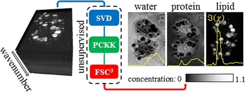
In this work, we report a method to acquire and analyze hyperspectral coherent anti-Stokes Raman scattering (CARS) microscopy images of organic materials and biological samples resulting in an unbiased quantitative chemical analysis. The method employs singular value decomposition on the square root of the CARS intensity, providing an automatic determination of the components above noise, which are retained. Complex CARS susceptibility spectra, which are linear in the chemical composition, are retrieved from the CARS intensity spectra using the causality of the susceptibility by two methods, and their performance is evaluated by comparison with Raman spectra. We use non-negative matrix factorization applied to the imaginary part and the nonresonant real part of the susceptibility with an additional concentration constraint to obtain absolute susceptibility spectra of independently varying chemical components and their absolute concentration. We demonstrate the ability of the method to provide quantitative chemical analysis on known lipid mixtures. We then show the relevance of the method by imaging lipid-rich stem-cell-derived mouse adipocytes as well as differentiated embryonic stem cells with a low density of lipids. We retrieve and visualize the most significant chemical components with spectra given by water, lipid, and proteins segmenting the image into the cell surrounding, lipid droplets, cytosol, and the nucleus, and we reveal the chemical structure of the cells, with details visualized by the projection of the chemical contrast into a few relevant channels.

Coherent anti-Stokes Raman scattering microscopy has emerged in the past decade as a powerful multiphoton microscopy technique for rapid label-free imaging of organic materials and biological samples with submicrometer spatial resolution in three-dimensions and high chemical specificity.^1,2 CARS is a third-order nonlinear process in which molecular vibrations are coherently driven by the interference between two optical fields (pump and Stokes), and the optical field (the pump in two-pulse CARS) is anti-Stokes Raman scattered by the driven vibrations. Owing to the coherence of the driving process, CARS benefits, unlike spontaneous Raman, from the constructive interference of light scattered by spectrally overlapping vibrational modes within the focal volume, enabling fast acquisition at moderate powers compatible with live cell imaging.

Among the various technical implementations of CARS microscopy reported to date, hyperspectral CARS imaging is receiving increasing attention due to its superior chemical specificity over single-frequency CARS. In hyperspectral CARS, a CARS spectrum is measured at each spatial position either by taking a series of spatially resolved images at different vibrational frequencies³ or by acquiring a spectrum at each spatial point following simultaneous excitation of several vibrations.¹ Analyzing the resulting multidimensional data set in order to provide an efficient image visualization and a useful chemical interpretation is nontrivial. Simple approaches to reduce the dimensionality by studying spectra acquired at a few specific positions of the image or by considering images acquired at a few vibrational frequencies fail to make full use of the available information. Moreover, for a quantitative chemical analysis of CARS microspectroscopy images, one has to consider that the quantity which is linear in the chemical composition is the complex third-order susceptibility in the nonlinear process.¹ The CARS intensity is instead proportional to the absolute square of this susceptibility, which contains the interference between the resonant and nonresonant terms resulting in a nontrivial line shape. To overcome this complication, more advanced technical implementations have been developed such as heterodyne coherent anti-Stokes Raman scattering (HCARS),^4,5 which measures amplitude and phase and in turn the complex susceptibility, and stimulated Raman scattering (SRS),⁶⁻⁸ which measures only the imaginary part of the susceptibility. On the other hand, the complex susceptibility can also be determined from the more commonly measured CARS intensity by phase retrieval^9,10 if a spectrum over a sufficiently large spectral range is acquired. Two types of phase-retrieval methods have been discussed recently in the literature, including the modified Kramers–Kronig transform (MKK)¹⁰ and the maximum entropy method (MEM).¹¹ Both methods have been shown to be able to retrieve the complex susceptibility with similar accuracy.¹² They show an error of the retrieved phase of the complex susceptibility, which was partially corrected by subtracting a slowly varying function from the retrieved phase, determined by a procedure which was, however, not well documented. To subsequently represent from the retrieved complex susceptibility a spatially resolved map of spectral components, methods that have been proposed so far in the literature use principal component analysis (PCA)¹³ or hierarchical cluster analysis (HCA)¹⁴ as known from Raman imaging, independent component analysis (ICA) for SRS,¹⁵ classical least-squares (CLS) analysis for CARS,¹⁶ and multivariate curve resolution (MCR) analysis for SRS.⁸ However, although these methods provide a way to sort the spectral information into significant components, they are not able to make an unsupervised decomposition into individual chemical species with quantitative absolute concentration determination, which is ultimately the most meaningful quantitative representation. Among the mentioned methods, MCR can provide a quantitative determination of the chemical composition but needs an initial guess of the spectra¹⁷ and is thus not unsupervised.

Here we present a method of quantitative chemical imaging going from data acquisition using hyperspectral CARS to unsupervised analysis and visualization of the spatially resolved absolute concentrations of chemical components. We use a single source multimodal CARS microscope³ to rapidly acquire hyperspectral CARS images over a large vibrational range from 1200 to 3800 cm^–1. The data are de-noised by singular value decomposition (SVD), and we develop and use two methods for the retrieval of the complex susceptibility based on the causality of the response, where the phase error is corrected as demanded by causality. For the final step, the decomposition into spectra of independently varying chemical components and quantification of their absolute concentrations, we apply a fast variant of non-negative matrix factorization (NMF) with an additional concentration constraint using the imaginary part and the spectrally averaged real part of the susceptibility.

Materials and Methods

CARS Microspectroscopy

CARS hyperspectral images have been acquired on a home-built multimodal laser-scanning microscope based on an inverted Nikon Ti–U with simultaneous acquisition of CARS, two-photon fluorescence (TPF), and second harmonic generation (SHG) using a single 5 fs Ti:Sa broadband (660–970 nm) laser source. A detailed description of the setup can be found in ref (3). In brief, pump and Stokes beams for CARS excitation are given by the laser wavelength ranges of 660–730 nm and 730–900 nm, respectively. We use spectral focusing^18,19 by applying an equal linear chirp to pump and Stokes pulses through glass dispersion. This provides a tunable vibrational excitation covering the 1200–3800 cm^–1 range with a spectral resolution of 10 cm^–1 by varying the time delay between pump and Stokes with a 10 ms step response. The data discussed in this paper were taken with a 20× 0.75 NA dry objective (Nikon CFI Plan Apochromat λ series) and a 0.72 NA dry condenser for signal collection in the forward direction, with a resulting spatial resolution for the material susceptibility (full-width at half-maximum of the coherent point-spread function amplitude) of 0.9 (3.5) μm in the lateral (axial) direction. The CARS signal is discriminated by a pair of Semrock band-pass filters FF01-562/40 for acquisition in the 2400–3800 cm^–1 range, or a Semrock low-pass filter SP01-633RS and a band-pass filter FF01-609/54 for acquisition in the 1200–2500 cm^–1 range, and then detected by a Hamamatsu H7422-40 photomultiplier.

Phase Retrieval

Two methods for the retrieval of the CARS susceptibility in the spectral domain χ̃(ω) were developed and used. They start from the CARS intensity given by I_C(ω) = with the instrument response . The instrument response contains two main effects, the spectrally dependent sensitivity and the finite spectral resolution, limited, for example, by the finite duration of the laser pulses. The instrument response is consequently approximated as the absolute square of the convolution of the susceptibility with a spectral instrument response _s, multiplied with a spectrally dependent transduction coefficient T(ω):

1

_s determines the spectral resolution of the instrument and is assumed to be independent of the center frequency. We do not explicitly consider _s in the following mathematical treatment, such that the retrieved χ̃ will have a spectral resolution limited by _s, which in the present experiments is approximately 20 cm^–1. Separating χ̃ = χ̃_e+ χ̃_v into a nonresonant, frequency-independent real electronic contribution χ̃_e and a complex resonant vibrational contribution χ̃_v, we arrive at

2

To determine T(ω), we use the CARS intensity I_ref(ω) acquired under otherwise identical conditions in a nonresonant medium with susceptibility χ̃_ref (for example, glass for the spectral range of our instrument), yielding T = I_ref/|χ̃_ref|². The CARS ratio is then defined as I̅_C = I_C/I_ref = |χ̃/χ̃_ref|², and we define the normalized susceptibility = χ̃/|χ̃_ref|, which will be used in the following calculations. Making this normalization is an important advantage of the present work, as will be further discussed later. Note also that this simple way of referencing the signal to a known response using glass is an advantage of CARS compared to SRS because SRS is not sensitive to the nonresonant susceptibility. Glass thus provides an ubiquitous calibration standard, typically part of the microscope sample.

Iterative Kramers–Kronig Method (IKK)

In this method, we use the causality of . To do this, we note that from eq 2 we find

3

The inverse Fourier transform of the real part of the susceptibility is related to the susceptibility in time domain χ̅_v(t) = ^–1(_v)

4

where is the Fourier transform operator. The causality of the susceptibility implies that χ̅_v(t) = 0 for negative times, t < 0. We can therefore retrieve χ̅_v by multiplying both terms of eq 4 with the Heaviside function θ(t) and apply a forward Fourier transform,

5

In order to determine _v, we have to know _e and |_v|². Both are determined by iteration for self-consistency. _e is determined from the average value of I̅_C – |_v|² over the spectrum,

6

noting that the spectral average of is zero. The iteration repeats the sequence eq 3 - eq 5 - eq 6 until sufficient convergence is achieved. During the iteration, we can self-consistently determine outside of the measured frequency range. More details on initialization and convergence control of the iteration are given in the Supporting Information. We introduce a Gaussian time filter by replacing θ(t) in eq 5 with θ̃(t) = θ(t) exp (−(t/τ₀)²/2), which suppresses noise beyond the coherence time of the susceptibility and the wrap-around effects in the fast Fourier transform (FFT) algorithm that was used. For the data shown in this work, we used τ₀ = 3 ps given by the experimental spectral resolution.

Phase-Corrected Kramers–Kronig Method (PCKK)

The causality of results in Kramers–Kronig (KK) relationships between the real and imaginary parts of . However, only || is known from a CARS measurement, necessitating the above-described iterative procedure. To alleviate this, one can use the fact that also ln() obeys KK relationships²⁰ and causality. This provides a relationship between (ln()) = ln((I̅_C)^1/2) which we measure, and (ln()), which is the phase ϕ of = ||exp(iϕ). Therefore, no iterative procedure is required, and we can directly retrieve the phase ϕ(ω) by

7

Equation 7 uses the causality principle as in eq 5, but applied to ln() rather than to _v. We note that I̅_C is not measured over an infinite spectral range, such that the values outside of the measured spectral range have to be estimated before applying eq 7. We use here a constant continuation of the measured values, as described in the Supporting Information. This approximation is reasonable for measured ranges with limits in regions without resonances. In order to correct to some extent for the resulting error in the phase, we introduce a rigid phase shift ϕ₀ given by the minimum of ϕ over the measured frequency interval [ω₁,ω_u], such that the corrected phase ϕ_c = ϕ – ϕ₀ is larger or equal than zero over [ω₁,ω_u]. Having retrieved the phase, the real and imaginary part of the susceptibility are determined by

8

The numerical complexity of PCKK is thus given by the calculation of the logarithm and the root, as well as the FFT forward and backward transform. We employ the time-domain filtering described in the IKK method also here, replacing θ(t) with θ̃(t) in eq 7. The time-filtering results in a spectral smoothing reducing the noise and not systematically influencing the phase outside spectral resonances. Noise in the data shifts ϕ₀ to lower values as it is the minimum of ϕ. To suppress this effect, we determine ϕ₀ from ϕ retrieved with a τ₀, which is smaller than the one used to retrieve ϕ to determine ϕ_c. In the data presented here, we used τ₀ = 0.4 ps for ϕ₀ and τ₀ = 3 ps for ϕ_c. We note that a similar field retrieval method (MKK) based on a modified Kramers–Kronig transform was previously reported.¹⁰ In this method, I_ref was not used to normalize I_C, but as negative time component in a phase retrieval similar to eq 7. Using the analytical properties of the method, we found that this is equivalent to a correction of the phase error created by T(ω). However, was then retrieved using = sin(ϕ_c)(I_C)^1/2, which is not corrected for the amplitude factor 1/(T(ω))^1/2, and also not normalized with respect to a known material (see Figure S1 of the Supporting Information for a comparison between the MKK and PCKK methods).

In ref (12), the retrieved phase was corrected by subtracting a spectrally slowly varying baseline. In other previous work using MKK,^16,21 the retrieved spectra are corrected by determining a polynomial baseline and subtracting the baseline on a pixel by pixel basis.

Singular Value Decomposition for Noise Filtering and Spectral Encoding

The compact singular value decomposition is a factorization of a S × P matrix D into

9

In the present application, the P elements are the spatial points of the image, the S elements are the measured spectral points, and we assume P > S. U is a S × S unitary matrix containing a new spectral basis (called the left singular vectors), Σ is a S × S diagonal matrix containing the average contributions (singular values) of the new spectral basis vectors in D, and V^T (transpose of V) is a S × P matrix containing the normalized right singular vectors, which are the spatial distributions in the new spectral basis. Importantly, the new basis is chosen such that the cross-correlation between the new spatial distributions vanishes. The SVD thus finds a new spectral basis with uncorrelated spatial distributions and sorts them according to their average contributions.

Noise Filtering

The noise in I_C is given by the photon shot noise multiplied by the excess noise factor of the photomultiplier used in the detection. The noise is therefore at large photon numbers proportional to (I_C)^1/2, such that I_C/(I_C)^1/2 = (I_C)^1/2 has a intensity independent (also called whitened) Gaussian noise. To remove spectral components which are dominated by this spatially and spectrally uncorrelated noise, we calculate the SVD for the data D, given by (I_C)^1/2 for each point. The singular values of white Gaussian noise are well described by a linear decrease versus index as shown in the Supporting Information Figure S6. Assuming that at least half of the singular vectors are dominated by noise, we can determine this dependence by fitting a linear slope to the singular values with indices larger than S/2. We then classify singular values as being noise-dominated when they are less than a factor (2)^1/2 larger than the fit (i.e., when their root-mean-square (RMS) signal is estimated to be less than the RMS noise), resulting in an index cutoff of i_max. We remove these noise-dominated components by setting their singular values to zero, resulting in the matrix Σ_nf, and the noise-filtered data

10

The noise-filtered CARS data is then used for the field retrieval algorithms. In previous work, this filtering was done directly in I_C, which is less effective in separating the signal from the noise, as shown in Figure 3, and the filter cutoff was determined using a subjective analysis of the spatial distributions of the singular components.¹⁶

Figure 3.

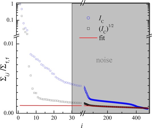
Singular values of the SVD noise-filtering procedure. Squares and circles show singular values of (I_C)^1/2 and I_C, respectively, and the red line is a linear fit to the singular values of (I_C)^1/2 for i > 240. The gray area indicates the values set to zero for noise filtering.

Spectral Encoding

The number of independent channels recognizable in an image is limited to three, given by the number of color channels in human vision. However, the number of spectral channels in vibrational spectra is typically significantly larger than three, so that we need a method to distill the most significant information of an image into these three channels. SVD is suited for this, as it calculates a new basis of ordered importance, allowing us to show the most important three singular vectors which are capturing the largest part of information, typically creating more than 90% of the total variance in the data.

Blind Factorization into Susceptibilities and Concentrations of Chemical Components

We assume that the CARS susceptibility _p measured at any voxel p of the image is given by the weighted sum of the susceptibilities ^{k} of chemical components numbered by k with non-negative relative volume concentrations c_p^{k}, such that

11

where K is the number of relevant components. Furthermore, each component has a susceptibility with a non-negative imaginary part, ≥ 0, and a positive nonresonant background, _e. The resonant contribution to , which is , is fully determined by = and thus does not contain additional information. It is therefore adequate to use non-negative matrix factorization (NMF) of over the measured spectral points and an additional point for _e. We determine the value χ̂_e of this additional point by the spectral average of weighted with the root of the number of points to provide the same RMS error as each spectral point of ,

12

The P × (S + 1) matrix of data D = {{},χ̂_ep} is then factorized into the non-negative P × K matrix of concentrations C = {c_p^{k}} and a non-negative (S + 1) × K matrix of spectra S = {{},χ̂_e} of the components, such that

13

where E is the residual of Frobenius norm ||E||, which is minimized by the NMF. We employ the iterative fast block principal pivoting algorithm²² to perform this minimization. NMF determines the product of concentrations and spectra, with an arbitrary scaling between them, such that the resulting concentrations, as well as the spectra, are in arbitrary units. If we assume that the voxel volume is completely filled with components which are measured in CARS, we can use the physical constraint that the sum of the volume concentrations at each voxel is equal to one, which determines the scaling and thus determines the factorization into susceptibilities and concentrations of the chemical components (FSC³) in absolute units. To implement this constraint, we modified the algorithm in ref (22) by adding to each iteration step (which consists of a minimization of ||E|| over S, followed by a minimization of ||E|| over C) a minimization of the concentration error |E_C|, where E_C = {1–∑_k = 1^Kc_p}, over a position-independent scaling of the concentration of each component, using the same minimization algorithm.

Results and Discussion

Phase Retrieval of Simulated Spectra

To verify the validity of the phase-retrieval methods IKK and PCKK and to compare their performance with the methods MKK and MEM reported in the literature, we first use simulated spectra exactly adhering to the assumptions of the methods, as discussed in the Supporting Information Figure S2. In essence, all methods lead to an acceptable result for this simulation, with the MEM and PCKK showing the smallest errors. The fastest method is PCKK because it uses only a double Fourier transform operation.

Phase Retrieval of Measured Spectra

We apply now the phase retrieval to data measured with our single-source CARS microscope. The spectra of I̅_C for bulk PS and GTO samples are shown in Figure 1 (a,c). The sample preparation is described in the Supporting Information. The CARS intensity spectra of the samples and of glass have been acquired in the spectral ranges of 1200–2400 and 2200–3900 cm^–1 using appropriate filters and dispersion settings,³ and I̅_C was generated from this data in the range of 1200–3900 cm^–1 for the PCKK, IKK, and MEM methods. For the MKK method, which uses I_C, was retrieved separately in the two spectral ranges. The retrieved values are shown in Figure 1 (b,d), together with of the MKK method in arbitrary units. All major features observed in the Raman spectra (details of the confocal Raman microspectrometer can be found in the Supporting Information) acquired on the same samples (dashed lines) are reproduced in the retrieved , including the weak resonances at (2980, 3003, 3164, 3203) in the PS spectrum and the peak at 1744 cm^–1 from the C=O stretch of the ester bonds between glycerol and the oleic acid²³ in the GTO spectrum. The IKK and MEM methods produce almost identical imaginary parts of the susceptibility, while the MKK result differs mainly because of the only partially corrected transduction T(ω). , retrieved by IKK, MEM, and MKK, shows a negative offset. In the PCKK method, which includes phase correction, a positive is obtained. We note that correcting , as done in ref (16), instead of correcting the phase, leads according to eq 8 to an inconsistency of retrieved and measured I̅_C. In the inset of Figure 1, the RMS error in the iterative method is shown as a function of the iteration steps (see the Supporting Information for details). The minimum RMS error is obtained within 20 iterations. A further example, the spectrum of a lipid droplet in a 3T3L1-derived adipocyte, is shown in Supporting Information Figure S7.

Figure 1.

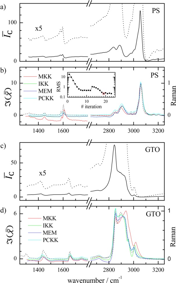
CARS intensity ratio I̅_C measured on bulk samples of PS in (a) and GTO in (c) and the corresponding retrieved in (b,d) for different methods as labeled. Normalized Raman spectra measured on the same samples are shown as dashed lines. The RMS error in I̅_C of the IKK method versus iteration number is shown in the inset of (b).

Determination of Spectra and Absolute Concentrations of a Lipid Mixture Using FSC³

Hyperspectral CARS images and Raman spectra of the octanoic acid/α-linolenic acid mixtures were acquired in the frequency region of 2400–3800 cm^–1. The sample preparation is described in the Supporting Information. The CARS images cover an area of 10 × 10 μm², and a spectral step of 3 cm^–1 size has been used. After SVD de-noising with i_max = 20, has been retrieved using PCKK. FSC³ with K = 2 was then applied to the ensemble of (Raman) spectra of the different mixtures, resulting in the spectra and concentrations shown in Figure 2a,b, respectively. The FSC³ spectra quantitatively reproduce the spectra of the pure substances with deviations in the few percent range, showing that FSC³ is able to determine the component spectra without supervision. The resulting absolute concentrations of the FSC³ components are shown in the inset versus the nominal concentration, showing an error of a few percent. Interestingly, the performance of FSC³ on Raman and CARS data is similar, implying that hyperspectral CARS can provide similar chemical specificity as Raman. We note that the two components that were used differ only by 24% in their Raman spectra (given by the norm of the difference). Concentrations of components with larger differences are expected to be retrieved with a smaller error. We have compared the performance of the MCR factorization method used in ref (8) with FSC³ (details given in Figure S8 of the Supporting Information). We find that apart from being about 2 orders of magnitude slower, the MCR method fails to deterministically reproduce the spectra and concentration of the chemical components if a random initial guess for the spectra is used, as used in FSC³ and required for an unsupervised and unbiased determination of the absolute chemical composition of the sample.

Figure 2.

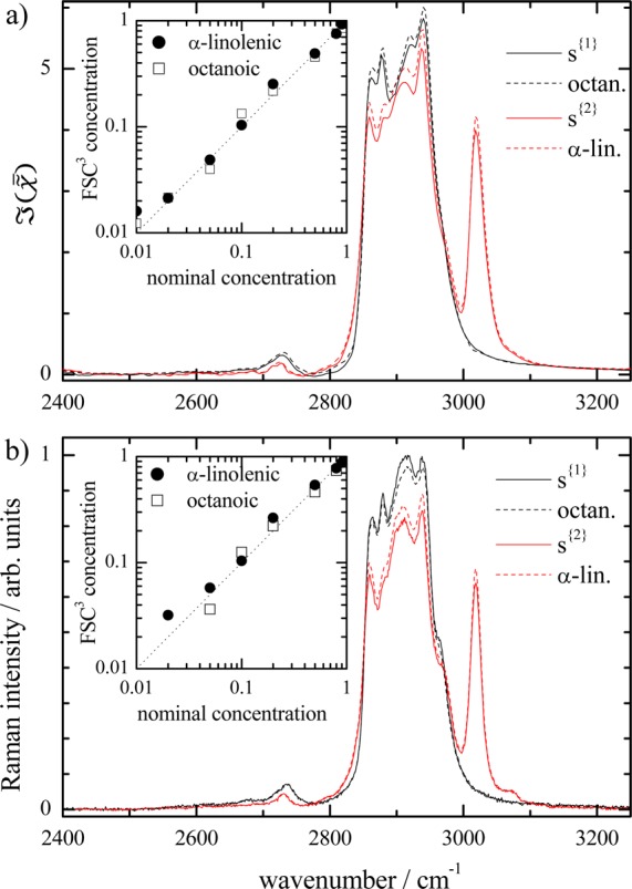
a) FSC³ spectra s^{k} (solid lines) of mixtures of octanoic and α-linolenic acid, compared with the spectra of the pure compounds (dashed lines). Inset: FSC³ concentrations (v/v) c^{k} versus nominal concentration. (b) as (a) for Raman spectra.

Analysis of Hyperspectral CARS Images of Cells

Hyperspectral CARS images of fixed 3T3L1-derived adipocytes were acquired with a pixel size of 0.3 × 0.3 μm² and 3 cm^–1 spectral steps in the two frequency ranges, 1200–2400 and 2200–3900 cm^–1. The sample preparation is described in the Supporting Information. To show the difference between using (I_C)^1/2 or I_C in the SVD noise filtering, we show in Figure 3 the singular values Σ_i,i for both cases, normalized to the respective largest value Σ_1,1. The singular values of (I_C)^1/2 are decaying faster, and they show a linear decay with index for the higher indices, as expected for white Gaussian noise. The linear fit to the upper half of the values (i > 240) and the resulting cutoff (i_max = 30) is also shown. The singular values of I_C instead do not show the linear behavior and are not suited for the unsupervised noise filtering. Using the noise-filtered I̅_C, we retrieve with PCKK. For visualization, we use SVD on and show images of the first five singular components in Figure 4. The first component is dominant outside the cells and can be associated to water, in agreement with the spectrum having a dominant band around 3350 cm^–1 that is related to the O–H stretch modes. The second component shows the lipid droplets in the cells with a spectrum peaked at 2850 cm^–1, corresponding to the CH₂ stretching mode. The third component is present in the other regions of the cell, including the cytosol, nuclear membrane, and nucleoli. Its spectrum shows a peak around 2930 cm^–1 which is typical for proteins/nucleic acids.⁸ The fourth component relates to inhomogeneities in the chemical composition of the lipid droplets. The fifth component is a modification of the water spectrum and fluctuates within the cytosol and the nucleus. SVD decomposition results for IKK-derived are shown in the Supporting Information Figure S9.

Figure 4.

Results of a SVD on hyperspectral images of measured on 3T3L1-derived adipocytes in the 2400–3800 cm^–1 range and retrieved with PCKK. Top: Spatial distribution of ΣV^T of the first five singular components on a linear grayscale with black (white) corresponding to the minimum (maximum) value, respectively. Scale bar indicates 5 μm. Bottom: two images with color encodings labeled by the singular component number after each color letter. Graphs: (a) first five singular spectra, vertically displaced for clarity, (b) singular values, (c) spectra at the positions indicated by the symbols in the R1G2B3 image.

The spatial distribution of up to three singular components can be shown in color images. This is illustrated in Figure 4 which shows a RGB image encoding the first component as red, the second as green, and the third as blue. Using alternative encodings can vary the contrast, as shown in the RGB image created with the fourth, fifth, and sixth component as red, green, and blue channels, respectively.

In the SVD images of (I_C)^1/2, shown in the Supporting Information Figure S10, the lipid droplets are surrounded by a thin layer of a different component. This is a result of the interference between χ̃_e and χ̃_v in (I_C)^1/2. In the corresponding images of (see Figure 4 for PCKK and Supporting Information Figure S9 for IKK), the lipid droplets are homogeneous in color, indicating a homogeneity in the chemical composition.

The SVD spectra of do not correspond to individual chemical components but rather to differences between chemical components fluctuating independently. The SVD analysis helps to determine regions of the samples which present the same color and that can be identified as a single substance. Once a substance is identified, one can rotate the basis by manually defining regions which are assumed to be pure substances, as detailed in the Supporting Information Figure S11. However, this is a subjective procedure and does not apply the physical constraints which are used in the FSC³ method of blind factorization into susceptibilities and concentrations of chemical components.

The results of FSC³ on are shown in Figure 5 for K = 4 chemical components. Both the spatial distribution of the components concentration and their spectra can be attributed to expected chemical components. Component 1 has the largest volume fraction (53%) within the image, and both the spectrum and spatial distribution are consistent with its attribution to water. Component 4 has a volume fraction of 9%, has a spectrum similar to GTO (compare Figure 1), and is highly concentrated in the droplet structures. This shows that these structures are lipid droplets. Component 2 has a volume fraction of 26%, is spatially located in the cytosolic regions and in the nucleus, and has a spectrum peaked around 2930 cm^–1. This component is attributed to proteins and nucleic acids .⁸ Interestingly, it shows not only the CH₃ resonance around 2930 cm^–1 but also comes with a water component which has a slightly modified spectrum compared to the bulk water spectrum of component 1. From the comparison between the area of the water peak in components 1 and 2, we can estimate a 57% relative volume fraction of water in this component. This can be interpreted as the volume of a solvation layer around the proteins and nucleic acids. Assuming a 1 nm thick solvation layer,²⁴ the relative volume fraction is expected for core sizes of 4(6) nm for a cylindrical (spherical) geometry, respectively. These sizes are within a factor of 2, consistent with protein/nucleic acid sizes, supporting the attribution of the modified water component to a solvation layer. Finally, component 3 is mostly present at the membrane of the lipid droplets, characterized by a small peak at ∼2750 cm^–1 and a deformed water spectrum, but it has a relative concentration much smaller than the other substances. This is the weakest component and is attributed to a mixture of components of lower concentration not captured by the other components. By increasing the number of components, K, the spectra of component 2 and 4 split into more components with slightly different water/protein/lipid spectral features. This is expected because there are many different lipids/proteins and solvation layers in the complex cell machinery. A color image encoding the concentrations of components 1 in blue, 4 in green, and 2 in red gives a good rendering of the chemical structure, as shown in Figure 5. The error of the factorization is quantified by the relative spectral error, E_s = (P∑_s = 1^SE_s,p)^1/2/ ||D||, and is shown in Figure 5. The maximum relative error is 31% and is localized at large lipid droplets. The average spectral error is 3.5%. The relative concentration error E_C is also shown in Figure 5 and has a maximum of about 25%. Distortions of the excitation fields by the spatial refractive index structure lead to a modulation of the CARS intensity and thus the retrieved concentration. Furthermore, component spectra might change if chemical substances are interacting with each other, which is not captured by the factorization into independent components. The spatial distribution of E_C shown in Figure 5 indicates that E_C is dominated by the refractive index structure, having minima at the edges and maxima at the center of the droplets. The spatial distribution of E_S gives complementary information to E_C, indicating regions which contain spectral features and thus chemical compositions which are not captured by the FSC³ components. The sensitivity of FSC³ can be enhanced by selecting regions of interest in the spatial and spectral domain. To resolve chemical differences between cytosol, nucleus, and nucleoli, we have analyzed only the corresponding spatial region, and we have reduced the spectra range to 2500–3100 cm^–1 to reject the contribution of the water spectrum. The result (bottom row of Figure 5) reveals that nucleoli and the nuclear membrane contain mostly proteins/nucleic acids (component 2), while the cell cytosol shows a mixed protein–lipid composition (component 4). Water (component 1) is the dominant component of the nucleoplasm.

Figure 5.

Results of FSC³ with K = 4 on described in Figure 4. Top: spatial distributions of the volume concentration C. Grayscale ranges from 0 (black) to 1.1 (white). The corresponding component spectra are displayed in (a) together with the spectrally averaged (dashed lines). Middle: color concentration image using the first component as blue, the second as red, and the fourth as green, scaled to saturate at the concentration maximum. The spatial distribution of the concentration error E_C is shown on a grayscale from −0.28 to 0.16, and the spatial distribution of the spectral error E_S is shown on a grayscale from 0.005 to 0.31. Bottom: Results of FSC³ using a restricted spatial range as shown and spectral range 2500–3100 cm^–1. Grayscale ranges from 0 (black) to 0.74 (white). Corresponding component spectra are displayed in (b). Scale bars indicate 5 μm.

The inclusion of the nonresonant susceptibility in the factorization, afforded by the use of CARS as opposed to SRS, is specifically important for samples containing components without significant vibrational resonances in the measured spectral range. This is the case for water in the characteristic region. As an example, we have performed FSC³ of the same cells as Figure 5 in the characteristic region, as discussed in the Supporting Information Figure S12. We find that the resulting concentration error E_C is in the order of 100% when not including the nonresonant susceptibility. The FSC³ analysis is also suited for samples with a weak resonant susceptibility. As an example of this case, we have imaged differentiated mouse embryonic stem cells (ESc), as discussed in the Supporting Information Figure S15.

Summary

In summary, we have demonstrated a new method which we call FSC³ to quantitatively analyze and visualize effectively the spectral information contained in hyperspectral CARS microscopy images. The method employs de-noising by singular value decomposition on whitened CARS intensity data with an autonomous identification of noise components. The subsequent phase retrieval is done using a fast noniterative algorithm (PCKK) based on the causality of the response, yielding the susceptibility, which is linear in the concentration of the chemical components. We then use the physical constraint of positive concentrations, the positive imaginary part of the susceptibility as well as the positive nonresonant real susceptibility, to determine the susceptibilities and absolute concentrations of individual chemical components from the hyperspectral images. The validity and effectiveness of the PCKK method in comparison to other methods in the literature is demonstrated using simulated spectra as well as measured CARS and Raman spectra of polystyrene and lipids. The ability of FSC³ to quantify absolute concentrations is demonstrated using lipid mixtures. Finally, the efficacy of the method to provide an unsupervised analysis and visualization of the spatially resolved absolute concentrations of chemical components is shown in adipocytes and differentiated mouse embryonic stem cells. In conclusion, FSC³ can be used in a wide range of applications requiring fast and quantitative volumetric chemical imaging, from live cell microscopy to material science applications, providing an unsupervised technique to identify unknown chemical differences within and between samples.

Supporting Information Available

Additional information as noted in the text. This material is available free of charge via the Internet at http://pubs.acs.org/.

The authors declare no competing financial interest.

References

- Muller M.; Zumbusch A. ChemPhysChem 2007, 8, 2156–2170. [DOI] [PubMed] [Google Scholar]
- Pezacki J. P.; Blake J. A.; Danielson D. C.; Kennedy D. C.; Lyn R. K.; Singaravelu R. Nat. Chem. Biol. 2011, 7, 137–145. [DOI] [PMC free article] [PubMed] [Google Scholar]
- Pope I.; Langbein W.; Watson P.; Borri P. Opt. Express 2013, 21, 7096–7106. [DOI] [PubMed] [Google Scholar]
- Potma E. O.; Evans C. L.; Xie X. S. Opt. Lett. 2006, 31, 241–243. [DOI] [PubMed] [Google Scholar]
- Jurna M.; Korterik J. P.; Otto C.; Herek J. L.; Offerhaus H. L. Phys. Rev. Lett. 2009, 103, 043905. [DOI] [PubMed] [Google Scholar]
- Freudiger C. W.; Min W.; Saar B. G.; Lu S.; Holtom G. R.; He C.; Tsai J. C.; Kang J. X.; Xie X. S. Science 2008, 322, 1857. [DOI] [PMC free article] [PubMed] [Google Scholar]
- Ozeki Y.; Dake F.; Kajiyama S.; Fukui K.; Itoh K. Opt. Express 2009, 17, 3651–3658. [DOI] [PubMed] [Google Scholar]
- Zhang D.; Wang P.; Slipchenko M. N.; Ben-Amotz D.; Weiner A. M.; Cheng J.-X. Anal. Chem. 2013, 85, 98–106. [DOI] [PMC free article] [PubMed] [Google Scholar]
- Rinia H. A.; Bonn M.; Müller M.; Vartiainen E. M. ChemPhysChem 2007, 8, 279–287. [DOI] [PubMed] [Google Scholar]
- Liu Y.; Lee Y. J.; Cicerone M. T. Opt. Lett. 2009, 34, 1363. [DOI] [PMC free article] [PubMed] [Google Scholar]
- Vartiainen E. M.; Rinia H. A.; Müller M.; Bonn M. Opt. Express 2006, 14, 3622–3630. [DOI] [PubMed] [Google Scholar]
- Cicerone M. T.; Aamer K. A.; Lee Y. J.; Vartiainen E. J. Raman Spectrosc. 2012, 43, 637–643. [Google Scholar]
- Miljkovic M.; Chernenko T.; Romeo M. J.; Bird B.; Matthaus C.; Diem M. Analyst 2010, 135, 2002–2013. [DOI] [PubMed] [Google Scholar]
- van Manen H.-J.; Kraan Y. M.; Roos D.; Otto C. Proc. Natl. Acad. Sci. U.S.A. 2005, 102, 10159–10164. [DOI] [PMC free article] [PubMed] [Google Scholar]
- Ozeki Y.; Umemura W.; Otsuka Y.; Satoh S.; Hashimoto H.; Sumimura K.; Nishizawa N.; Fukui K.; Itoh K. Nat. Photonics 2012, 6, 845–851. [Google Scholar]
- Lee Y. J.; Moon D.; Migler K. B.; Cicerone M. T. Anal. Chem. 2011, 83, 2733–2739. [DOI] [PubMed] [Google Scholar]
- Huang C.-K.; Ando M.; Hamaguchi H.-O.; Shigeto S. Anal. Chem. 2012, 84, 5661–5668. [DOI] [PubMed] [Google Scholar]
- Hellerer T.; Enejder A. M.; Zumbusch A. Appl. Phys. Lett. 2004, 85, 25–27. [Google Scholar]
- Rocha-Mendoza I.; Langbein W.; Borri P. Appl. Phys. Lett. 2008, 93, 201103. [Google Scholar]
- Smith D. Y. J. Opt. Soc. Am. 1977, 67, 570–571. [Google Scholar]
- Parekh S. H.; Lee Y. J.; Aamer K. A.; Cicerone M. T. Biophys. J. 2010, 99, 2695–2704. [DOI] [PMC free article] [PubMed] [Google Scholar]
- Kim J.; Park H. SIAM J. Sci. Comput. 2011, 33, 3261–3281. [Google Scholar]
- Di Napoli C.; Masia F.; Pope I.; Otto C.; Langbein W.; Borri P. J. Biophotonics 2012, 10.1002/jbio.201200197. [DOI] [PubMed] [Google Scholar]
- Ebbinghaus S.; Kim S. J.; Heyden M.; Yu X.; Heugen U.; Gruebele M.; Leitner D. M.; Havenith M. Proc. Natl. Acad. Sci. U.S.A. 2007, 104, 20749–20752. [DOI] [PMC free article] [PubMed] [Google Scholar]
Associated Data
This section collects any data citations, data availability statements, or supplementary materials included in this article.