Force Field for Peptides and Proteins based on the Classical Drude Oscillator

Abstract

Presented is a polarizable force field based on a classical Drude oscillator framework, currently implemented in the programs CHARMM and NAMD, for modeling and molecular dynamics (MD) simulation studies of peptides and proteins. Building upon parameters for model compounds representative of the functional groups in proteins, the development of the force field focused on the optimization of the parameters for the polypeptide backbone and the connectivity between the backbone and side chains. Optimization of the backbone electrostatic parameters targeted quantum mechanical conformational energies, interactions with water, molecular dipole moments and polarizabilities and experimental condensed phase data for short polypeptides such as (Ala)₅. Additional optimization of the backbone φ, ψ conformational preferences included adjustments of the tabulated two-dimensional spline function through the CMAP term. Validation of the model included simulations of a collection of peptides and proteins. This 1^st generation polarizable model is shown to maintain the folded state of the studied systems on the 100 ns timescale in explicit solvent MD simulations. The Drude model typically yields larger RMS differences as compared to the additive CHARMM36 force field (C36) and shows additional flexibility as compared to the additive model. Comparison with NMR chemical shift data shows a small degradation of the polarizable model with respect to the additive, though the level of agreement may be considered satisfactory, while for residues shown to have significantly underestimated S² order parameters in the additive model, improvements are calculated with the polarizable model. Analysis of dipole moments associated with the peptide backbone and tryptophan side chains show the Drude model to have significantly larger values than those present in C36, with the dipole moments of the peptide backbone enhanced to a greater extent in sheets versus helices and the dipoles of individual moieties observed to undergo significant variations during the MD simulations. Although there are still some limitations, the presented model, termed Drude-2013, is anticipated to yield a molecular picture of peptide and protein structure and function that will be of increased physical validity and internal consistency in a computationally accessible fashion.

INTRODUCTION

Empirical force field studies of peptides and proteins are widely used to understand the structural and dynamical properties of this biologically important class of molecules and relate them to their chemical functions. To date, these studies have largely been based on non-polarizable, additive force fields where the partial atomic charges of the system are fixed effective values accounting for induced electronic polarization in a mean-field manner, with the mostly widely used models including AMBER,^{1, 2} CHARMM,^3–5 GROMOS⁶ and OPLS,^{7, 8} among others.^{9, 10} Efforts to go beyond the additive approximation by incorporating an explicit treatment of electronic polarization have been ongoing for close to 30 years.^11–13 Already in 1976, Warshel and Levitt presented a polarizable model of lysozyme in which polarization was incorporated via interacting induced point-dipoles.¹¹ Subsequent work over the following decades involved a range of developments that were critical to allow computationally efficient molecular dynamics (MD) simulations of solvated biological macromolecules based on polarizable models.^14–18 Such models, in which the electronic properties vary as a function of environment, are anticipated to yield a more physically realistic and consistent model, which would hopefully be more capable of reproducing a wide range of experimentally quantifiable observables accurately.

Towards the goal of a polarizable protein force field (FF) amenable to MD simulations, Berne, Friesner and coworkers introduced both induced dipole and fluctuating charge polarizable models,¹⁹ as well as combinations thereof,^{20, 21} reporting gas phase protein simulations in 2002,²² followed by a simulation in explicit solvent in 2005.^{23, 24} Patel and Brooks presented explicit solvent simulations of proteins in 2004 using a polarizable model based on a dynamically-fluctuating charge model.^{25, 26} AMEOBA, which models the molecular charge distribution using a multipole representation along with induced point dipoles, was originally reported in 2002²⁷ and has been applied for studies of ligand binding to proteins.^28–32 While polarizable MD simulations using these, as well as other models,^{33, 34} have been presented they are typically short in duration, being a few nanoseconds or less, such that the models have yet to be rigorously evaluated as well as used in application studies. A recent exception is a study on lysozyme using the fluctuating charge model implemented in CHARMM,³⁵ where simulations of up to 14 ns displayed RMS differences larger than those from the additive CHARMM22 force field.³ More recently, an updated AMEOBA force field for proteins has been presented.³⁶ The model was optimized targeting both quantum mechanical and experimental data on model compounds and small peptides and used for simulations of a collection of small proteins for 30 ns. Thus, in practice it has clearly been a challenge to bridge the gap from the construction of a physically-motivated polarizable force field for proteins at the conceptual level, and its implementation into a computationally efficient form at the practical level in order to allow one to undertake MD simulations studies for a range of systems and evaluate the robustness and accuracy of the model.

Development of the Drude polarizable force field in our laboratories has been ongoing since 2000.³⁷ Those efforts have lead to the development of water models^37–39 and parameters for a collection of small molecules representative of the functional groups in proteins, nucleic acids, lipids and carbohydrates,^40–48 as well as for ions.^{49, 50} In addition, MD simulation studies of a DNA duplex in solution with counterions⁵¹ and of a Dipalmitoylphosphatidylcholine (DPPC) bilayer and monolayer were reported.⁵² While those studies were based on early models aimed at illustrating specific aspects of induced polarization, they were not based on optimized force field parameters suitable for a wide range of systems. More recently, we have completed refined models for DPPC⁵³ and acyclic polyalcohols.⁵⁴ Thus, progress is being made in extending the Drude polarizable force field from small molecules to biologically relevant macromolecular systems. In the present work we extend those efforts to a polypeptide force field applicable for MD simulation studies of peptides and proteins. Emphasis is placed on optimization of the polypeptide backbone parameters and the connectivity between the backbone and the side chains, whose parameters were obtained from our previous publications with additional adjustments as outlined below. The final model, which will be named Drude-2013, but is referred to as Drude-3 in the present manuscript, is then applied to MD simulations of a collection of peptides and proteins to assess the validity and overall accuracy of the model. The results show that the model yields structural properties, including sampling of backbone and side chain conformations in agreement with experiment at a level similar to that obtained with state-of-the-art additive force fields. We note that the range of proteins studied and the time scales of the present simulations are not adequate to fully probe the ability of the model to reproduce a wide range experimental observables as has been done over time with the additive models,^55–63 such that future improvements in the model are anticipated.

Classical Drude Oscillator Force Field

Explicit polarization in the classical Drude oscillator implementation (also referred to as a Shell or Charge-On-Spring (COS) model^{64, 65}) is based on attaching a charged auxiliary particle with a harmonic spring to the nucleus or atomic core of the parent atom (Figure 1a). The classical Drude originated from the quantum mechanical (QM) Drude model used to treat dispersion,^{66, 67} and has been subsequently used for ionic crystals, simple liquids, water, ions and in QM/MM calculations.¹⁷ In the classical Drude model, the induced atomic dipole, μ, in the present of an electric field, E, is

Figure 1.

Example of the Drude oscillator model in the context of a carbonyl (C=O) group. A) The carbon and oxygen atoms shown as spheres with the atomic core (or nucleus) and the Drude particle, with the associated partial atomic charges for the nucleic, q_C and q_O for carbon and oxygen, respectively, and q_D for the Drude particles, where the value of q_D varies for the different atom types. B) Carbonyl group in the context of a peptide bond showing the approximate positions of the line pairs and the tensor components A11 (red), A22 (green) and A33 (blue) that define the anisotropic atomic polarizability on the oxygen atom. C) Schematic of the orientation of the Drude particles in a diatomic relative to the atomic centers with the electric field, E, parallel and perpendicular to the covalent bond.

$$\mathbf{\mu }=\frac{q_D^2\mathbf{E}}{k_D}.$$ Eq. 1

such that the atomic polarizability, α, is equivalent to the Drude charge, q_D, divided by the force constant on the harmonic spring, k_D,

$$\alpha =\frac{q_D^2}{k_D}.$$ Eq. 2

In practice, the unperturbed static partial atomic charge of the atom, q, is distributed between the parent atom and the virtual Drude particle.

For the sake of simplicity, the current implementation of the classical Drude model introduces atomic polarizabilities only to non-hydrogen atoms. However, this is adequate to accurately reproduce molecular polarizabilties, as seen in a number of published studies.^{41, 42, 47} In the case of hydrogen bond acceptors it has been shown that inclusion of anisotropic atomic polarizability improves non-bond interactions involving acceptors as a function of orientation, especially in the case of interactions with ions.⁴⁴ Anisotropic atomic polarization is defined as the isotropic polarizability times a tensor A, with trace = 3 (Figure 1b). A is diagonal in a local reference frame defined by the vector, A11, between the atom on which anisotropic polarizability is being assigned and a covalently bound atom or, more generally any particle, such as a lone pair. The third and fourth atoms, or particles, define the A22 vector, with the A33 vector being orthogonal to A11 and A22. As the trace of A is set to 3, only the values of A11 and A22 need to be set, such that A33 = 3 – A11 – A22. For example, the specification in the residue-topology-file (RTF) within the CHARMM syntax in the case of the peptide backbone carbonyl O (Figure 1B), is “ANISOTROPY O C CA N A11 0.82322 A22 1.14332,” where the anisotropic polarizability is on the O, the A11 vector is along the C=O bond and the A22 vector is along the CA-N direction. To further facilitate the ability of the model to treat non-bond interactions involving acceptors, virtual particles representative of lone pairs are included in the model.⁴⁴ In the case of the carbonyl O, this involves two LP sites (Figure 1b), whose positions were optimized to improve the interactions with water as a function of orientation.

An important feature in a polarizable force field is the ability of the induced atomic dipoles to interact with each other within a molecule to yield the correct molecular polarizability tensor.^68–70 Traditionally, in additive force fields nonbond interactions between atoms covalently bound to each other (1,2 pairs) or the terminal atoms on a valence angle (1,3 pairs) are ignored while nonbond interactions between the terminal atoms of dihedral angles (1,4 pairs) and beyond are treated explicitly, with 1,4 pair interactions being scaled in some force fields.^{1, 8} However, with a polarizable force field it is possible for all induced atomic dipoles to interact with each other, including 1,2 and 1,3 pairs, as a means to obtain the correct molecular polarization response. An example is the case of diatomic, as shown in Figure 1c. With the diatomic when the electric field is parallel to the bond between the atoms the atomic dipoles interact favorably while when the field is perpendicular to the bond the atomic dipoles interact unfavorably. It is these differences that yield a non-trivial anisotropic molecular polarizability tensor, which in the case of the diatomic will be larger parallel to the bond as compared to perpendicular to the bond. While it is useful to include these interactions in the polarizable force field, their spatial separation is such that the Coulombic approximation fails, disallowing use of point charges for the 1,2 and 1,3 interactions. To overcome this, the electrostatic shielding treatment proposed by Thole is applied⁶⁹, in which the coulomb interactions between charges i and j are modulated by a factor, S_ij, as shown in equation 3

$$S_{ij}\left(r_{ij}\right)=1-\left(1+\frac{\left(a_i+a_j\right)r_{ij}}{2{\left({\alpha }_i{\alpha }_j\right)}^{1/6}}\right)e^{\frac{-\left(a_i+a_j\right)r_{ij}}{2{\left({\alpha }_i{\alpha }_j\right)}^{1/6}}}.$$ Eq. 3

where r_ij is the distance between the atoms, α_i and α_j are the respective atomic polarizabilities, and a_i and a_j are the atom-based Thole parameters that dictate the extent of the scaling between specific atom types. The use of atom-based Thole parameters has been shown to yield improvements in the treatment of the orientation of molecular polarizabilities.⁴¹ In addition, the use of Thole screening has been extended to nonbond atom pairs.⁴⁹ This extension was motivated by the need to fine tune interactions involving divalent ions, but the approach is general and may be applied to any atom pair.

When performing minimization and MD studies using a polarizable model it is necessary, in principle, to perform a self-consistent field (SCF) calculation based on the Born-Oppenheimer Approximation. This assumes that the electronic degrees of freedom relax for each position of the atomic nucleic. With the Drude model, this implies that the Drude particles relax in the electric field for each (fixed) nuclear configuration of the system. This requirement may be satisfied by performing an energy minimization of the Drude particles while the atomic nuclei positions are kept at a fixed position. However, this approach is computational demanding, making it inappropriate for MD simulations. To overcome this the electronic degrees of freedom are treated as classical dynamic variables in the MD simulation assuming an extended Lagrangian approach.^71–73 With the Drude model, this involves ascribing a mass to the Drude particles, which is taken from the parent atom and is typically 0.4 AMU. The extended Lagrangian procedure then allows the Drude particle to propagate classically during the simulation. A dual-thermostat Nose-Hoover algorithm based on the Velocity Verlet integrator was developed⁷⁴ in which the Drude particles are cooled to a very low temperature (near 0 K) during the MD simulation, thereby imposing the electronic degrees of freedom to approach the adiabatic SCF limit. Alternate dual thermostating approaches may be applied, notably based on Langevin dynamics, as has been implemented in the program NAMD.⁷⁵

An issue when performing MD simulations using a polarizable force field is the potential for polarization catastrophe. This may occur when, for example, a positively charged ion approaches to close to an atom, leading the negatively charged Drude particle to become overpolarized, yielding unphysical infinite energies and instabilities. To avoid this issue, two approaches have been implemented. The first involves a “hyperpolarization” term where higher order anharmonic terms are added to the bond between the atomic core and the Drude particle.⁴⁹ Equation 4 shows the form of the hyperpolarization term

$$E_{\mathit{hyp}}=\sum K_{\mathit{hyp}}{\left(R-R_o\right)}^n$$ Eq. 4

where R is the distance between the nucleus and the Drude particle, n is the order of the term, typically 4 or 6, K_hyp is the force constant and R_o defines the distance at which the term starts to impact the Drude particle, typically 0.2 Å, such that the normal trajectory of the Drude is not impacted by the higher order term. More recently, a Drude reflective “hard wall” term has been added to more rigorously avoid polarization catastrophe.⁵³ This term involves reversing the relative velocities along the Drude particle-parent atom nucleus bond and scaling them accordingly to the temperature of the Drude bond whenever the Drude-parent atom bond length exceeds a specified distance, again typically 0.2 Å. In addition the relative displacement with respect to the specified distance is reversed and scaled according to the new velocities on the Drude particle to assure that the location of the Drude is within the specified distance. In practical experience, the reflective hardwall term represents a more robust method to avoid polarization catastrophe as compare to the hyperpolarization terms and is now the recommended approach to be used on all MD simulations using the Drude polarizable force field.

Concerning the computational costs of the Drude implementation, as the model simply involves additional charged particles the overhead is associated directly with the number of Drude particles. Thus, limiting the use of Drude particles to only non-hydrogen atoms limits the number of additional particles such that the increased computational cost is a factor of 1.6 to 2.0.⁷⁵ However, for many molecular systems it is possible to use an integration time step of 2 fs with an additive force field, while the high frequency motions of the Drude particles limit the integration time step to 1 fs for the majority of systems, though a smaller time step may be required for highly ionic systems. In the present study an integration time step of 1 fs was used, unless noted, such that the additional computational cost compared to the additive protein MD simulations is approximately a factor of 4.

METHODS

Quantum Mechanical Calculations

Quantum mechanical (QM) calculations used the programs Gaussian09⁷⁶ and Q-CHEM.^{77, 78} Energy minimizations were typically performed to default tolerances with the MP2/6-31G* basis set with single point calculations at the RIMP2/cc-pVTZ level unless noted.^{79, 80} Interaction energies were calculated on rigid geometries at the RIMP2/cc-VQZ level without correction for correction for basis superposition error. The alanine, glycine and proline dipeptide 2D φ, ψ energy surfaces were performed in 15° increments with optimization at the MP2/6-311G(d,p) level followed by single point calculations at the MP2/cc-pVTZ and MP2/cc-pVDZ followed by extrapolation to the complete basis set (CBS) limit (MP2/6-311G(d,p)//RIMP2/CBS).⁸¹

Empirical Force Field Calculations

The Drude polarizable model was initially implemented in CHARMM allowing for a range of calculations⁸² to be performed as required for force field optimization.⁸³ Subsequently, the model was implemented into NAMD and shown to be highly parallelizable in MD simulations.⁷⁵ The SWM4-NDP water model³⁸ was used in all calculations. Empirical force field calculations on the model compounds in the gas phase used no truncation of nonbond interactions, including dihedral potential energy scans. Minimizations were performed initially on only the Drude particles with the atoms constrained using the Steepest Descent (SD) optimizer. This was followed by minimization of all particles using the Adopted-Basis Newton Raphson (ABNR) method to a gradient of 10⁻⁴ kcal/mol/Å.

MD simulations were performed using the Velocity Verlet Integrator⁷⁴ in CHARMM and the Langevin Dynamics method implemented in NAMD.⁷⁵ Electrostatic interactions were treated using the particle mesh Ewald (PME) approach with a real space cutoff of 10 or 12 Å, a grid spacing of approximately 1 Å and a 4^th or 6^th order spline. Lennard-Jones interactions were truncated at 10 or 12 Å with the smoothing performed over the final 2 Å using the switch algorithm⁸⁴ with the long range LJ contribution accounted for using an isotropic correction.⁸⁵ All covalent bonds involving hydrogen as well as the intramolecular geometries of water were constrained using the SHAKE⁸⁶ (CHARMM) or SETTLE⁸⁷ (NAMD) algorithms.

Simulation systems were initially prepared and equilibrated in the context of the CHARMM36 additive FF.⁵ The protein structures were obtained from the protein database (PDB)⁸⁸ followed by solvation in a preequilibrated cubic TIP3P⁸⁹ water box of suitable size (Table 1) using the CHARMM-GUI.⁹⁰ Each system was then minimized for 200 SD steps with the protein constrained followed by minimization for another 200 SD steps without constraints on the protein. The systems were then heated to 300 K and subjected to a 100 ps NVT simulation followed by a 100 ps NPT simulation. The final coordinates were then regenerated in the context of the Drude polarizable force field. The Drude oscillators were minimized for 200 ABNR steps with all other atoms constrained, starting structures for Drude simulations were generated. Systems were then subjected to an additional 1 ns equilibration NPT simulation with a shorter time steps (1 fs for the additive and 0.5 fs for the Drude simulations) followed by the production simulations using NAMD, as detailed in Table 1. Coordinates were typically saved every 10 ps for analysis.

Table 1.

Peptides and Proteins subjected to MD simulations.

Protein	PDB ID/Reference	Box size (Å)	ions	Simulation details
(Ala)5	--	31.8	--	Hamiltonian Replica Exchange
Acetyl-(Ala)7-amide		--	--	Gas-Phase Temp. Replica Exchange
A) GB1 hairpin (residues 41–56 of protein G				100 ns MD with C36 FF
	GEWTYDDATKTFTVTE	50.0	--	150 ns MD with Drude FF
B) Dimeric coiled coil, 2×21 aa		58.7 0.15	M KCl	200 ns MD with C36 FF5
	1u0i132			100 ns with Drude FF
C) Crambin, 46 aa		52.0	--	100 ns with C36 FF
	1ejg133			2 × 100 ns with Drude FF
D) Protein GB1 domain, 56 aa		56.7	K+	100 ns with C36 FF
	1p7e134			100 ns with Drude FF
E) Cold-shock protein A, 69 aa		52.4	K+	100 ns with C36 FF
	1mjc135			100 ns with Drude FF
F) Ubiquitin, 76 aa		58.4	--	100 ns with C36 FF
	1ubq136			100 ns with Drude FF
G) Circular permutant of ribosomal proteion S6, 77 aa				100 ns with C36 FF
	3zzp137	61.0	Na+	2×100 ns with Drude FF
H) DNA methyltransferase associated protein (DMAP1)				100 ns with C36 FF
	4iej (to be published), 93 aa,	59.0	--	2 ×100 ns with Drude FF
I) PDZ domain from tight junction regulatory protein, 94 aa				100 ns with C36 FF
	3vqf (to be published)	58.0	Na+	2 ×100 ns with Drude FF
J) Lysozyme, 129 aa		69.8	Cl−	200 ns with C36 FF
	135l138			93 and 100 ns with Drude FF
K) Fatty acid binding protein, 132 aa		63.4	--	100 ns with C36 FF
	1ifc139			100 ns with Drude FF
L) Dethiobiotin synthase, 224 aa		72.4	Na+	90 ns with C36 FF
	1byi140			2 × 90 ns with Drude FF

-- indicates no ions or periodic conditions were not used. Number of counterions added were enough the neutralize the system unless the concentration is presented.

Hamiltonian replica exchange MD simulations⁹¹ (H-REMD) were performed on (Ala)₅ in the NPT ensemble. The peptide was unblocked and had a protonated C terminus, corresponding to the experimental pH of ~ 2.⁹² The H-REMD system consisted of 8 replicas, where the potential function was perturbed using CMAP applied to the φ, ψ dihedrals. The perturbation involved inverting the CMAP surface with the perturbation involving scaling between the two CMAPs by factors of 0.1, were the ground state replica (replica0) uses the unperturbed CMAP and replica7 involves scaling of 0.7. The initial conformations of the peptide consisted of random coils in a periodic system including 988 water molecules in a cube of ~31.5 Å/side. An in-house code interfacing NAMD and CHARMM was used to determine whether suitable exchanges had occurred. Each replica was simulated with NAMD for 2 ps at a constant pressure of 1 atm and a temperature of 300 K. Coordinates were saved each 1 ps. Simulations were performed with a 1 fs integration time step, with the exception of the N-methylacetamide (NMA) based model (Drude-1, see below), where a 0.5 fs time step was used. The Drude hardwall potential was not used during the simulations. After all replica simulations had terminated CHARMM was used to evaluate the energy of each replica from the saved trajectories and coordinates were exchanged if the energy of R_i+1 was lower than the energy of R_i, where i indicates the replica number, or the exchange was accepted according to the Metropolis criterium.⁹³ The C5 region of the Ramachandran map is defined by the intervals −180° < φ < −90° and 50° < ψ < 180°, 160° < φ < 180° and 110° < ψ < 180°, and −180° < φ < −90° and −180° < ψ < −120°. A residue is considered to belong to the PPII region if the φ and ψ torsions fall in the following intervals: −90° < φ < −20° and 50° < ψ < 180° and −90° < φ < −20° and −180° < ψ < −120° and a residue is defined as right-handed alpha helical, αR or α+, if −160° < φ < −20° and 120° < ψ < 50° as well as a more rigorous definition, alpha_h, where −100° < φ < −30° and −67° < ψ < −7° with three consecutive residues falling in this region, as previously performed.⁶²

Temperature REMD simulations^{94, 95} (T-REMD) were performed on the Ac-(Ala)₇-amide polypeptide in the absence of explicit solvent using CHARMM with no cutoff of the nonbond interactions and a dielectric constant of 80. A total of 12 replicas were used with temperatures ranging from 300 to 600 K. Each window was simulated for 100 ns using Langevin dynamics with a friction coefficient of 80 ps⁻¹. Results are reported for the 300 K replica.

Polypeptide backbone parameter fitting

The initial set of backbone parameters, referred to as Drude-1, were based on NMA.^{41, 96} Electrostatic parameters based on the alanine dipeptide, yielding the Drude-2 model, were determined by averaging the terms over 5 independent sets of parameters obtained from electrostatic potential (ESP) fitting corresponding to the αR, αL, C5, PPII and C7eq conformations. For each conformation the electrostatic parameter optimization, which included the partial atomic charges, atomic polarizabilities, and atom-based Thole factors, was performed using the FITCHARGE module of CHARMM by fitting to the QM ESP maps as previously described.^{43, 51} The initial atomic charges were taken from the additive CHARMM model³ and the initial atomic polarizabilities from the work of Miller.⁹⁷ The ESP grids were placed on concentric nonintersecting Connolly surfaces around the target molecule. Fitting targeted the “unperturbed” ESP for the molecule alone and the “perturbed” ESPs obtained by placing a point charge of +0.5e at different location around the molecule to probe the polarization response. The QM ESP maps were calculated using the B3LYP functional with the aug-cc-pVDZ basis set.

Additional optimization of backbone electrostatic parameters used a Monte Carlo Simulated Annealing (MCSA) protocol, yielding the final model, Drude-3.⁹⁸ The target data utilized an array of QM observables determined for the alanine dipeptide and large alanine polypeptides. Target data included the polarizability of the alanine dipeptide, relative energies of (Ala)₅ and energetic and structural data for the interaction of the alanine dipeptide with individual water molecules along specific directions (Figure S1 of the supporting information). Several conformations of the alanine models were used in the development of the Drude-3 model: (i) αR, C5 and PPII for the relative energies of (Ala)₅, (ii) C5 and PPII for the interactions of the alanine dipeptide with water, and (iii) αR, C5, PPII, and C7eq conformations of the alanine dipeptide for molecular polarizabilities and dipole moments. In addition to the electrostatic parameters, during the MCSA internal parameters were allowed to vary within a limited range to keep the alanine dipeptide optimized geometries close to the targeted values. MCSA started with a temperature of 150 K with individual parameters randomly adjusted followed by accepting or rejecting the new parameter set based on the Metropolis criterium.⁹³ The temperature was gradually reduced to near 0 K yielding a selected parameter set for testing in (Ala)₅ solution simulations. The error function is the sum of all differences between MM and QM data for all properties mentioned above with various weighting factors. During MCSA fitting, a new CMAP that reproduces the QM alanine dipeptide φ, ψ MP2/6-311G(d,p)//RIMP2/CBS surface was generated at each iteration. In addition, adjustments of the CMAP away from the QM-based surface to improve agreement with conformational sampling of the peptide backbone in peptides and proteins were included in final Drude-3 model.

χ₁ and χ₂ dihedral parameter fitting

Side chain χ₁ and χ₂ dihedral parameters for amino acids, excluding Ala, Gly and Pro, were initially fitted to QM potential energy surfaces for the χ₁ and χ₂ torsions in amino acids capped with N-acetyl and N′-methylamide moieties, analogous to the alanine dipeptide. Previously published 2D scans of χ₁ and χ₂ dihedral angles were performed in 15° increments with dipeptides constrained at three different backbone conformations, α (−60.0, −45.0), β (−120.0, 120.0) and αL (63.5, 34.8), at the RIMP2/cc-PVTZ//MP2/6-31G* (6-31+G* for the charged Asp and Glu dipeptides) level, and the resulting three 2D energy surfaces were offset relative to the global minimum for each amino acid type.⁹⁹ This set of QM surfaces was also used as the target data in optimizing side-chain χ₁ and χ₂ parameters for the additive CHARMM36 force field.⁵

CHARMM was used to generate analogous 2D MM energy surfaces and a MCSA automated fitting program¹⁰⁰ was used to minimize the weighted root mean square (RMS) energy difference between the MM and QM surfaces for the optimization of side chain dihedral parameters. During the fitting a higher weighting factor of 5 was assigned for energies from αR and β backbone conformations versus 1 for those from αL. An energy cutoff of 12 kcal/mol was applied, and all the energies higher than the cutoff were discarded to avoid fitting these high-energy regions at the expense of distorting the low energy regions. For charged side chains higher energy cutoffs (20 kcal/mol for Arg and Lys and 25 kcal/mol for Asp, Glu and Hsp) were used. Amino acids sharing the same χ₁ and χ₂ parameters (Lys/Arg/Met, Tyr/Phe, and Thr/Ile/Val) were fitted together. During the MCSA optimization of dihedral parameters the multiplicities (n) were limited to the combination of 1, 2 and 3, while the force constants (K) were upper-bounded to 4.0 kcal/mol and phases (δ) were restricted to either 0 or 180°. Simulated annealing starting from an initial temperature of 1000K was carried out for 200000 steps with exponential cooling.

Selected χ₁ and χ₂ dihedral parameters optimized targeting the dipeptide gas phase QM surfaces were subjected to manual adjustment based on condensed phase simulations. For each amino acid X, the 9-mer peptide (Ala)₄-X-(Ala)₄ was solvated in a 32 Å cubic water box with backbone restrained to the C7eq conformation (−82.8°, 77.9°) conformation. A special Hamiltonian replica exchange with solute scaling method (REST2)¹⁰¹ was used to enhance sampling efficiency. This is a revision of the solute tempering replica exchange method proposed by the same group,¹⁰² and is based on the decomposition of the total interaction energy into peptide intramolecular energy (E_pp), peptide-water interaction energy (E_pw), and self-interaction energy within the water molecules (E_ww) and scaling these three potential energy component in such a way that the water-water energy vanishes from the REMD acceptance criterion. To be specific, all replicas are run at the same temperature T₀ with the potential energy of the replica m given by

$${\mathrm{E}}_{\mathrm{m}}=\frac{{\mathrm{T}}_0}{{\mathrm{T}}_{\mathrm{m}}}{\mathrm{E}}_{\text{pp}}+\sqrt{\frac{{\mathrm{T}}_0}{{\mathrm{T}}_{\mathrm{m}}}}{\mathrm{E}}_{\text{pw}}+{\mathrm{E}}_{\text{ww}}.$$ Eq. 5

Only the 0-th (ie. ground state) replica corresponds to the desired equilibrium distribution at T₀. It should be noted that T_m in Eq. 5 is not a simulation temperature but should be understood as a general scaling factor applied to the Hamiltonian. An in-house implementation of REST2 in CHARMM was used to run 10 ns solute scaling simulations with four replicas (T₀=300K, T₁=329K, T₂=363K, and T₃=400K) and an exchange attempting frequency of 0.1 ps⁻¹. Coordinates were saved every 1 ps, from which χ dihedral angles were extracted.

To assess the agreement between χ₁ and χ₂ distributions from MD simulations and from a crystallographic survey,⁹⁹ probability histograms were generated using a bin size of 15°, and the 1D overlap coefficient (OC) between two probability distributions were calculated as

$$OC=\frac{\sum p_m•p_n}{\sqrt{\sum {\left(p_m\right)}^2•\sum {\left(p_n\right)}^2}}$$ Eq. 6

and extended to 2 dimensions¹⁰³ in the present study.

RESULTS AND DISCUSSION

Most additive force fields for biological polymers such as DNA and proteins were developed by first obtaining optimal parameters for a collection of small molecules representative of the chemical functionalities in the biomolecules which serve as building blocks.^{1, 3, 104} These parameters were then “combined” together to yield the biopolymer force field. In this transfer, the connectivities between the various building blocks were optimized to yield conformational properties in satisfactory agreement with experimental data. Working from a set of small model compounds was critically important for the optimization of the nonbond parameters targeting experimental data, such as heats of vaporization or sublimation, densities or lattice volumes and free energies of solvation, for individual types of functional groups. This approach worked well and the earlier additive force fields, such as CHARMM22,³ OPLS,⁷ AMBER,¹ and GROMOS,¹⁰⁵ were subsequently successfully applied in a large number of application studies on biological macromolecules. The successful transfer of the small compound parameters appears to be due in part to the additive nature of the force field, where combining the “parts” into the complete biopolymers yielded satisfactory behavior in macromolecules. However, it should be noted that additional refinement of the additive force fields has been ongoing for over 20 years; our own experience with an all-atom protein force field started around 1988 and saw completion of a 1^st generation model in May 1992 (CHARMM22), though not published until 1998,³ followed by the CMAP extension in 2002,^{4, 106} and the most recent iteration to yield CHARMM36 completed in 2012.⁵

Polypeptide backbone parameter optimization

Development of the Drude protein force field was initially performed following an approach similar to that for the additive model. Thus, the initial model of the polypeptide backbone in the form of polyalanine, the Drude-1 model, was based on a combination of parameters from NMA and ethane, with the links between those moieties adjusted to reproduce QM and protein crystal survey data. The NMA parameters are a recently revised version that yielded good agreement with a variety of condensed phase properties as well as giving hydrogen bond distances consistent with those occurring in α helices.⁹⁶ Importantly, in creating the initial NMA-based polypeptide model, the (φ, ψ) Ramachandran map was tuned to reproduce a high-level QM (RIMP2/cc-pVDZ//RIMP2/CBS) surface using the CMAP utility in CHARMM, where the CBS (complete basis set) extrapolation⁸¹ was obtained based on RIMP2/cc-VTZ and RIMP2/cc-VQZ single point energies. Analogous QM surfaces were used for CMAP terms for Gly and Pro and used without further adjustments. Initial validation of the Drude-1 model was performed using MD simulations of (Ala)₅ in solution,⁹² a system that serves as an important benchmark for protein force fields.⁵⁷ However, as shown in Table 2, the agreement with the NMR J-coupling data was poor. Analysis of the φ, ψ distribution shows that this was due to the peptide predominantly populating extended conformations (Figure 2). Included in Figure 2 are three representative conformations of blocked polyalanine in the extended (ie. C5 or beta), PPII, and αR states. Notable is the difference in the C5 and PPII states, where in the C5 conformation the adjacent peptide bonds were coplanar and aligned in opposite directions. This had two direct effects. First, it allowed for maximal hydrogen bonding with the aqueous environment and, in the polarizable model the local dipoles associated with the individual peptide bonds interact with each other to enhance the local dipole moments associated with each peptide bond. Indeed, a comparison of the dipole moments of Acetyl-(Ala)₅-Amide for the NMA based model with QM data indicated the overall dipole moment of the C5 conformation to be significantly overestimated (Table 3). It was therefore hypothesized that the overestimation, which would lead to even more favorable interactions with aqueous solvent, was due to the electrostatic parameter optimization procedure based on NMA alone not taking into account the electrostatic communication between the individual peptide bonds.

Table 2.

Comparison of experimental and calculated NMR ³J-couplings for and the percent secondary structures for (Ala)₅ in aqueous solution.

		χ2	α+	C5	PPII
Drude-1	Average	6.3	99.6	0.1	6.3
	Std error	0.1	0.1	0.1	0.1
Drude-2	Average	4.3	0.3	89.0	10.5
	Std error	0.3	0.2	2.2	2.1
Drude-3	Average	2.3	2.1	72.9	24.6
	Std error	0.3	0.6	2.8	2.3
C36	Reference 5	1.2	13.1	30.8	51.9
			1.3	1.3	1.1

χ² values calculated following the approach of Best and Hummer⁵⁷ with values averaged over residues 2 through 4. Statistical analysis from block error analysis using 2 ns blocks from 2 – 10 ns with Drude-1 and 2 – 12 ns with Drude-2 and 3.

Figure 2.

φ, ψ probability distribution from the Ala₅ simulations using electrostatic parameters based on a) N-methylacetamide (Drude-1), b) ESP fitting to multiple conformations of the alanine dipeptide (Drude-2), c) fitting to the target data in Table 2 (Drude-3) with adjustments to relative energies of different regions of the CMAP φ, ψ surface and D) from the CHARMM36 additive force field. The bottom portion of the figures shows images¹³⁰ of the Acetyl-(Ala)₅-methylamide the C5, PPII and αR conformations.

Table 3.

Gas phase dipole moments (Debye) of Acetyl-(Ala)₅-NHCH₃.

	RIMP2/cc-pVTZ	B3LYP/6–31G(d)	C36	Drude-1	Drude-2	Drude-3
C7eq	13.4	11.3	8.3	2.8	16.9	10.7
C5	10.2	11.6	8.8	24.4	4.5	9.3
PPII	7.1	8.1	2.9	13.3	2.9	2.6
αR	24.5	22.0	21.9	13.5	22.4	20.8

Based on this analysis it was concluded that a model compound allowing communication between adjacent peptide bonds was required, with the initial candidate being the alanine dipeptide. Five conformations of the alanine dipeptide were selected covering different relative orientations of the peptide bonds (C7eq, C5, PPII, αR, and αL). The 5 conformations were subjected to constrained QM optimizations and subjected to RESP fitting yielding 5 electrostatic models, which were then averaged. This produces electrostatic parameters that better reproduce the change in the ESP associated with electrostatic interactions between the peptides bonds in the different relative orientations. The resulting Drude-2 model yielded a smaller dipole moment for the C5 conformation for Acetyl-(Ala)₅-amide (Table 3) and was then used in simulations of (Ala)₅, with the results included in Table 2 and Figure 2. As compared to the Drude-1, NMA-only based model, the Drude-2 model shows improved agreement with experiment, though the agreement is still poor as compared to C36. Notably, the PPII region is populated (Figure 2b), though the C5 conformation still dominates, indicating that the inclusion of electrostatic interactions between the peptide bonds during parameter optimization did improve the situation. However, those improvements were clearly insufficient, indicating that additional target data were needed to obtain a more accurate electrostatic model for the polypeptide backbone.

Subsequent efforts leading to the final Drude-3 model accounted for the contribution of the electrostatic term to the intramolecular electrostatic properties and conformational energies as well as to the intermolecular interactions with the environment (Table 4). It was hypothesized that reproduction of relative gas phase energies of Acetyl-(Ala)₅-amide together with including interactions with a water molecule in the fitting procedure would help achieve the correct relative energies in aqueous solution by balancing the electrostatic contribution to both the intra and intermolecular energies. To obtain target data for the intramolecular energies we undertook QM calculation on Acetyl-(Ala)₅-amide for the C5 (−158.5,161.6), PPII (−75, 150) and αR helical (−60, −45) conformations. From these calculations the relative energies of the C5 - αR and PPII -αR conformations were used as target data. To weight the intrinsic quality of the electrostatic model itself, QM data on the dipole moments and the components of the polarizability tensor of the C5, C7eq, PPII and αR conformations of the alanine dipeptide were included as target data. The QM polarizabilities were scaled by 0.85, consistent with scaling used during previous development of the Drude small compound parameters.^{17, 47} Finally, consideration of intermolecular energies in the optimization was taken into account by including interactions of water with the alanine dipeptide in the C5 and PPII conformations (Figure S1 of the supporting information). Based on this target data a series of MCSA runs were carried out, with varying weights on the different target data. This generated a collection of electrostatic parameter sets for testing.

Table 4.

Target data for Monte Carlo Simulated Annealing optimization of the polypeptide backbone electrostatic parameters along with the values from the final Drude-3 model.

Relative energies of Acetyl-(Ala)5-amide
	RIMP2/cc-pVDZ	RIMP2/cc-pVTZ//RIMP2/cc-pVDZ	Drude-3
alphaR – C5	−10.39	−6.59	−3.89
alphaR – PPII	−16.63	−14.83	−10.17

Water interactions with alanine dipeptide.a
	C5				PPII
	Int. Energy		Distance		Int. Energy		Distance
	QM	Drude-3	QM	Drude-3	QM	Drude-3	QM	Drude-3
OY-LP	−6.48	−6.35	1.89	1.89	−6.07	−5.78	1.90	1.91
O-LP	−5.60	−5.13	1.93	1.95	−6.13	−5.54	1.91	1.94
OY-straight	−5.50	−5.71	1.93	1.95	−5.80	−5.24	1.92	1.95
O-straight	−4.71	−4.75	1.94	1.95	−5.26	−5.08	1.93	1.95
HN	0.50	0.40	3.01	3.00	−5.15	−5.90	1.96	1.92
HNT	−5.68	−6.18	2.03	1.99	−5.76	−6.40	1.97	1.91

Molecular dipole moment of the alanine dipeptide (Debye)b
	αR		C5		PPII		C7eq
	QM	Drude-3	QM	Drude-3	QM	Drude-3	QM	Drude-3
μ	6.23	6.67	4.66	2.63	4.17	3.59	2.32	3.77
μx	1.32	3.02	−4.40	−2.27	−0.93	0.82	2.29	3.62
μy	−1.62	−1.48	−1.01	−0.28	−3.67	−3.33	−0.27	−0.70
μz	5.87	5.76	1.18	1.31	−1.74	−1.09	0.30	0.78

Molecular polarizability of alanine dipeptide (Å3)
	αR		C5		PPII		C7eq
	QM	Drude-3	QM	Drude-3	QM	Drude-3	QM	Drude-3
α x x	13.57	15.30	15.49	16.07	14.79	16.39	14.06	15.47
α y y	12.72	14.36	12.06	13.88	12.25	13.88	13.92	14.69
α z z	11.71	9.94	10.35	10.39	11.01	8.45	10.40	9.72

Energies in kcal/mol and distances in Å. a) Water interactions correspond to the minimum interaction energy distances with rigid monomer geometries with the QM data obtained using MP2/aug-cc-pVDZ optimizations followed by single point energies at the MP2/cc-pVQZ model chemistry. b) QM dipole moments and polarizabilities obtained at the B3LYP/aug-cc-pVDZ level with the polarizabilities scaled by 0.85 prior to fitting.

Testing of the electrostatic parameters initially involved MD simulations of (Ala)₅ in solution. From these simulations several parameters sets with satisfactory agreement with the NMR J-coupling data were selected. Simulations were then undertaken using these models on Acetyl-(Ala)₇-amide in the gas phase using Langevin dynamics with the dielectric set to 80 in the context of T-REMD to gauge their ability to assume helical structures, using simulations of this system with the C36 force field as a benchmark. From this process several sets of parameters were selected and further tested by carrying out MD simulations of crambin, lysozyme and the GB1 hairpin peptide using preliminary side chain χ1 and χ2 parameters (see below). At this stage the φ, ψ distributions were monitored along with RMS differences for the two proteins and the peptide and J-coupling data for (Ala)₅. Based on this data adjustments were made to the 2D CMAP energy term to improve the φ, ψ sampling in the context of (Ala)₅, GB1, Acetyl-(Ala)₇-amide, crambin and lysozyme. From this process the final Drude-3 model was selected, with the remainder of the results presented below based on the Drude-3 model. This model will be subsequently referred to as the “Drude-2013” force field for public release. We note that a number of the tested models yielded improved agreement with the NMR data for (Ala)₅ (not shown) but significantly underestimated the αR content and/or had unsatisfactory sampling of φ, ψ in lysozyme and crambin. The recent AMEOBA-13 model yielded good agreement with the NMR data for (Ala)₅ with a χ² value of 1.0 for all residues, although the amount of helical sampling in (AAQAA)₃ is underestimated based on 30 ns TREMD simulations.³⁶ Thus, the Drude-3 model represents a compromise between these different target data obtained in the context of limited simulation times, a compromise that leads to the Drude model being in poorer agreement with the experimental data as compared to C36 with respect to the reproduction of the (Ala)₅ NMR data. This poorer agreement is associated with enhanced population of the C5 conformation over PPII, which is reversed in the additive C36 model. Furthermore, we note that the helical propensity of the model is not well determined. Based on Acetyl-(Ala)₇-amide (Table 5), the Drude-3 model has significantly more helical content than the Drude-1 and Drude-2 models as well as C36. However, given the polarizable nature of the Drude force field it is hard to gauge if the model will have significantly more helical character than C36 in aqueous solution. For example, based on (Ala)₅, C36 yields more helical configurations than the Drude-3 model (Table 2). Attempts to determine the helical propensity of the model using Acetyl-(AAQAA)₃-amide, as was done with the C36, were unsuccessful due to inadequate convergence. Reported results for C36 used 140 ns of sampling for each replica in T-REMD simulations, with the helical content determined over the final 40 ns,⁶² computational time scales that are currently difficult to attain with the polarizable Drude model. Accordingly, we anticipate that future optimization of the Drude polarizable model based on a wider range of target data, including improved sampling in condensed phase simulations, will be necessary.

Table 5.

Secondary structural content of Acetyl-(Ala)₇-amide from Langevin T-REMD simulations with a dielectric constant of 80.

Force Field	%αR	%C5	%PPII
Drude-1	3.8±0.1	84.9±0.1	0.5±0
Drude-2	7.8±0.2	9.9±0.1	52.2±0.4
Drude-3	62.0±1.0	20.8±0.6	15.5±0.3
CHARMM36	28.1±0.6	25.5±0.4	9.2±0.3

%αR represents the percentage of residues with occupying the helical region. Averages and standand errors based on 5 blocks of 20 ns.

Side chain χ1, χ2 dihedral parameter optimization

Side chain identity is known to impact the conformational distribution of the polypeptide backbone, as indicated by the extensive experimental studies of Baldwin and coworkers.^107–109 Furthermore, while the conformational properties of the individual side chains themselves will impact backbone conformational properties, the conformation of the backbone is known to influence side chain conformations as well.^110–112 Thus, this linkage between the conformational properties of the backbone and the side chain conformational properties indicates that an iterative optimization approach is required. To overcome this we investigated the use of the peptide (Ala)₄X(Ala)₄ as a model system for χ1, χ2 parameter optimization,¹¹³ where X is the amino acid of interest and the backbone conformation was constrained to fully extended, C7eq, PPII and αR conformations.¹¹⁴ These studies indicated that (Ala)₄X(Ala)₄ with either the C7eq or PPII backbone conformation yields aqueous phase conformational properties that mimic those occurring in full proteins. Based on this analysis, χ1, χ2 parameter optimization was performed by initially targeting QM data for the respective side chain dipeptides, with the backbone in the β, αR and αL conformations. These parameters were then used in H-REMD simulations of (Ala)₄X(Ala)₄ in solution, with χ1, χ2 sampling compared to the PDB survey data.

Presented in Table 6 are the overlap coefficients for χ1 and χ2 from the (Ala)₄X(Ala)₄ in the C7eq conformation with those from a survey of the PDB.¹¹⁴ The extent of overlap for many of the amino acids based on optimization only targeting the QM data is quite good. For example, the values of 0.87, 0.88 and 0.87 were obtained for χ1 for Cys, Leu and Val, respectively, while the OC was 0.92 for χ2 with Leu. Based on the quality of the fit for these residues, additional optimization was not performed. Additional optimization for the remaining residues involved comparison of the computed and target χ1 and χ2 populations of the gauche+, gauche- and trans rotamers and manually adjusting the corresponding dihedral parameters to improve the level of agreement. To be more specific, the local minimum energies at the trans and gauche- conformations were shifted empirically by adjusting the 1- and 2-fold dihedral force constants. Since solute scaling replica exchange simulations require a minimal number of replicas, multiple parameter sets can be tested simultaneously. This iterative approach, which typically required ~9 days using 8 cores per replica for the H-REMD calculations per iteration, lead to significant agreement with the PDB target data for a number of amino acids, notable examples being Ile, Lys and Thr. Overall, the final OC values are typically 0.7 or higher, though lower values are present including Asn χ2, Asp χ1, Gln χ2, and Glu χ1. The final parameters were used for the reported polypeptide and protein simulations.

Table 6.

Impact of condensed phase optimization on the overlap of the (Ala)₄X(Ala)₄ and PDB χ1/χ2 probability distributions.

Residue, X	χ1 OC		χ2 OC
	QM only	Final	QM only	Final
Arg	0.56	0.82	0.70	0.85
Asn	0.75	0.82	0.51	0.61
Asp	0.54	0.65	0.58	0.79
Cys	0.87
Gln	0.90	0.92	0.36	0.60
Glu	0.85	0.68	0.26	0.81
Hsd	0.80	0.94	0.77	0.80
Ile	0.07	0.78	0.15	0.89
Leu	0.88		0.92
Lys	0.70	0.81	0.20	0.93
Met	0.80	0.92	0.75	0.88
Phe	0.69	0.94	0.87	0.89
Ser	0.47	0.74
Thr	0.31	0.74
Trp	0.73	0.86	0.59	0.74
Tyr	0.94	0.72	0.73	0.74
Val	0.87

Peptide simulations

In addition to (Ala)₅, two other peptides were examined through MD simulations, the GB1 (41–56) hairpin^{115, 116} and a dimeric coiled coil (1UOI).¹¹⁷ Both peptides were used in a previous force field optimization study,⁵ and were included as part of the training set during final optimization of the backbone parameters in the present study. Accordingly, these simulations do not provide a true validation, though the ability of the Drude model to reproduce the corresponding experimental properties may be considered an indicator of the quality of the model for the treatment of small, partially disorder peptides.

Calculations of the GB1 hairpin simply involved explicit solvent MD simulations using both the additive and Drude models. RMS difference analysis shows the Drude model to stay closer to the conformation of the hairpin observed in the crystal structure of the full GB1 protein (Figure S2a). The additive simulation drifts away from the crystal conformation, with the RMS difference fluctuating primarily between 2.5 and 3 Å. In contrast, the Drude simulation maintains conformations closer to the crystal structure on the time scale of the simulation, yielding conformations approximately 0.8 Å and 1.5 – 2.0 Å RMS away from the crystal conformation. The high occurrence of both highly native-like and non-native conformations is consistent with the midpoint of the folding transition being 297 K,¹¹⁶ while a more recent study indicates the peptide to be 30% folded at 298 K.¹¹⁸ Additional analysis involved calculation of the chemical shifts averaged over the simulations using Sparta+.¹¹⁹ Presented in Figure 3 are the shifts from the two simulations, performed at 298K, along with the experimental data from 280K.¹¹⁸ The agreement of both the additive and Drude model is similar, with the additive model in better agreement for residues 2–5 while the Drude model shows better agreement with several residues later in the sequence. These results indicate that the additive model may better represent conformations of Trp3 and Tyr5, which are important for the hydrophobic interactions that contribute to stabilization of the structure, though additional sampling is required to more robustly compare the two models.

Figure 3.

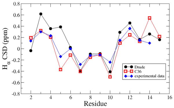
Comparison of experimental and calculated NMR Hα chemical shifts for the GB1 hairpin for the Drude (black circles) and C36 (red squares) force fields. Calculated values were from Sparta+¹¹⁹ and the experimental data corresponds to 280K while the simulations were performed at 298K.

A simulation of a dimeric coiled-coil in solution with 150 mM KCl was initiated from model 1 of the NMR structures in 1UOI,¹¹⁷ using a previously equilibrated system.⁵ Analysis involved RMS differences, φ, ψ distribution and the inter-helical angle. RMS analysis showed the overall structure of the complex to deviate more from model 1 of the NMR structure for the simulation based on the Drude-3 model (Table 7 and Figure S2b of the supporting information). This was associated with the individual helices moving relative to each other (Figure 4a), which occurs in both FFs, while the conformations of the individual helices were well preserved, indicating the ability of the model to adequately treat these essential types of secondary structure. This is supported by the φ, ψ probability distribution from the simulations (Figure S3b, supporting information). Additional analysis involved the angles between the two helices. Both the additive and polarizable models sample a range of inter-helical angles, spanning the range of values reported for the 20 models from the original NMR study. The Drude model populates a slightly wider range of angles during the 100 ns simulation, which is an indication of the additional flexibility in the model as further evidenced in the simulations of larger proteins, as presented below.

Table 7.

Average and RMS Fluctations of the RMS Differences with respect to the crystal or NMR structures of the Ca atoms for the residues in the secondary structures and for all residues. Values in Å.

Protein		Secondary				All Residues
		Average		RMS Fluc.		Average		RMS Fluc.
		Drude	C36	Drude	C36	Drude	C36	Drude	C36
A	GB1					2.70	1.28	0.49	0.47
B	IU01	1.38	1.81	0.27	0.40	1.59	2.09	0.31	0.41
C	1EJG	0.81	1.08	0.09	0.10	0.99	1.19	0.14	0.13
			1.09		0.10		1.21		0.13
D	1P7E	0.56	1.31	0.10	0.19	0.65	1.72	0.12	0.31
E	1MJC	0.51	0.57	0.08	0.09	1.56	1.65	0.19	0.26
F	1UBQ	0.72	0.95	0.11	0.14	2.17	1.67	0.69	0.31
G	3ZZP	0.98	1.33	0.11	0.15	1.48	1.64	0.15	0.19
			1.46		0.33		1.80		0.33
H	4IEJ	0.69	1.33	0.07	0.40	1.07	1.63	0.11	0.39
			1.72		0.52		2.12		0.56
I	3VQF	1.01	1.08	0.11	0.14	1.17	1.91	0.15	0.27
			1.27		0.27		1.73		0.29
J	135L	1.34	1.60	0.19	0.44	1.53	1.97	0.19	0.42
			1.59		0.31		2.19		0.34
K	1IFC	0.87	1.78	0.10	0.27	1.05	1.92	0.12	0.25
L	1BYI	1.22	1.51	0.25	0.24	1.33	2.30	0.22	0.34
			1.30		0.18		2.33		0.49

Averages over 100 ns, with the exception of 135L (93 and 100 ns) and 1BYI (100 ns). The second row for C, G, H, I, J and L is for the second Drude simulation with those systems.

Figure 4.

Helical properties in the dimeric coiled coil (1U01) simulations. A) RMS differences of the individual helix Cα atoms following alignment to themselves (eg. Helix A vs. Helix A) and following alignment based on the other helix in the dimer (eg. Helix B vs. Helix A). B) Inter-helical angle vectors defining the helical axes were calculated using the nonterminal residue Cα atoms following Chothia et al.¹³¹ NMR data for the 20 models generated in the published structural study are represented as horizontal lines

Simulations of full proteins

To further validate the Drude force field, simulations were performed on 10 additional proteins, as listed in Table 1 and shown in Figure S4, supporting information. The monomers of these proteins were subjected to ~100 ns simulations using both the polarizable and additive C36 models, with two simulations performed with the polarizable FF in select cases. The proteins were selected on the basis of coverage of secondary structure, experimental resolution, and the availability of results from previous studies. A majority of the proteins were small, being less than 100 amino acids (aa) as they would more robustly test the ability of the force field to maintain their folded structures as compared to large, globular proteins, as well as for computational expediency.

RMSD analysis was performed on all the proteins based on the Cα atoms following alignment of residues in the secondary structural elements or of all residues, with the results summarized in Table 7 and the RMSD time series for the individual systems are shown in Figure S2 of the supporting information. Table 7 also includes the RMS fluctuations of the RMSD time series. Two general trends are evident. The RMS differences are consistently smaller with the additive force field as are the RMS fluctuations. This indicates that the Drude model has additional flexibility as compared to the additive model. The only exception is the results for all residues in ubiquitin (1UBQ), where the average and fluctuations of the RMSD for all residues are larger in C36. This difference is primarily due to the 5 C-terminal residues, which have large B factors in the 1UBQ crystal structure.

Three of the proteins simulated in the present work were also studied in the recent AMOEBA protein FF paper, including crambin (1EJG), ubiquitin (1UBQ) and lysozyme (135L in the present work vs. 6LYT in the AMEOBA study).³⁶ At the end of the 30 ns simulations in the study the backbone RMSDs were approximately 1, 2 and 2 Å for the three proteins, respectively. These value compare to 1.1/1.1, 1.9 and 1.9/2.2 Å for those proteins at 30 ns of the present simulations, were two values are from the individual simulations of crambin and lysozyme. Thus, the two polarizable models yield similar RMS differences for 30 ns simulations.

While the Drude model exhibits larger flexibility as compared to the additive C36 model, the secondary structures are stable and maintained (Figure S3, supporting information). This suggests that the hydrogen bonding associated with secondary structure is being satisfactorily modeled. To verify this suggestion, the hydrogen bonding interactions involving the peptide bond N…O distance probability distributions in the helical and sheet secondary structure regions were analyzed. Shown in Figure 5 are the N…O probability distributions obtained from a subset of the simulated proteins along with survey data from crystal structures from the PDB with resolution higher than 1.5 Å.⁹⁹ With the helices, in the additive force field the distribution goes to shorter distances than observed in the survey while the agreement of the Drude model for the leading edge of the curve with the Xray data is excellent, although the maxima is the Drude model is slightly shifted back from the survey by ~0.05 Å. This difference is larger with N…O distances in the sheets, with both the additive and polarizable models having maxima longer than that in the survey, with the difference being larger in the Drude model. Thus, the Drude model gives systematically longer N…O distances than the additive model, with agreement in helices somewhat better with the Drude model, while the opposite occurs with the sheet regions. It is important to recall that the shorter distances with the additive model is consistent with the optimization of the force field, where short hydrogen bonding distances were required to yield pure solvent properties for model compounds in agreement with experiment (enthalpy and density).¹⁰ Such shortened hydrogen bond distances are not required to as great an extent with the Drude model (Table 4); however, the present results indicate that a small, systematic decrease in the distances may be required in future generations of the Drude force field.

Figure 5.

Peptide N…O distance probability distributions for the A) helical and B) sheet secondary structures from Drude (black) and C36 (red) MD simulations of the proteins 1EJG, 3VQF, 3ZZP and 4IEJ and from a survey of high-resolution crystal (xtal) structures in the Protein Databank. Probabilities were normalized to 1 and the values multiple by 100 for clarity.

Further investigation into the structural properties of the polarizable model involved analysis of the φ, ψ distributions in the studied proteins. Presented in Figure 6 are the φ, ψ inverted Boltzmann weighted distributions over protein simulations C through L reported in Table 1 with the distributions for the individual systems shown in Figure S3 of the supporting information. Figure 6 also contains a distribution obtained from the survey of the high-resolution crystal structures. Both the additive and Drude models populate regions consistent with the protein crystal structures, with the Drude model sampling a slightly wider range of φ, ψ space. In the helical region, the minimum in the Drude model is broader than with the additive model and there is additional sampling in the region of −120, 15. Both models have distributions similar to the survey results in the sheet regions, though C36 shows to more well defined minima with the Drude model exhibiting a broad, low energy region from φ = −135 to −60° for ψ ~ 150°. The Drude model also populates more of the region between the sheet and helical regions in the range of ψ = 30 to 100°. Finally, the Drude model distribution is broader in the αL region as compared to C36, consistent with the remainder of the surface, with the location of the minima in both force fields consistent with the survey data.

Figure 6.

Overall φ, ψ distributions for the A) C36 and B) Drude model and a distribution from a survey of high-resolution crystal structures. Simulated data include results from 1EJG, 1P7E, 1MJC, 1UBQ, 3ZZP, 4IEJ, 3VQF, 135L, 1IFC, and 1BYI.

The differences, as well as similarities, in the φ, ψ distributions are interesting when considered in the context of CMAP. While both the C36 and Drude surfaces have undergone some empirical adjustments, the underlying energy surfaces are based on quantum mechanics, such that the overall landscape of the surfaces should be similar. Adjustments in the C36 CMAP, which was obtained at the LMP2/cc-VQZ level included local optimization of the helical and sheet regions to reproduce subtle features observed in crystallographic survey data⁴ followed by subsequent shifting of the helical region to decrease the tendency for the C22/CMAP model to over populate that conformation, leading to C36.⁵ With the Drude model the overall sheet region was lowered and the areas between the sheet and helical regions and from φ = −90 to −180 and ψ = −60 to 105° were raised. Furthermore, we note that the conformational properties of the χ1 and χ2 side chain dihedrals were optimized with the same target function. Accordingly, the additional flexibility in the Drude model may largely be attributed to the inclusion of electronic polarization in the model. While further work is needed to understand this phenomenon, the result appears to be associated with the variability of the molecular dipoles in the Drude model, as detailed below.

NMR analysis

The above analysis largely involved the comparison of simulations of proteins in solution with experimental crystallographic data. To more carefully evaluate the behavior of the Drude model with respect to solution conditions, we calculated nuclear magnetic resonance (NMR) data, such as chemical shifts and S² order parameters, for ubiquitin (1UBQ), protein GB3 (1MJC) and cold shock protein A (1P7E). This analysis builds upon our recent comparison of the C36 force field with NMR data.^{63, 120–124} A summary of the chemical shift results for 6 different nuclei for the three proteins is presented in Table 8; results for the three proteins are shown in Table S1 of the supporting information. The overall comparison indicates that the Drude model is in poorer agreement with experiment than the highly optimized C36 model, consistent with the RMS difference analysis with respect to the crystal structures.

Table 8.

Combined RMS differences between calculated and experimental chemical shifts for ubiquitin (1UBQ), protein GB3 (1MJC) and cold shock protein A (1P7E) with the C36 additive and Drude force fields. Number of each nuclei used in the RMS difference calculations is listed.

Nucleus	# of Nuclei	RMSD (ppm)
		C36	Drude
N	192	2.50	3.21
Cα	201	0.76	1.03
Cβ	180	1.01	1.21
C′	141	0.95	0.98
H	193	0.41	0.47
Hα	201	0.23	0.30
all C	522	0.90	1.08
all H	394	0.33	0.39

Additional NMR analysis involved the calculation of peptide backbone N-H order parameters, S², for the three proteins, with the results presented on Figure 7. The results in Figure 9 for C36 are from our previous study.⁶³ For all three proteins the additive and Drude FFs are generally in similar agreement with the experimental data. Notably, the Drude model does not systematically underestimate the S² values as could have been expected given the enhanced backbone flexibility reflected in the above analyses. Moreover, in select cases, such as residues 39 to 43 of ubiquitin and 8 to 11 and 73 in protein GB3, the Drude model gives significantly larger S² values as compared to C36, with the Drude model being in better agreement with experiment. These results suggest that, while the peptide backbone is populating a wider region of φ, ψ space, the range of conformations sampled is not significantly overestimated and, in some cases, may even be more realistic than with the additive force field. Such behavior is also consistent with the proteins in the Drude force field visiting a wider range of conformations in the MD simulations, though remaining stably folded on the time scale of the presented simulations.

Figure 7.

NMR N-H backbone order parameters, S₂, from calculations using both the C36 additive and Drude force fields for A) ubiquitin (1UBQ), B) protein GB3 (1MJC) and C) Cold shock protein A (1P7E).

Figure 9.

“Unnormalized” Radial distribution function, g(r), and average dipole moments for water around (A and C) Glu64 and (B and D) Lys11 of ubiquitin. Distances based on the Glu Cε or Lys Nζ and the water oxygen and the error bars represent the RMS fluctuations.

Protein dipole moment analysis

During the development of the electrostatic aspect of the force field the partial atomic charges were put into groups of total unit charge. For example, the side chains, from the Cβ atom onward have partial atomic charges that sum to −1, 0 or 1. Similarly, the peptide bonds along with the Cα/Hα atoms have a total charge of 0. While this simplifying constraint was used to facilitate the transfer of the charges from the model compounds to the full biopolymer, it also has the advantage that it allows for the calculation of the dipole moments of the different functional groups in the MD simulations. Accordingly, analysis was performed on the dipole moments of the peptide bonds in the GB1 peptide, for the β-sheets and α-helices in ubiquitin and the Trp residues in lysozyme, which contains 6 such residues. For GB1 and lysozyme the data are presented as time series of running averages over 10 ns while the ubiquitin results are presented as probability distributions.

Analysis of the dipole moments in the backbone of GB1 shows large variability in the Drude model as compared to C36, as should be expected (Figure 8a). Variations in the additive model can only be associated with changes in the internal geometry of the peptide bond, with the occurrence of values around 4.6 D associated with the αL conformation. It is particularly noteworthy that the values are systematically higher with the Drude model—even though the dipole moments in the additive force field are systematically overestimated in order to account for the polar environment in a mean-field manner. Apparently, the results from the Drude model indicate that this overestimation of the dipoles in the additive model is insufficient to account for the relevant environments encountered by the amino acids.

Figure 8.

Dipole moment analysis (Drude, black, C36, red). A) Peptide backbone dipoles as a function of time from the GB1 hairpin simulations. B) Probability distribution of the peptide backbone dipole moments in the helices (thin lines) and β-sheets (thick lines) in ubiquitin (1UPQ). C) Tryptophan side chain dipole moments as function of time from the lysozyme (135L) Drude B simulation, with the time series for residue Trp28 and Trp123 labeled. Time series are running averages over 100 0.1 ns windows.

The peptide bond dipole moments were also analyzed with respect to secondary structure from the 1UBQ simulations. Shown in Figure 8b are probability distributions of the dipole moments in both helices and sheets for both the additive and polarizable FFs. The polarizable sheet distribution peaks in the vicinity of 5.3 D, consistent with the results for the GB1 hairpin. In the helices, the polarizable model predicts lower peptide bond dipole moments, with a maximum in the vicinity of 4.6 D. However, with the additive model, the maxima for the dipole moments are in the region of 3.7 D for both the sheets and helices, with the narrow distributions indicative of fixed charge nature of the model. We note that the dipole moment in the additive model is close to the value of 4.12 D of the additive NMA model, ³ while that in the polarizable model is 3.72 D.⁹⁶ Clearly, the present results indicate that that impact of the environment on the peptide backbone is significant, leading to significant enhancements in the local peptide bond dipole moments. Notably, these are enhancements are larger than the inherent dipole moment in the nonpolarizable additive force field, even though these moieties were “overpolarized” by designed in the parametrization of this force field. The present observation is also consistent with previous studies based on both empirical and QM methods showing the protein and aqueous environments to alter the partial atomic charges in proteins.^{26, 125, 126}

The increase in the peptide backbone dipole moments for both sheets and helices may be attributed to the hydrogen bonding interactions with surrounding peptide bonds in the secondary structures. However, the enhanced dipole moment of the sheets over the helices is somewhat unexpected. This appears to be due to the peptide dipoles pointing in opposite directions in the extended, sheet conformations, such that electrostatic interactions of peptide bond i with the adjacent i−1 and i+1 peptide bonds leads to enhancement of the peptide backbone dipole moment. This is similar to the phenomena occurring in the Drude-1 model that leads to the stabilization of the C5 conformation in (Ala)₅ discussed above (Figure 2). In helices, the i−1 and i+1 peptide bonds are approximately parallel to that of the i peptide bond so the adjacent dipole moments don’t enhance each other to as great an extent. Further studies into this observation, including the impact of changes in the electrostatic model, are warranted.

To understand the impact of the explicit inclusion of polarizability on the side chains we focus on the 6 tryptophan residues in lysozyme. Presented in Figure 8c are the dipole moments as a function of time for those residues. With the additive model, the dipole moments are in the vicinity of 2.3 D, with small variations associated with changes in intramolecular geometry, including rotations about the χ2 dihedral. In contrast, the dipole moments in the Drude model are significantly higher and fluctuate over a much wider range of values (from 2.5 to 4 D). Moreover, there are significant variations in the dipoles during the simulations, with the dipole moments of selected residues varying by more than 1 D during the simulations; analysis of individual snapshots from the simulations indicates variations from 1 to over 5 D associated with local high energy states accessible to local regions of structures during MD simulations (not shown). The tryptophan with the smallest dipole in the Drude simulation is Trp28, which is occluded from the solvent, being in contact with the side chain Trp108 (Figure S5a, supporting information). The tryptophan with the largest variation is Trp123, whose dipole moment ranges from from 2.6 to over 4 D during the simulation. This residue is solvent exposed and located adjacent to two helices (Figure S5b, supporting information), allowing it to sample different environments during the simulations, leading the variation in the dipole. As with the peptide backbone, the Drude model predicts the dipole moments of the Trp side chains to be significantly larger than in the additive force field with those dipoles being significantly different as a function of the local environment. The gas phase dipole moment of methylindole in the Drude model is 1.97,⁴⁷ compared to a value of 2.15 with the additive model,¹²⁷ indicating the significant polarization of the side chain that is occurring in the heterogenous environment of lysozyme in aqueous solution.

Water dipole moment analysis

Previous studies have shown the dipole moments of water to be perturbed in the vicinity of the protein in polarizable force field simulations.^{24, 26} Accordingly, we undertook analysis of the distribution of water molecules around the charged moieties of Glu64 and Lys11 of ubiquitin along with the change in the dipole moment of water as a function of distance (Figure 9). In both cases it may be seen that there is a perturbation of the dipole of water in the vicinity of the charged groups. With Glu64 at short distances the water dipole is decreased and there is an increase of the dipole at the first maximum of the RDF followed by a decrease at the first minimum in the RDF. With Lys11 the dipole moment of water is enhanced at the contact distance, has a minimum just beyond the peak in the g(r) followed by an increase to the bulk value of 2.45 D at longer distances. The magnitude of the changes in the dipole moments appear to be slightly smaller than previously reported,^{24, 26} which may be due scaling of the polarizable in the SWM4-NDP model by 0.7 as required to reproduce the dielectric constant of the model as well as other properties.³⁸

Practical considerations

MD simulations with a polarizable model display an enhanced sensitivity to initial conditions and are generally less robustly stable than simulations carried out with an additive force field and may display polarization catastrophes that will lead to crashes. For this reason MD simulations with a polarizable model require careful equilibration. Accordingly, the initial setup and equilibration of a simulation is best performed using an additive FF such as CHARMM36. This includes the initial solvation, minimization and dynamics in the presence of restraints on the protein, thereby allowing the solvent to relax around the protein, with the dynamics being performed in the NVT ensemble. Additional equilibration should be performed using the additive model in the NPT ensemble with the protein structure allowed to move freely or subjected to weak harmonic restraints. 100 ps of equilibration time may be sufficient, although extensive equilibration of 1 ns or more is recommended. The equilibrated system is then converted to the Drude polarizable model, including the ions and water, and subjected to an equilibration protocol similar to that initially performed using the additive model. As discussed above protein simulations with the Drude model can typically be performed with a 1 fs integration time step, though a shorter time step may be required during the initial stage of equilibration as well as for highly charged systems.

To facilitate performing MD simulations with the Drude model a new module, “Drude Prepper” has been added to the CHARMM-GUI.⁹⁰ This module allows for CHARMM additive model protein structure file (PSF) and an equilibrated coordinate files to be uploaded and then converted to Drude formatted files, including all nomenclature changes. In addition, input scripts to perform MD simulations using either CHARMM or NAMD are produced. It is anticipated that such a utility should greatly facilitate studies of proteins based on the classical Drude polarizable force field.

SUMMARY

Presented is a polarizable empirical force field based on the classical Drude oscillator for the modeling and simulation of proteins. In a first round, the parameters optimized from a large body of experimental and QM data on small model compounds representative of the all relevant protein functionalities were combined to yield a force field for the polymer. However, direct transfer of the parameters was not sufficient, requiring additional parameter optimization using larger model compounds. Most notable was the transfer of electrostatic parameters based on NMA to the polypeptide backbone. As this initial model was clearly insufficient, additional target data on the alanine dipeptide and longer polypeptides, including interactions with water, relative energies of different conformations, dipole moments and molecular polarizabilities, were used to obtain the final (Drude-3) model. In addition, final fine-tuning of the Drude-3 model required additional adjustment to the relative potential energies of different regions of φ, ψ conformational space using the CMAP term in the energy function. The resulting model was shown to yield stable explicit solvent MD simulations on the 100 nanosecond timescale for a collection of peptides and proteins. Notably, the Drude model displays more conformational flexibility than the C36 additive FF as estimated from RMS differences with respect to crystal structures and the distribution of φ, ψ conformations sampled in MD simulations. However, analysis of backbone N-H order parameters indicates that backbone fluctuations with the Drude model are not inconsistent with NMR experiments, and, in specific cases, may even represent some improvement over C36.

Both the additive C36 and polarizable Drude models targeted similar, though not identical, QM data for development of both the CMAP energy term that defines the φ, ψ potential energy surface and the dihedral parameters dictating the χ1 and χ2 side chain torsional energetics followed by additional empirical optimization of these terms. Thus, as the underlying potential energy surfaces for backbone and side chain sampling may be considered similar, the implication is that the systematically enhanced conformational flexibility of the Drude model must be associated with the electrostatic model that includes explicit induced polarization. Analysis of molecular dipoles in both the additive and Drude models shows the polarizable model gives systematically larger dipole moments for the studied moieties as compared to the nonpolarizable additive model, with those dipole moments showing significant variation during MD simulations. It therefore appears that the variations of the electronic structure do impact the dynamics of the system and the microscopic forces dictating the structural and dynamical properties of proteins. Interestingly, we note that the polarizabilities for many of the moieties in the polypeptides were scaled down relative the QM data by factors ranging from 1.0 with the aliphatics, to 0.6 with the sulfur containing groups. Indeed. The molecular polarizability of the final backbone model is systematically lower than QM estimate for the alanine dipeptide (Table 4, note that the QM values are scaled by 0.85). Thus, it seems unlikely that the current model is inherently overpolarized, though this possibility requires further study.

Overall, the current model should be considered a 1^st generation polarizable force field that can be use for MD simulations on the order of hundreds of nanoseconds. Comparison with the nonpolarizable C36 additive force field, which has had the advantage of over 20 years of testing and additional optimization since its initial completion, suggests that further improvements in the model ought to be possible. Accordingly, we anticipate that an improved 2^nd generation model can and will be produced. Nevertheless, we are confident that the current model does provide an accurate and improved picture of the structure and function of polypeptides and proteins and that it can serve as an important computational tool for the biophysical and chemical scientific communities. We also note the availability of enhancements in the model that yield more accurate treatment of cation ion-π interactions involving aromatic residues,¹²⁸ of an improved, though computationally more expensive Drude water model,³⁹ and of lipid Drude parameters⁵³ and the anticipated availability of parameters for nucleic acids (A. Savelyev and A.D. MacKerell Jr., work in progress) and carbohydrates⁵⁴ as well as tools for the optimization of small molecule parameters.¹²⁹ These enhancements and capabilities will allow for computational studies of heterogeneous systems using a fully polarizable force field.

The final residue topology information and parameters in CHARMM format may be downloaded from the MacKerell Lab Website at http://mackerell.umaryland.edu/MacKerell_Lab.html.

References

- 1.Cornell WD, Cieplak P, Bayly CI, Gould IR, Merz KM, Ferguson DM, Spellmeyer DC, Fox T, Caldwell JW, Kollman PA. A Second Generation Force Field for the Simulation of Proteins, Nucleic Acids, and Organic Molecules. J Am Chem Soc. 1995;117:5179–5197. [Google Scholar]
- 2.Wang ZX, Zhang W, Wu C, Lei H, Cieplak P, Duan Y. Strike a balance: optimization of backbone torsion parameters of AMBER polarizable force field for simulations of proteins and peptides. J Comp Chem. 2006;27:781–790. doi: 10.1002/jcc.20386. [DOI] [PMC free article] [PubMed] [Google Scholar]
- 3.MacKerell AD, Jr, Bashford D, Bellott M, Dunbrack RL, Jr, Evanseck J, Field MJ, Fischer S, Gao J, Guo H, Ha S, Joseph D, Kuchnir L, Kuczera K, Lau FTK, Mattos C, Michnick S, Ngo T, Nguyen DT, Prodhom B, Reiher IWE, Roux B, Schlenkrich M, Smith J, Stote R, Straub J, Watanabe M, Wiorkiewicz-Kuczera J, Yin D, Karplus M. All-atom empirical potential for molecular modeling and dynamics studies of proteins. J Phys Chem B. 1998;102:3586–3616. doi: 10.1021/jp973084f. [DOI] [PubMed] [Google Scholar]
- 4.MacKerell AD, Jr, Feig M, Brooks CL., III Extending the treatment of backbone energetics in protein force fields: limitations of gas-phase quantum mechanics in reproducing protein conformational distributions in molecular dynamics simulations. J Comp Chem. 2004;25:1400–1415. doi: 10.1002/jcc.20065. [DOI] [PubMed] [Google Scholar]
- 5.Best RB, Zhu X, Shim J, Lopes PEM, Mittal J, Feig M, MacKerell AD., Jr Optimization of the additive CHARMM all-atom protein force field targeting improved sampling of the backbone ϕ, ψ and side-chain χ1 and χ2 dihedral angles. J Chem Theory and Comp. 2012;8:3257–3273. doi: 10.1021/ct300400x. [DOI] [PMC free article] [PubMed] [Google Scholar]
- 6.Oostenbrink C, Soares TA, van der Vegt NFA, van Gunsteren WF. Validation of the 53A6 GROMOS force field. Eur Biophys J. 2005;34:273–284. doi: 10.1007/s00249-004-0448-6. [DOI] [PubMed] [Google Scholar]
- 7.Jorgensen WL, Tirado-Rives J. The OPLS Potential Function for Proteins. Energy Minimizations for Crystals of Cyclic Peptides and Crambin. J Am Chem Soc. 1988;110:1657–1666. doi: 10.1021/ja00214a001. [DOI] [PubMed] [Google Scholar]
- 8.Kaminski G, Friesner RA, Tirado-Rives J, Jorgensen WL. Evaluation and Reparametrization of the OPLS-AA Force Field for Proteins via Comparison with Accurate Quantum Chemical Calculations on Peptides. J Phys Chem B. 2001;105:6474–6487. [Google Scholar]
- 9.Ponder JW, Case DA. Force Fields for Protein Simulations. Adv Protein Chem. 2003;66:27–85. doi: 10.1016/s0065-3233(03)66002-x. [DOI] [PubMed] [Google Scholar]
- 10.MacKerell AD., Jr Empirical Force Fields for Biological Macromolecules: Overview and Issues. J Comp Chem. 2004;25:1584–1604. doi: 10.1002/jcc.20082. [DOI] [PubMed] [Google Scholar]
- 11.Warshel A, Levitt M. Theoretical Studies of Enzymic Reactions: Dielectric, Electrostatic and Steric Stabilization of the Carbonium Ion in the Reaction of Lysozyme. J Mol Biol. 1976;103:227–249. doi: 10.1016/0022-2836(76)90311-9. [DOI] [PubMed] [Google Scholar]
- 12.Russell ST, Warshel A. Calculations of Electrostatic Energies in Proteins: The Energetics of Ionized Groups in Bovine Pancreatic Trypsin Inhibitor. J Mol Biol. 1985;185:389–404. doi: 10.1016/0022-2836(85)90411-5. [DOI] [PubMed] [Google Scholar]
- 13.van Belle D, Couplet I, Prevost M, Wodak SJ. Calculations of Electrostatic Properties in Proteins - Analysis of Contributions from Induced Protein Dipoles. J Mol Biol. 1987;198:721–735. doi: 10.1016/0022-2836(87)90213-0. [DOI] [PubMed] [Google Scholar]
- 14.Halgren TA, Damm W. Polarizable force fields. Curr Opin Struct Biol. 2001;11:236–242. doi: 10.1016/s0959-440x(00)00196-2. [DOI] [PubMed] [Google Scholar]
- 15.Rick SW, Stuart SJ. Potentials and Algorithms for Incorporating Polarizability in Computer Simulations. Rev Comp Chem. 2002;18:89–146. [Google Scholar]
- 16.Warshel A, Kato M, Pisliakov AV. Polarizable Force Fields: History, Test Cases, and Prospects. Journal of Chemical Theory and Computation. 2007;3:2034–2045. doi: 10.1021/ct700127w. [DOI] [PubMed] [Google Scholar]
- 17.Lopes PEM, Roux B, MacKerell AD., Jr Molecular modeling and dynamics studies with explicit inclusion of electronic polarizability: theory and applications. Theor Chem Acc. 2009;124:11–28. doi: 10.1007/s00214-009-0617-x. [DOI] [PMC free article] [PubMed] [Google Scholar]
- 18.Cieplak P, Dupradeau F-Y, Duan Y, Wang J. Polarization effects in molecular mechanical force fields. J Phys: Condens Matter. 2009;21:333102. doi: 10.1088/0953-8984/21/33/333102. [DOI] [PMC free article] [PubMed] [Google Scholar]
- 19.Banks JL, Kaminski GA, Zhou R, Mainz DT, Berne BJ, Friesner RA. Parametrizing a Polarizable Force Field from Ab Initio Data. I. The Fluctuating Point Charge Model. J Chem Phys. 1999;110:741–754. [Google Scholar]
- 20.Stern HA, Kaminski GA, Banks JL, Zhou R, Berne BJ, Friesner RA. Fluctuating Charge, Polarizable Dipole, and Combined Models: Parameterization from ab Initio Quantum Chemistry. J Phys Chem B. 1999;103:4730–4737. [Google Scholar]
- 21.Stern HA, Rittner F, Berne BJ, Friesner RA. Combined fluctuating charge and polarizable dipole models: Application to a five-site water potential function. J Chem Phys. 2001;115:2237–2251. [Google Scholar]
- 22.Kaminski GA, Stern HA, Berne BJ, Friesner RA, Cao YX, Murphy RB, Zhou R, Halgren TA. Development of a Polarizable Force Field for Proteins via Ab Initio Quantum Chemistry: First Generation Model and Gas Phase Tests. J Comp Chem. 2002;23:1515–1531. doi: 10.1002/jcc.10125. [DOI] [PMC free article] [PubMed] [Google Scholar]
- 23.Harder E, Kim B, Friesner RA, Berne BJ. Efficient Simulation Method for Polarizable Protein Force Fields: Application to the Simulation of BPTI in Liquid Water. J Chem Theory Comp. 2005;1:169–180. doi: 10.1021/ct049914s. [DOI] [PubMed] [Google Scholar]
- 24.Kim B, Young T, Harder E, Friesner RA, Berne BJ. Structure and Dynamics of the Solvation of Bovine Pancreatic Trypsin Inhibitor in Explicit Water: A Comparitive Study of the Effects of Solvent and Protein Polarizability. J Phys Chem B. 2005;109:16529–16538. doi: 10.1021/jp051569v. [DOI] [PMC free article] [PubMed] [Google Scholar]
- 25.Patel S, Brooks CL., III CHARMM fluctuating charge force field for proteins: I parameterization and application to bulk organic liquid simulations. J Comp Chem. 2004;25:1–15. doi: 10.1002/jcc.10355. [DOI] [PubMed] [Google Scholar]
- 26.Patel S, MacKerell AD, Jr, Brooks CL., III CHARMM fluctuating charge force field for proteins: II Protein/solvent properties from molecular dynamics simulations using a nonadditive electrostatic model. J Comp Chem. 2004;25:1504–1514. doi: 10.1002/jcc.20077. [DOI] [PubMed] [Google Scholar]
- 27.Ren P, Ponder JW. Consistent Treatment of Inter- and Intramolecular Polarization in Molecular Mechanics Calculations. J Comp Chem. 2002;23:1497–1506. doi: 10.1002/jcc.10127. [DOI] [PubMed] [Google Scholar]
- 28.Ponder JW, Wu C, Ren P, Pande VS, Chodera JD, Schnieders MJ, Haque I, Mobley DL, Lambrecht DS, DiStasio RA, Jr, Head-Gordon M, Clark GN, Johnson ME, Head-Gordon T. Current status of the AMOEBA polarizable force field. J Phys Chem B. 2010;114:2549–2564. doi: 10.1021/jp910674d. [DOI] [PMC free article] [PubMed] [Google Scholar]
- 29.Jiao D, Golubkov PA, Darden TA, Ren P. Calculation of protein-ligand binding free energy by using a polarizable potential. Proc Natl Acad Sci USA. 2008;105:6290–6295. doi: 10.1073/pnas.0711686105. [DOI] [PMC free article] [PubMed] [Google Scholar]
- 30.Jiao D, Zhang J, Duke RE, Li G, Schnieders MJ, Ren P. Trypsin-ligand binding free energies from explicit and implicit solvent simulations with polarizable potential. J Comp Chem. 2009;30:1701–1711. doi: 10.1002/jcc.21268. [DOI] [PMC free article] [PubMed] [Google Scholar]
- 31.Shi Y, Zhu CZ, Martin SF, Ren P. Probing the Effect of Conformational Constraint on Phosphorylated Ligand Binding to an SH2 Domain Using Polarizable Force Field Simulations. J Phys Chem B. 2012;116:1716–1727. doi: 10.1021/jp210265d. [DOI] [PMC free article] [PubMed] [Google Scholar]
- 32.Zhang J, Yang W, Piquemal JP, Ren P. Modeling Structural Coordination and Ligand Binding in Zinc Proteins with a Polarizable Potential. J Chem Theory and Comp. 2012;8:1314–1324. doi: 10.1021/ct200812y. [DOI] [PMC free article] [PubMed] [Google Scholar]
- 33.Schultheis V, Reichold R, Schropp B, Tavan P. A Polarizable Force Field for Computing the Infrared Spectra of the Polypeptide Backbone. J Phys Chem B. 2008;112:12217–12230. doi: 10.1021/jp8013767. [DOI] [PubMed] [Google Scholar]
- 34.Click TH, Kaminski GA. Reproducing basic pKa values for turkey ovomucoid third domain using a polarizable force field. J Phys Chem B. 2009;113:7844–7850. doi: 10.1021/jp809412e. [DOI] [PMC free article] [PubMed] [Google Scholar]
- 35.Zhong Y, Patel S. Binding structures of tri-N-acetyl-beta-glucosamine in hen egg white lysozyme using molecular dynamics with a polarizable force field. J Comp Chem. 2013;34:163–174. doi: 10.1002/jcc.23109. [DOI] [PMC free article] [PubMed] [Google Scholar]
- 36.Shi Y, Xia Z, Zhang J, Best R, Wu C, Ponder JW, Ren P. Polarizable Atomic Multipole-Based AMEOPA Force Field for Proteins. J Chem Theory and Comp. 2013;9:4046–4064. doi: 10.1021/ct4003702. [DOI] [PMC free article] [PubMed] [Google Scholar]
- 37.Lamoureux G, MacKerell AD, Jr, Roux B. A simple polarizable model of water based on classical Drude oscillators. J Chem Phys. 2003;119:5185–5197. [Google Scholar]
- 38.Lamoureux G, Harder E, Vorobyov IV, Roux B, MacKerell AD., Jr A polarizable model of water for molecular dynamics simulations of biomolecules. Chem Phys Lett. 2006;418:245–249. [Google Scholar]
- 39.Yu W, Lopes PE, Roux B, MacKerell AD., Jr Six-site polarizable model of water based on the classical Drude oscillator. J Chem Phys. 2013;138:034508. doi: 10.1063/1.4774577. [DOI] [PMC free article] [PubMed] [Google Scholar]
- 40.Vorobyov I, Anisimov VM, Greene S, Venable RM, Moser A, Pastor RW, MacKerell AD., Jr Additive and Classical Drude Polarizable Force Fields for Linear and Cyclic Ethers. J Chem Theory Comp. 2007;3:1120–1133. doi: 10.1021/ct600350s. [DOI] [PubMed] [Google Scholar]
- 41.Harder E, Anisimov VM, Whitfield T, MacKerell AD, Jr, Roux B. Understanding the Dielectric Properties of Liquid Amides from a Polarizable Force Field. J Phys Chem B. 2008;112:3509–3521. doi: 10.1021/jp709729d. [DOI] [PMC free article] [PubMed] [Google Scholar]
- 42.Lopes PEM, Lamoureux G, Roux B, MacKerell AD., Jr Polarizable Empirical Force Field for Aromatic Compounds Based on the Classical Drude Oscillator. J Phys Chem B. 2007;111:2873–2885. doi: 10.1021/jp0663614. [DOI] [PMC free article] [PubMed] [Google Scholar]
- 43.Anisimov VM, Vorobyov IV, Roux B, MacKerell AD., Jr Polarizable empirical force field for the primary and secondary alcohol series based on the classical Drude model. J Chem Theory Comp. 2007;3:1927–1946. doi: 10.1021/ct700100a. [DOI] [PMC free article] [PubMed] [Google Scholar]
- 44.Harder E, Anisimov VM, Vorobyov IV, Lopes PEM, Noskov S, MacKerell AD, Jr, Roux B. Atomic Level Anisotropy in the Electrostatic Modeling of Lone Pairs for a Polarizable Force Field based on the Classical Drude Oscillator. J Chem Theory Comp. 2006;2:1587–1597. doi: 10.1021/ct600180x. [DOI] [PubMed] [Google Scholar]
- 45.Zhu X, MacKerell AD., Jr Polarizable empirical force field for sulfur-containing compounds based on the classical Drude oscillator model. J Comp Chem. 2010;31:2330–2341. doi: 10.1002/jcc.21527. [DOI] [PMC free article] [PubMed] [Google Scholar]
- 46.Baker CM, MacKerell AD., Jr Polarizability rescaling and atom-based Thole scaling in the CHARMM Drude polarizable force field for ethers. J Mol Model. 2010;16:567–576. doi: 10.1007/s00894-009-0572-4. [DOI] [PMC free article] [PubMed] [Google Scholar]
- 47.Lopes PEM, Lamoureux G, MacKerell AD., Jr Polarizable Empirical Force Field for Nitrogen-containing Heteroaromatic Compounds Based on the Classical Drude Oscillator. J Comp Chem. 2009;30:1821–1838. doi: 10.1002/jcc.21183. [DOI] [PMC free article] [PubMed] [Google Scholar]
- 48.Baker CM, Anisimov VM, MacKerell AD., Jr Development of CHARMM Polarizable Force Field for Nucleic Acid Bases Based on the Classical Drude Oscillator Model. J Phys Chem B. 2011;115:580–596. doi: 10.1021/jp1092338. [DOI] [PMC free article] [PubMed] [Google Scholar]
- 49.Yu H, Whitfield TW, Harder E, Lamoureux G, Vorobyov I, Anisimov VM, MacKerell AD, Jr, Roux B. Simulating Monovalent and Divalent Ions in Aqueous Solution Using a Drude Polarizable Force Field. J Chem Theory Comp. 2010;6:774–786. doi: 10.1021/ct900576a. [DOI] [PMC free article] [PubMed] [Google Scholar]
- 50.Luo Y, Jiang W, Yu H, MacKerell AD, Jr, Roux B. Simulation study of ion pairing in concentrated aqueous salt solutions with a polarizable force field. Faraday Discussions. 2013;160:135– 149. doi: 10.1039/c2fd20068f. [DOI] [PMC free article] [PubMed] [Google Scholar]
- 51.Anisimov VM, Lamoureux G, Vorobyov IV, Huang N, Roux B, MacKerell AD., Jr Determination of Electrostatic Parameters for a Polarizable Force Field Based on the Classical Drude Oscillator. J Chem Theory Comp. 2005;1:153–168. doi: 10.1021/ct049930p. [DOI] [PubMed] [Google Scholar]
- 52.Harder E, MacKerell AD, Jr, Roux B. Electronic Polarization Effects and the Membrane Dipole Potential. J Am Chem Soc. 2009;131:2760–2761. doi: 10.1021/ja806825g. [DOI] [PMC free article] [PubMed] [Google Scholar]
- 53.Chowdhary J, Harder E, Lopes PE, Huang L, MacKerell AD, Jr, Roux B. A Polarizable Force Field of Dipalmitoylphosphatidylcholine Based on the Classical Drude Model for Molecular Dynamics Simulations of Lipids. J Phys Chem B. 2013;117:9142–9160. doi: 10.1021/jp402860e. [DOI] [PMC free article] [PubMed] [Google Scholar]
- 54.He X, Lopes PEM, MacKerell AD., Jr Polarizable Empirical Force Field for Acyclic Poly-Alcohols Based on the Classical Drude Oscillator. Biopolymers. 2013;99:724–738. doi: 10.1002/bip.22286. [DOI] [PMC free article] [PubMed] [Google Scholar]
- 55.Best RB, Mittal J. Balance between alpha and beta structures in ab initio protein folding. J Phys Chem B. 2010;114:8790–8798. doi: 10.1021/jp102575b. [DOI] [PubMed] [Google Scholar]
- 56.Best RB, Mittal J. Protein simulations with an optimized water model: cooperative helix formation and temperature-induced unfolded state collapse. J Phys Chem B. 2010;114:14916–14923. doi: 10.1021/jp108618d. [DOI] [PubMed] [Google Scholar]
- 57.Best RB, Buchete NV, Hummer G. Are current molecular dynamics force fields too helical? Biophys J. 2008;95:L07–09. doi: 10.1529/biophysj.108.132696. [DOI] [PMC free article] [PubMed] [Google Scholar]
- 58.Shaw DE, Maragakis P, Lindorff-Larsen K, Piana S, Dror RO, Eastwood MP, Bank JA, Jumper JM, Salmon JK, Shan Y, Wriggers W. Atomic-level characterization of the structural dynamics of proteins. Science. 2010;330:341–346. doi: 10.1126/science.1187409. [DOI] [PubMed] [Google Scholar]
- 59.Piana S, Lindorff-Larsen K, Shaw DE. How robust are protein folding simulations with respect to force field parameterization? Biophys J. 2011;100:L47–49. doi: 10.1016/j.bpj.2011.03.051. [DOI] [PMC free article] [PubMed] [Google Scholar]
- 60.Lindorff-Larsen K, Maragakis P, Piana S, Eastwood MP, Dror RO, Shaw DE. Systematic validation of protein force fields against experimental data. PLoS ONE. 2012;7:e32131. doi: 10.1371/journal.pone.0032131. [DOI] [PMC free article] [PubMed] [Google Scholar]
- 61.Piana S, Lindorff-Larsen K, Dirks RM, Salmon JK, Dror RO, Shaw DE. Evaluating the effects of cutoffs and treatment of long-range electrostatics in protein folding simulations. PLoS ONE. 2012;7:e39918. doi: 10.1371/journal.pone.0039918. [DOI] [PMC free article] [PubMed] [Google Scholar]
- 62.Best RB, Mittal J, Feig M, MacKerell AD., Jr Inclusion of many-body effects in the additive CHARMM protein CMAP potential results in enhanced cooperativity of alpha-helix and beta-hairpin formation. Biophysical Journal. 2012;103:1045–1051. doi: 10.1016/j.bpj.2012.07.042. [DOI] [PMC free article] [PubMed] [Google Scholar]
- 63.Huang J, MacKerell AD., Jr CHARMM36 all-atom additive protein force field: Validation based on comparison to NMR data. J Comp Chem. 2013;34:2135–2145. doi: 10.1002/jcc.23354. [DOI] [PMC free article] [PubMed] [Google Scholar]
- 64.van Marren PJ, van der Spoel D. Molecular Dynamics Simulations of Water with Novel Shell-Model Potentials. J Phys Chem B. 2001;105:2618–2626. [Google Scholar]
- 65.Kunz AP, van Gunsteren WF. Development of a nonlinear classical polarization model for liquid water and aqueous solutions: COS/D. J Phys Chem A. 2009;113:11570–11579. doi: 10.1021/jp903164s. [DOI] [PubMed] [Google Scholar]
- 66.Drude P, Millikan RA, Mann RC. The Theory of Optics. Longmans, Green, and Co; New York: 1902. p. 588. [Google Scholar]
- 67.Waldman M, Gordon RG. Generalized electron gas-Drude model theory of intermolecular forces. J Chem Phys. 1979;71:1340–1352. [Google Scholar]
- 68.Applequist J, Carl JR, Fung K-K. Atom dipole interaction model for molecular polarizability. Application to polyatomic molecules and determination of atom polarizabilities. J Am Chem Soc. 1972;94:2952–2960. [Google Scholar]
- 69.Thole BT. Molecular polarizabilities calculated with a modified dipole interaction. Chem Phys. 1981;59:341–350. [Google Scholar]
- 70.Lopes PEM, Harder E, Roux B, MacKerell AD., Jr . Formalisms for the explicit inclusion of electronic polarizability in molecular modeling and dynamics studies. In: York D, Lee T-S, editors. Multi-scale Quantum Models for Biocatalysis: Modern Techniques and Applications. 2009. [Google Scholar]
- 71.Sprik M, Klein ML. A Polarizable Model for Water Using Distributed Charge Sites. J Chem Phys. 1988;89:7556–7560. [Google Scholar]
- 72.Martyna GJ, Tuckerman ME, Tobias DJ, Klein ML. Explicit reversible integrators for extended systems dynamics. Mol Phys. 1996;87:1117–1157. [Google Scholar]
- 73.Tuckerman ME, Martyna GJ. Understanding Modern Molecular Dynamics: Techniques and Applications. J Phys Chem B. 2000;104:159–178. [Google Scholar]
- 74.Lamoureux G, Roux B. Modelling Induced Polarizability with Drude Oscillators: Theory and Molecular Dynamics Simulation Algorithm. J Chem Phys. 2003;119:5185–5197. [Google Scholar]
- 75.Jiang W, Hardy DJ, Phillips JC, Mackerell AD, Jr, Schulten K, Roux B. High-performance scalable molecular dynamics simulations of a polarizable force field based on classical Drude oscillators in NAMD. J Phys Chem Lett. 2011;2:87–92. doi: 10.1021/jz101461d. [DOI] [PMC free article] [PubMed] [Google Scholar]
- 76.Frisch MJ, Trucks GW, Schlegel HB, Scuseria GE, Robb MA, Cheeseman JR, Scalmani G, Barone V, Mennucci B, Petersson GA, Nakatsuji H, Caricato M, Li X, Hratchian HP, Izmaylov AF, Bloino J, Zheng G, Sonnenberg JL, Hada M, Ehara M, Toyota K, Fukuda R, Hasegawa J, Ishida M, Nakajima T, Honda Y, Kitao O, Nakai H, Vreven T, Montgomery J, JA, Peralta JE, Ogliaro F, Bearpark M, Heyd JJ, Brothers E, Kudin KN, Staroverov VN, Kobayashi R, Normand J, Raghavachari K, Rendell A, Burant JC, Iyengar SS, Tomasi J, Cossi M, Rega N, Millam NJ, Klene M, Knox JE, Cross JB, Bakken V, Adamo C, Jaramillo J, Gomperts R, Stratmann RE, Yazyev O, Austin AJ, Cammi R, Pomelli C, Ochterski JW, Martin RL, Morokuma K, Zakrzewski VG, Voth GA, Salvador P, Dannenberg JJ, Dapprich S, Daniels AD, Farkas Ö, Foresman JB, Ortiz JV, Cioslowski J, Fox DJ. Gaussian 09. Gaussian, Inc; Wallingford CT: 2009. [Google Scholar]
- 77.Shao Y, Fusti-Molnar L, Jung Y, Kussmann J, Ochsenfeld C, Brown ST, Gilbert ATB, Slipchenko LV, Levchenko SV, O’Neill DP, Jr, RAD, Lochan RC, Wang T, Beran GJO, Besley NA, Herbert JM, Lin CY, Voorhis TV, Chien SH, Sodt A, Steele RP, Rassolov VA, Maslen PE, Korambath PP, Adamson RD, Austin B, Baker J, Byrd EFC, Dachsel H, Doerksen RJ, Dreuw A, Dunietz BD, Dutoi AD, Furlani TR, Gwaltney SR, Heyden A, Hirata S, Hsu C-P, Kedziora G, Khalliulin RZ, Klunzinger P, Lee AM, Lee MS, Liang W, Lotan I, Nair N, Peters B, Proynov EI, Pieniazek PA, Rhee YM, Ritchie J, Rosta E, Sherrill CD, Simmonett AC, Subotnik JE, III, HLW, Zhang W, Bell AT, Chakraborty AK, Chipman DM, Keil FJ, Warshel A, Hehre WJ, III, HFS, Kong J, Krylov AI, Gill PMW, Head-Gordon M, Gan Z, Zhao Y, Schultz NE, Truhlar D, Epifanovsky E, Oana M. Q-Chem Q-Chem 31. Q-Chem, Inc; Pittsburgh, PA: 2007. [Google Scholar]
- 78.Kong J, White CA, Krylov AI, Sherrill CD, Adamson RD, Furlani TR, Lee MS, Lee AM, Gwaltney SR, Adams TR, Ochsenfeld C, Gilbert ATB, Kedziora GS, Rassolov VA, Maurice DR, Nair N, Shao Y, Besley NA, Maslen PE, Dombroski JP, Daschel H, Zhang W, Korambath PP, Baker J, Byrd EFC, Voorhis TV, Oumi M, Hirata S, Hsu C-P, Ishikawa N, Florian J, Warshel A, Johnson BG, Gill PMW, Head-Gordon M, Pople JA. Q-Chem 2.0: A high-performance ab initio electronic structure program. J Comput Chem. 2000;21:1532–1548. [Google Scholar]
- 79.Woon DE, Dunning TH., Jr Gaussian basis sets for use in correlated molecular calculations. III. The atoms aluminum through argon. J Chem Phys. 1993;98:1358–1371. [Google Scholar]
- 80.Møller C, Plesset MS. Note on an Approximation Treatment for Many-Electron Systems. Phys Rev. 1934;46:618–622. [Google Scholar]
- 81.Halkier A, Helgakerb T, Jørgensena P, Klopperb W, Kocha H, Olsenc J, Wilson AK. Basis-set convergence in correlated calculations on Ne, N2, and H2O. Chem Phys Let. 1998;286:243–252. [Google Scholar]
- 82.Brooks BR, Brooks CL, 3rd, MacKerell AD, Jr, Nilsson L, Petrella RJ, Roux B, Won Y, Archontis G, Bartels C, Boresch S, Caflisch A, Caves L, Cui Q, Dinner AR, Feig M, Fischer S, Gao J, Hodoscek M, Im W, Kuczera K, Lazaridis T, Ma J, Ovchinnikov V, Paci E, Pastor RW, Post CB, Pu JZ, Schaefer M, Tidor B, Venable RM, Woodcock HL, Wu X, Yang W, York DM, Karplus M. CHARMM: the biomolecular simulation program. J Comp Chem. 2009;30:1545–1614. doi: 10.1002/jcc.21287. [DOI] [PMC free article] [PubMed] [Google Scholar]
- 83.MacKerell AD, Jr, Brooks B, Brooks CL, III, Nilsson L, Roux B, Won Y, Karplus M. CHARMM: The Energy Function and Its Paramerization with an Overview of the Program. In: Schleyer PvR, Allinger NL, Clark T, Gasteiger J, Kollman PA, Schaefer HF, III, Schreiner PR., editors. Encyclopedia of Computational Chemistry. Vol. 1. John Wiley & Sons; Chichester: 1998. pp. 271–277. [Google Scholar]
- 84.Brooks BR, Bruccoleri RE, Olafson BD, States DJ, Swaminathan S, Karplus M. CHARMM: A Program for Macromolecular Energy, Minimization, and Dynamics Calculations. J Comp Chem. 1983;4:187–217. [Google Scholar]
- 85.Allen MP, Tildesley DJ. Computer Simulation of Liquids. Oxford University Press; New York: 1989. [Google Scholar]
- 86.Ryckaert JP, Ciccotti G, Berendsen HJC. Numerical Integration of the Cartesian Equations of Motion of a System with Constraints: Molecular Dynamics of n-alkanes. J Comp Phys. 1977;23:327–341. [Google Scholar]
- 87.Miyamoto S, Kollman P. SETTLE: An Analytical Version of the SHAKE and RATTLE Algorithm for Rigid Water Models. J Comput Chem. 1992;13:952–962. [Google Scholar]
- 88.Berman HM, Battistuz T, Bhat TN, Bluhm WF, Bourne PE, Burkhardt K, Feng Z, Gilliland GL, Iype L, Jain S, Fagan P, Marvin J, Padilla D, Ravichandran V, Schneider B, Thanki N, Weissig H, Westbrook JD, Zardecki C. The protein data bank. Acta Crystallogr D Biol Crystallogr. 2002;58:899–907. doi: 10.1107/s0907444902003451. [DOI] [PubMed] [Google Scholar]
- 89.Jorgensen WL, Chandrasekhar J, Madura JD, Impey RW, Klein ML. Comparison of Simple Potential Functions for Simulating Liquid Water. J Chem Phys. 1983;79:926–935. [Google Scholar]
- 90.Jo S, Kim T, Iyer VG, Im W. CHARMM-GUI: a web-based graphical user interface for CHARMM. J Comp Chem. 2008;29:1859–1865. doi: 10.1002/jcc.20945. [DOI] [PubMed] [Google Scholar]
- 91.Fukunishi H, Watanabe O, Takada S. On the Hamiltonian replica exchange method for efficient sampling of biomolecular systems: Application to protein structure prediction. J Chem Phys. 2002;116:9058. [Google Scholar]
- 92.Graf J, Nguyen PH, Stock G, Schwalbe H. Structure and dynamics of the homologous series of alanine peptides: A joint molecular dynamics/NMR study. J Am Chem Soc. 2007;129:1179–1189. doi: 10.1021/ja0660406. [DOI] [PubMed] [Google Scholar]
- 93.Metropolis N, Rosenbluth AW, Rosenbluth MN, Teller AH, Teller E. Equation of State Calculations by Fast Computing Machines. J Chem Phys. 1953;21:1087–1092. [Google Scholar]
- 94.Hansmann UHE. Parallel tempering algorithm for conformational studies of biological molecules. Chem Phys Lett. 1997;281:140–150. [Google Scholar]
- 95.Sugita Y, Kitao A, Okamoto Y. Multidimensional replica-exchange method for free-energy calculations. J Chem Phys. 2000;113:6042–6051. [Google Scholar]
- 96.Lin B, Lopes PEM, Roux B, MacKerell AD., Jr Kirkwood-Buff Analysis of Aqueous N-Methylacetamide and Acetamide Solutions Modeled by the CHARMM Additive and Drude Polarizable Force Fields. J Chem Phys. 2013;139:084509. doi: 10.1063/1.4818731. [DOI] [PMC free article] [PubMed] [Google Scholar]
- 97.Miller KJ. Additivity Methods in Molecular Polarizability. J Am Chem Soc. 1990;112:8533–8542. [Google Scholar]
- 98.Kirkpatrick S, Gelatt CDJ, Vecchi MP. Optimization by Simulated Annealing. Science. 1983;220:671–680. doi: 10.1126/science.220.4598.671. [DOI] [PubMed] [Google Scholar]
- 99.Zhu X, Lopes PE, Shim J, MacKerell AD., Jr Intrinsic energy landscapes of amino acid side-chains. J Chem Inf Model. 2012;52:1559–1572. doi: 10.1021/ci300079j. [DOI] [PMC free article] [PubMed] [Google Scholar]
- 100.Guvench O, MacKerell AD., Jr Automated conformational energy fitting for force-field development. J Mol Mod. 2008;14:667–679. doi: 10.1007/s00894-008-0305-0. [DOI] [PMC free article] [PubMed] [Google Scholar]
- 101.Wang L, Friesner RA, Berne BJ. Replica exchange with solute scaling: a more efficient version of replica exchange with solute tempering (REST2) J Phys Chem B. 2011;115:9431–9438. doi: 10.1021/jp204407d. [DOI] [PMC free article] [PubMed] [Google Scholar]
- 102.Liu P, Kim B, Friesner RA, Berne BJ. Replica exchange with solute tempering: A method for sampling biological systems in explicit water. Proc Nat Acad Sci USA. 2005;102:13749–13754. doi: 10.1073/pnas.0506346102. [DOI] [PMC free article] [PubMed] [Google Scholar]
- 103.Bernard D, Coop A, MacKerell AD., Jr 2D Conformationally Sampled Pharmacophore: A Ligand-Based Pharmacophore To Differentiate delta Opioid Agonists from Antagonists. J Am Chem Soc. 2003;125:3101–3107. doi: 10.1021/ja027644m. [DOI] [PubMed] [Google Scholar]
- 104.Foloppe N, MacKerell AD., Jr All-atom empirical force field for nucleic acids: 1) Parameter optimization based on small molecule and condensed phase macromolecular target data. J Comp Chem. 2000;21:86–104. [Google Scholar]
- 105.Oostenbrink C, Villa A, Mark AE, van Gunsteren WF. A Biomolecular Force Field Based on the Free Enthalpy of Hydration and Solvation: The GROMOS Force-Field Parameter Sets 53A5 and 53A6. J Comp Chem. 2004;25:1656–1676. doi: 10.1002/jcc.20090. [DOI] [PubMed] [Google Scholar]
- 106.MacKerell AD, Jr, Feig M, Brooks CL., III Accurate treatment of protein backbone conformational energetics in empirical force fields. J Am Chem Soc. 2004;126:698–699. doi: 10.1021/ja036959e. [DOI] [PubMed] [Google Scholar]
- 107.Shoemaker KR, Kim PS, Brems DN, Marqusee S, York EJ, Chaiken IM, Stewart JM, Baldwin RL. Nature of the Charged-Group Effect on the Stability of the C-Peptide Helix. Proc Nat Acad Sci USA. 1985;82:2349–2353. doi: 10.1073/pnas.82.8.2349. [DOI] [PMC free article] [PubMed] [Google Scholar]
- 108.Shoemaker KR, Kim PS, York EJ, Stewart JM, Baldwin RL. Tests of the Helix Dipole Model for Stabilization of α-Helices. Nature. 1987;326:563–567. doi: 10.1038/326563a0. [DOI] [PubMed] [Google Scholar]
- 109.Padmanabhan S, Marqusee S, Ridgeway T, Laue TM, Baldwin RL. Relative Helix-Forming Tendencies of Nonpolar Amino Acids. Nature. 1990;344:268–270. doi: 10.1038/344268a0. [DOI] [PubMed] [Google Scholar]
- 110.Dunbrack RL, Karplus M. Backbone-Dependent Rotamer Library for Proteins. Application to Side-Chain Prediction. J Mol Biol. 1993;230:543–574. doi: 10.1006/jmbi.1993.1170. [DOI] [PubMed] [Google Scholar]
- 111.Dunbrack RL, Jr, Cohen FE. Bayesian statistical analysis of protein sidechain rotamer preferences. Prot Sci. 1997;6:1661–1681. doi: 10.1002/pro.5560060807. [DOI] [PMC free article] [PubMed] [Google Scholar]
- 112.Dunbrack RL., Jr . Culledpdb: Non-redundant set of protein sidechains from the PDB. Philadelphia: 2002. http://www.fccc.edu/research/labs/dunbrack/culledpdb.html. [Google Scholar]
- 113.Lindorff-Larsen K, Piana S, Palmo K, Maragakis P, Klepeis JL, Dror RO, Shaw DE. Improved side-chain torsion potentials for the Amber ff99SB protein force field. Proteins. 2010;78:1950–1958. doi: 10.1002/prot.22711. [DOI] [PMC free article] [PubMed] [Google Scholar]
- 114.Shim J, Zhu X, Best RB, MacKerell AD., Jr (Ala)(4)-X-(Ala)4 as a model system for the optimization of the chi1 and chi2 amino acid side-chain dihedral empirical force field parameters. J Comp Chem. 2013;34:593–603. doi: 10.1002/jcc.23178. [DOI] [PMC free article] [PubMed] [Google Scholar]
- 115.Blanco FJ, Rivas G, Serrano L. A short linear peptide that folds into a native stable bold beta-hairpin in aqueous solution. Nat Struct Biol. 1994;1:584–590. doi: 10.1038/nsb0994-584. [DOI] [PubMed] [Google Scholar]
- 116.Muñoz V, Thompson PA, Hofrichter J, Eaton WA. Folding Dynamics and Mechanism of β-Hairpin Formation. Nature. 1997;390:196–199. doi: 10.1038/36626. [DOI] [PubMed] [Google Scholar]
- 117.Schuler B, Eaton WA. Protein folding studied by single molecule. Curr Opin Struct Biol. 2008;18:16–26. doi: 10.1016/j.sbi.2007.12.003. [DOI] [PMC free article] [PubMed] [Google Scholar]
- 118.Fesinmeyer RM, Hudson FM, Andersen NH. Enhanced hairpin stability through loop design: the case of the protein G B1 domain hairpin. J Am Chem Soc. 2004;126:7238–7243. doi: 10.1021/ja0379520. [DOI] [PubMed] [Google Scholar]
- 119.Shen Y, Bax A. SPARTA+: a modest improvement in empirical NMR chemical shift prediction by means of an artificial neural network. J Biomol NMR. 2010;48:13–22. doi: 10.1007/s10858-010-9433-9. [DOI] [PMC free article] [PubMed] [Google Scholar]
- 120.Tjandra N, Feller SE, Pastor RW, Bax A. Rotational diffusion anisotropy of human ubiquitin from 15N NMR relaxation. J Am Chem Soc. 1995;117:12562–12566. [Google Scholar]
- 121.Hodsdon ME, Cistola DP. Backbone Mobility of Intestinal Fatty Acid-Binding Protein as Monitored by 15N NMR Relaxation and 1H Exchange. Biochem. 1997;36:2278–2290. doi: 10.1021/bi962018l. [DOI] [PubMed] [Google Scholar]
- 122.Cornilescu G, Marquardt JL, Ottiger M, Bax A. Validation of Protein Structure from Anisotropic Carbonyl Chemical Shifts in a Dilute Liquid Crystalline Phase. J Am Chem Soc. 1998;120:6836–6837. [Google Scholar]
- 123.Feng W, Tejero R, Zimmerman DE, Inouye M, Montelione GT. Solution NMR Structure and Backbone Dynamics of the Major Cold-Shock Protein (CspA) from Escherichia coli: Evidence for Conformational Dynamics in the Single-Stranded RNA-Binding Site. Biochem. 1998;37:10881–10896. doi: 10.1021/bi980269j. [DOI] [PubMed] [Google Scholar]
- 124.Vögeli B, Kazemi S, Güntert P, Riek R. Spatial elucidation of motion in proteins by ensemble-based structure calculation using exact NOEs. Nat Struct Mol Biol. 2012;19:1053–1057. doi: 10.1038/nsmb.2355. [DOI] [PubMed] [Google Scholar]
- 125.van der Vaart A, Merz JKM. The Role of Polarization and Charge Transfer in the Solvation of Biomolecules. J Amer Chem Soc. 1999;121:9182–9190. [Google Scholar]
- 126.van der Vaart A, Bursulaya BD, Brooks CL, Merz KM. Are Many-Body Effects Important in Protein Folding? J Phys Chem B. 2000;104:9554–9563. [Google Scholar]
- 127.Macias AT, MacKerell AD., Jr CH/pi Interactions involving Aromatic Amino Acids: Refinement of the CHARMM Tryptophan Force Field. J Comp Chem. 2005;26:1452–1463. doi: 10.1002/jcc.20281. [DOI] [PubMed] [Google Scholar]
- 128.Wang S, Orabi EA, Baday S, Bernéche S, Lamoureux G. Ammonium Transporters Achieve Charge Transfer by Fragmenting Their Substrate. J Am Chem Soc. 2012;134:10419–10427. doi: 10.1021/ja300129x. [DOI] [PubMed] [Google Scholar]
- 129.Huang L, Roux B. Automated Force Field Parameterization for Nonpolarizable and Polarizable Atomic Models Based on Ab Initio Target Data. J Chem Theory Comp. 2013;9:3543–3556. doi: 10.1021/ct4003477. [DOI] [PMC free article] [PubMed] [Google Scholar]
- 130.Humphrey W, Dalke A, Schulten K. VMD: Visual Molecular Dynamics. J Molec Graph. 1996;14:33–38. doi: 10.1016/0263-7855(96)00018-5. [DOI] [PubMed] [Google Scholar]
- 131.Chothia C, Levitt M, Richardson D. Helix to helix packing in proteins. J Mol Biol. 1981;145:215–250. doi: 10.1016/0022-2836(81)90341-7. [DOI] [PubMed] [Google Scholar]
- 132.Lindhout DA, Litowski JR, Mercier P, Hodges RS, Sykes BD. NMR solution structure of a highly stable de novo heterodimeric coiled-coil. Biopolymers. 2004;75:367–375. doi: 10.1002/bip.20150. [DOI] [PubMed] [Google Scholar]
- 133.Jelsch C, Teeter MM, Lamzin V, Pichon-Lesme V, Belssing B, Lecomte C. Accurate Protein Crystallography at Ultra-High Resolution: Valence-Electron Distributions in Crambin. Proc Natl Acad Sci U S A. 2000;97:3171–3176. doi: 10.1073/pnas.97.7.3171. [DOI] [PMC free article] [PubMed] [Google Scholar]
- 134.Ulmer TS, Ramirez BE, Delaglio F, Bax A. Evaluation of backbone proton positions and dynamics in a small protein by liquid crystal NMR spectroscopy. J Am Chem Soc. 2003;125:9179–9191. doi: 10.1021/ja0350684. [DOI] [PubMed] [Google Scholar]
- 135.Schindelin H, Jiang W, Inouye M, Heinemann U. Crystal structure of CspA, the major cold shock protein of Escherichia coli. Proc Natl Acad Sci USA. 1994;91:5119–5123. doi: 10.1073/pnas.91.11.5119. [DOI] [PMC free article] [PubMed] [Google Scholar]
- 136.Vijay-Kumar S, Bugg CE, Cook WJ. Structure of Ubiquitin refined at 1.8 Angstroms Resolution. J Mol Biol. 1987;194:531–544. doi: 10.1016/0022-2836(87)90679-6. [DOI] [PubMed] [Google Scholar]
- 137.Haglund E, Danielsson J, Kadhirvel S, Lindberg MO, Logan DT, Oliveberg M. Trimming down a protein structure to its bare foldons: spatial organization of the cooperative unit. J Biol Chem. 2012;287:2731–2738. doi: 10.1074/jbc.M111.312447. [DOI] [PMC free article] [PubMed] [Google Scholar]
- 138.Harata K. X-ray structure of monoclinic turkey egg lysozyme at 1.3 A resolution. Acta Crystallogr D Biol Crystallogr. 1993;49:497–504. doi: 10.1107/S0907444993005542. [DOI] [PubMed] [Google Scholar]
- 139.Scapin G, Gordon JI, Sacchettini JC. Refinement of the structure of recombinant rat intestinal fatty acid-binding apoprotein at 1.2-A resolution. J Biol Chem. 1992;267:4253–4269. doi: 10.2210/pdb1ifc/pdb. [DOI] [PubMed] [Google Scholar]
- 140.Sandalova T, Schneider G, Kack H, Lindqvist Y. Structure of Dethiobiotin Synthetase at 0.97 Å Resolution. Acta Cryst Sect D. 1999;55:610–624. doi: 10.1107/s090744499801381x. [DOI] [PubMed] [Google Scholar]
Associated Data
This section collects any data citations, data availability statements, or supplementary materials included in this article.