Recovering a Representative Conformational Ensemble from Underdetermined Macromolecular Structural Data

Abstract

Structural analysis of proteins and nucleic acids is complicated by their inherent flexibility, conferred, for example, by linkers between their contiguous domains. Therefore, the macromolecule needs to be represented by an ensemble of conformations instead of a single conformation. Determining this ensemble is challenging because the experimental data are a convoluted average of contributions from multiple conformations. As the number of the ensemble degrees of freedom generally greatly exceeds the number of independent observables, directly deconvolving experimental data into a representative ensemble is an ill-posed problem. Recent developments in sparse approximations and compressive sensing have demonstrated that useful information can be recovered from underdetermined (ill-posed) systems of linear equations by using sparsity regularization. Inspired by these advances, we designed Sparse Ensemble Selection (SES) method for recovering multiple conformations from a limited number of observations. SES is more general and accurate than previously published minimum-ensemble methods, and we use it to obtain representative conformational ensembles of Lys48-linked di-ubiquitin, characterized by the residual dipolar coupling data measured at several pH conditions. These representative ensembles are validated against NMR chemical shift perturbation data and compared to maximum-entropy results. The SES method reproduced and quantified the previously observed pH dependence of the major conformation of Lys48-linked di-ubiquitin, and revealed lesser-populated conformations that are pre-organized for binding known di-ubiquitin receptors, thus providing insights into possible mechanisms of receptor recognition by polyubiquitin. SES is applicable to any experimental observables that can be expressed as a weighted linear combination of data for individual states.

Introduction

Macromolecules are inherently dynamic systems in equilibrium between many conformational states. The predominantly-populated conformation (the major state) is generally the most experimentally-accessible. Its contribution to experimental observables typically outweighs the contributions from the less populated (minor) states, rendering those minor conformations, or so-called low-lying excited states, “invisible”. Elucidation of these minor states can provide significant insights into protein/RNA folding, dynamics, enzyme catalysis, and biomolecular recognition ^1–5. For example, the dominant conformation of a protein may be ligand-binding incompetent, whereas the minor states could constitute the conformers capable of ligand binding ⁶. Knowledge of the ensemble of relevant states of a macromolecular system could be extremely important in understanding its energy landscape, and fundamental to mechanistic description of biological function. In recent years, significant strides have been made in elucidating major and minor conformations and their relative populations/weights using a battery of low- and high-resolution experimental methods such as small-angle scattering (SAS), fluorescence resonance-energy transfer (FRET), and nuclear magnetic resonance(NMR) ^7–13. As a result, description of a system’s conformational ensemble, particularly the structures and relative weights of each conformational state, is becoming possible.

Determining conformational ensembles is of particular importance for highly flexible systems (such as intrinsically disordered proteins or multi-domain proteins containing flexible linkers), where a significant number of energetically similar conformational states are populated at any given time. An important class of such flexible systems are polymeric chains of ubiquitin (Ub) protomers, called polyubiquitin (polyUb), which are formed by covalent linkages between the flexible C-terminus of one Ub and one of the seven lysines or N-terminal methionine of another Ub. PolyUb chains function as molecular signals in the regulation of a host of vital cellular processes in eukaryotes ^14,15. For example, polyUb linked via Lys48 serves as a universal signal targeting cytosolic proteins for proteasomal degradation, whereas Lys63-linked chains play regulatory roles in a variety of nonproteolytic pathways, including DNA repair, NF-κB activation, and trafficking. Uncovering the mechanisms that allow differently linked polyUbs to function as distinct molecular signals requires understanding of the conformational and recognition properties of these chains. The current hypothesis is that the linkages define the conformational ensemble for a given polyUb, which in turn determines the ability of the chain (through conformational selection or induced fit or combination thereof) to adopt the structure/conformation required for binding to a specific receptor ¹⁴. We have recently shown that Lys48-linked di-ubiquitin (K48-Ub₂), the minimal structural and recognition element of longer Lys48-linked chains, exists in a pH-controlled dynamic equilibrium between a “closed” (binding incompetent) conformation and one or more “open”, binding-competent conformations ^9,16–18. The equilibrium exchange between several states of the Ub₂ has been verified by a number of experimental methods, including NMR and spin-relaxation measurements ^9,16,17, site-specific spin labeling ¹⁶, and single-molecule FRET ¹¹. However, a number of open questions still remains, in particular: (i) how many conformations are needed to adequately represent the conformational ensemble and dynamics of K48-Ub₂; (ii) what are the relative populations/weights of the open and closed conformations; and (iii) what is the role of these states in the Ub₂’s ability to recognize numerous receptor proteins?

In this study, we not only focus on finding the representative conformers of K48-Ub₂, but also address the general problem of recovering a representative subset of conformations from a large oversampled ensemble, based on experimental observables that are physically determined by a weighted linear combination of contributions coming from this subset. Such experimental observables could include residual dipolar couplings (RDCs), paramagnetic relaxation enhancement (PRE) effects, pseudo-contact shifts, and/or SAS measurements. In all of these cases, the observable can be computed directly from the structure of each conformer in the ensemble ^19–25. Specifically, we are interested in recovering a weighted subset of representative conformers in the case when the number of possible structures is significantly greater than the number of experimental observations. The large oversampled initial ensemble can be generated using numerous methods, such as high-temperature molecular dynamics ²⁶, simulated annealing ²⁷, Monte Carlo, or normal modes ²⁸. From such oversampled ensembles, we would like to select the ensemble that “best” recapitulates the features of the experimental observable. Such a problem, where there are a number of equally viable solutions, as measured by fit to the experimental data, is commonly referred to as an ill-posed problem.

Various criteria have been proposed in the literature for selection of a representative ensemble, see reviews ^29,30. These can be roughly classified into several approaches: (i) methods that select ensemble sizes based on some outside criteria, other than the fit to experimental data, like ASTEROIDS ³¹, Maximum Occurrence (MO) ³², or the Ensemble Optimization Method (EOM) ³³; (ii) methods based on maximum entropy, like ENSEMBLE or EROS, where an ensemble with maximum entropy weight distribution is selected ^34,35; (iii) methods where a small-sized ensemble is selected in order to avoid over-interpretation of the data, like Minimum Ensemble Selection (MES) method ²⁶, select-and-sample ^36,37, that of Huang and Grzesiek ²¹, or of Francis et al.³⁸; (iv) or Bayesian approach with an uninformed Jeffreys prior ³⁹, which is related to the small-sized ensemble methods, since Jeffreys prior is sparsity-inducing ⁴⁰. Some implementations of these approaches assume uniform weights for all conformations in the ensemble, while others allow non-uniform weights. Most of the above formulations are solved using stochastic optimizations based on genetic programming or simulated annealing.

Here we present a new ensemble selection criterion and an associated deterministic algorithm, called Sparse Ensemble Selection (SES). The SES criterion selects the smallest (sparsest) non-uniformly weighted representative ensemble that explains the experimental data to within a desired error. This method uses the same concept as other minimum-ensemble methods (see above), but as we will describe below, it is a significantly more flexible framework that could be adapted to other sparse criteria. The SES method is based on proven methodology developed for the well-studied signal processing problem of optimal M-term approximation of a signal and the compressive sensing problem (see e.g. ^41,42). This allows us to rigorously reformulate our ill-posed problem as a well-studied mathematical model. The intuition behind the SES criterion is the Occam’s razor principle, i.e. that the observed experimental data are explained by a small number of properties or conformers.

The SES method has several novel features: (i) it provides an a priori method for analyzing the amount of structural information contained in experimental restraints, which provides an upper bound on the ensemble size that can be recovered; (ii) it introduces a method for preconditioning the ensemble selection problem such that further computations are significantly sped up and potentially improved; (iii) it introduces a new highly scalable deterministic algorithm that can potentially recover solutions with order of magnitude better fit than previously suggested stochastic methods, and is robust to inaccuracies in the predicted data scaling; (iv) it provides a clearly defined criterion for selecting the proper output ensemble size that avoids overfitting, even when error size is not known; (v) it has no adjustable parameters, so the algorithm can be applied to any set of data without adjustments.

We apply the SES approach to study conformational properties of K48-Ub₂ at three different pH conditions, using only a single set of experimental RDC data at each pH. From these data, we are able to recover representative conformational ensembles of K48-Ub₂, and quantify the population dynamics of their major and minor conformations as a function of pH. Our findings provide new insights into the mechanisms of receptor recognition, particularly for polyubiquitin chains.

Theory

Framework for Conformational Ensemble Determination from Residual Dipolar Couplings

RDCs are NMR-observable experimental data that can be detected when the molecule is given a slight preferential orientational bias in solution, for example, by using an alignment medium ⁴³. RDCs report on a bond vector’s orientation (most commonly amide N-H) with respect to the external magnetic field. Consequently, RDCs provide structural information via orientational constraints. In a rigid multi-domain system, the RDCs from each individual domain can be used to determine interdomain orientation ^44,45. However, in the more general case of a dynamic multi-domain system, the observed RDCs can be expressed as a weighed linear combination of individual RDCs coming from N conformations, such that

$${\mathbf{d}}_{\mathit{exp}}\approx {\mathbf{d}}_{\mathit{pred}}=w_1{\mathbf{d}}_1+\dots +w_N{\mathbf{d}}_N=[\begin{array}{ccc}{\mathbf{d}}_1& \cdots & {\mathbf{d}}_N\end{array}]\left[\begin{array}{c}{w}_1\\ ⋮\\ w_N\end{array}\right]=\mathbf{Dw},\mathrm{s}.\mathrm{t}.\sum _{j=1}^N{w}_j=1\text{and}\mathbf{w}\ge 0,$$ (1)

where d_exp is a vector of L observed RDCs, with each entry in the vector associated with a particular bond in the molecule, w_j is the population weight associated with the jth conformation, and w ≥ 0 means w_j ≥ 0 for all j. The quality of fit to the observed data can be measured in terms of χ²:

$${\chi }^2(\mathbf{w})=\sum _{i=1}^L{r}_i^2=\sum _{i=1}^L{\left(\frac{d_{\mathit{pred},i}-d_{\mathit{exp},i}}{d_{\mathit{err},i}}\right)}^2,$$ (2)

where d_err,i is the experimental error in the ith observation and r_i is the corresponding residual.

The RDC values of the jth conformer, d_j, can be written as a product of a matrix V_j, depending solely on the bonds’ direction cosines relative to the conformer’s coordinate frame, and the vector s_j containing the five independent components of the alignment tensor for that conformer⁴⁴, such that

$${\mathbf{d}}_{\mathit{pred}}=w_1{\mathbf{V}}_1{\mathbf{s}}_1+\dots +w_N{\mathbf{V}}_N{\mathbf{s}}_N=[\begin{array}{ccc}{\mathbf{V}}_1& \cdots & {\mathbf{V}}_N\end{array}]\left[\begin{array}{c}{w}_1{\mathbf{s}}_1\\ ⋮\\ w_N{\mathbf{s}}_N\end{array}\right]=\mathbf{VS}.$$ (3)

Given a set of structures, V can be calculated directly from bond orientations in each structure, however, S cannot be determined directly.

For a rigid system, represented by a one-state ensemble, the vector S, which in this case represents the five independent components of the alignment tensor, can be computed directly from experimental data d_exp using a linear least-squares optimization method, such as singular value decomposition (SVD) ⁴⁴, by solving for S the equation d_exp≈d_pred=V₁s₁=VS. The resulting alignment tensor is then used to back-calculate d_pred, which can be compared to d_exp. The advantage of such an approach is that it is “model free”, in the sense that it avoids the need to know S a priori. Given the correct structure, the residuals between d_exp and back-calculated d_pred, computed from the SVD-derived alignment tensor, should be near 0.

In the case of a dynamic system, where multiple conformers must be taken into account, one can either predict the s_j values ab initio or treat them as additional fitting parameters (which we will still call “SVD” approach). Since it is impossible to deconvolve w from S, w is dropped as a parameter, thereby losing information about the relative populations of conformers. Since an additional four fitting parameters (five fitting parameters instead of one) are introduced per conformer relative to the ab initio approach, solving this formulation directly will most likely result in overfitting. We define the lowest possible χ² value corresponding to SVD solution of Eq. 3 as ε_SVD.

This SVD approach can be constrained by assuming a single alignment tensor for all states ^46,47. However, this assumption breaks down when substantial inter-domain motions exist, since different domain-domain conformations could have different alignment tensors. In fact, it can be shown that the set of the problems spanned by the single-alignment-tensor model is only a small subset of the more general Eq. 3 formulation (see Supporting Information).

Instead of using the SVD approach, in our method we constrain Eq. 3 by introducing an ab initio prediction for s_j, similarly to previous approaches (^31,48) and simplify the equation by pre-computing d_j=V_js_j. Thus this formulation of our ensemble selection problem can also be expressed as Eq. 1. The ab initio prediction inadvertently introduces additional errors in our model. As we showed earlier⁴⁹, in the case of steric alignment media for a two-domain system, these errors result in less than 4 Å RMSD between the actual and RDC-predicted structures. In other words, while the ab initio prediction might not be fully accurate in terms of the RDC fit, in terms of structural RMSD it is still relatively accurate, especially if we are interested in recovering large-scale motions between two domains, rather than small fluctuations.

Sparse Ensemble Selection - Theoretical Formulation

We now describe our general SES method, as it applies to not only RDC data, but to any experimental observable that can be described by a linear combination of data from various states, as e.g. in Eq. 1. Any potential solution of this linear model can be described in terms of a vector of weights x, and the goodness of its fit, measured as χ²(x) (as in Eq. 2) reflecting the discrepancy (residuals) between the experimental data and the predicted data. Importantly, we do not assume that Σ_jx_j =1 to allow for scaling errors in the prediction of experimental observables and for the fact that we might not recover some of the minor states that are below noise or are not sampled by our initial ensemble. Note that w = x/Σ_jx_j.

For L experimental data points and N-size oversampled initial ensemble of potential conformations (L < N),

$${\chi }^2(\mathbf{x})={\left|\right|\mathbf{Ax}-\mathbf{y}\left|\right|}_2^2={\left|\right|\mathbf{r}\left|\right|}_2^2=\sum _{i=1}^L{r}_i^2,$$ (4)

where y_i is the ith value of a column-vector y containing the experimental data, A is an L×N matrix consisting of N a_j-columns representing the associated predicted data (e.g. RDCs) for the jth conformation in our initial ensemble, ||…||₂ is the vector ℓ₂-norm (Euclidean distance), r_i is the ith residual, and x_j is the weight of the jth conformation in the ensemble. The ensemble is uniquely defined by the full vector x. Note that in the case of non-uniform errors, y_i and ith row of A should be divided by the standard deviation of the ith observation, to match Eq. 2.

The ensemble-selection problem can be reformulated as a linear least-squares problem, where we seek an optimal vector of weights ${\widehat{\mathbf{x}}}^{\ast }$, such that

$${\widehat{\mathbf{x}}}^{\ast }=\underset{\mathbf{x}}{\text{argmin}}{\chi }^2(\mathbf{x}),\mathrm{s}.\mathrm{t}.\mathbf{x}\ge 0,$$ (5)

where ${\widehat{\mathbf{x}}}^{\ast }$ is the value of x that minimizes χ²(x). The associated ensemble represented by ${\widehat{\mathbf{x}}}^{\ast }$ is simply the set of conformations with non-zero entries. The size of the ensemble is given by the ℓ₀-norm of ${\widehat{\mathbf{x}}}^{\ast }$, defined as the number of non-zero entries in ${\widehat{\mathbf{x}}}^{\ast }$, and written as || ${\widehat{\mathbf{x}}}^{\ast }$||₀. The ℓ₀-norm is an accepted notation for sparsity, since sparsity can be thought of as the limit of the ℓ_p-norm as p→0 ⁵⁰. The lowest possible minimum-χ² value in Eq. 5, ε_r= χ²( ${\widehat{\mathbf{x}}}^{\ast }$), can be computed using a non-negative least squares solver ⁵¹. Note that the relationship ε_r ≥ ε_SVD must hold.

The problem with directly solving Eq. 5 is two-fold: (i) the rank of matrix A is much smaller than N, so our linear system is underdetermined and has an infinite number of solutions ${\widehat{\mathbf{x}}}^{\ast }$ with potentially different ℓ₀-norms (overfitting); (ii) A is potentially badly-conditioned (i.e., A has a large condition number), meaning that any computed solution x^* is extremely sensitive to noise in y. Here we define the rank of A, rank(A), as the number of non-zero singular values, σ_i, of A, and the condition number of A as σ_max/σ_min, where σ_max is the largest singular value and σ_min is the smallest non-zero singular value of A.

A common approach for solving such underdetermined system is to add a regularization term to Eq. 5 that will push ${\widehat{\mathbf{x}}}^{\ast }$ towards a solution that has some desired property ⁵². Common approaches include truncated-SVD, Tikhonov, and maximum-entropy regularizations ⁵³. In contrast to these methods, we regularize our problem by directly seeking the sparsest solution (lowest ℓ₀-norm value). Our SES problem is formally written as

$${\mathbf{x}}^{\ast }=\underset{\mathbf{x}}{\text{argmin}}{\chi }^2(\mathbf{x}),\mathrm{s}.\mathrm{t}.{\left|\right|\mathbf{x}\left|\right|}_0=M,\mathbf{x}\ge \mathbf{0},$$ (6)

where we compute the solution for all values M = 1,…, rank(A). After computing these solutions we select the smallest M that gives χ² ≤ ε, for some ε ≥ ε_r, where ε is our adjustable regularization parameter that prevents overfitting of the data. ε controls the interplay between the accuracy of our solution, measured by χ², and the sparsity of the solution, measured by M. The higher the value of ε, the sparser is the solution, but the worse is the fit to the experimental data. We will describe below how to compute a proper ε and also compare our solution to the maximum-entropy regularization approach.

From Eq. 6 we make three critical observations. First, our formulation is scale invariant, allowing one to compute ensembles in cases when the scaling between the experimental and predicted data cannot be accurately determined, since ||x^*||₀ = ||cx^*||₀ = ||w||₀ for any constant c≠0. (Therefore, the ℓ₀-norm is not actually a norm, but a quasi-norm.) If the predicted data are properly scaled relative to the experimental data, we expect that all non-zero entries in x^* are positive and add up to approximately 1, otherwise the solution can simply be normalized to adjust for the unknown error in scaling of the predicted data. Second, since the largest possible number of linearly independent columns in matrix A equals rank(A), the largest possible SES ensemble size cannot exceed rank(A), that is ||x^*||₀ ≤ rank(A). Third, the smallest possible χ²(x) value for any x has lower bound of ε_r. That means that the closeness of χ²(x) to ε_r can be used as a metric of the quality of the solution.

ℓ-Curve Regularization

A powerful method for selecting the proper ε, or equivalently the proper M, is based on the analysis of the corner point in the ℓ-curve (or L-curve) plot of χ²(x^*) vs. ||x^*||₀ values, and is potentially more reliable than general cross-validation, especially in the case of correlated errors, which one might expect in an ab initio predictor ⁵². The corner point (see Results section) corresponds to the solution in which an addition of another ensemble member provides highly redundant information, and therefore does not decrease χ² nearly as much as those already included, indicating that adding another member will potentially result in overfitting. For a good solution, the χ² value at the corner point should be almost identical to ε_r.

Algorithm Implementation: Multi-Orthogonal Matching Pursuit

The general problem of solving Eq. 6 for a specific value of M is commonly known as finding the best M-term approximation of y, and is NP-hard ^54,55. Thus, guaranteeing an optimal solution to Eq. 6, even for a small M-sized ensemble, is computationally intractable for a general matrix A. This limitation extends to similar ensemble selection methods, such as MES, EOM, and select-and-sample. That does not mean that finding a good approximation is also intractable. Greedy-type algorithms, like orthogonal matching pursuit (OMP) ⁵⁶ (see Alg. S1), are easy to implement, computationally efficient, perform well in practice, and depending on the specific properties of A in some cases can be proven to compute the optimal solution ⁵⁰. The greedy heuristics behind OMP is based on the observation that an orthogonal representation is the most compact (sparsest) representation of a subspace, and it can be well approximated by adding the most orthogonal element to a representation approximating y, one element at a time. A convenient property of OMP is that while computing x^* it also computes x^* for all ensemble sizes less than M during previous iterations.

In our case, the mapping of a specific set of conformations to a set of experimental values might not be unique for a given M. It is possible that several nearly optimal solutions, as measured by χ², come from significantly different sets of structures. For example, due to orientational symmetry of RDCs there are typically eight interdomain arrangements in a dual-domain system that have approximately equal RDC values ²⁰. In order to recover such alternative solutions, if they do exist, we modified OMP based on the ideas from ^57–59, such that our implementation, which we call Multi-OMP, returns top K nonnegative solutions, instead of just the best solution, where K ≥ 1 is a user-defined parameter (see Supporting Information). The overall computational complexity of Multi-OMP is O(KMLN), meaning that the algorithm can tractably handle very large problem sizes. A detailed description and the theoretical advantage of our Multi-OMP algorithm are given in Supporting Information.

The suggested SES protocol is therefore as follows: (i) generate an ensemble of possible conformers for the desired molecular system of interest and compute the A matrix for various experimental observables; (ii) select a set of experiments/observables, based on mixing and matching of their associated A matrices such that the effective rank of the combined A matrix is maximized; (iii) collect the associated experimental data; (iv) solve for possible ensembles using Multi-OMP; (v) select the optimal ensemble size using the ℓ-curve and analyze the best, as well as alternative, ensembles with similar χ².

Experimental Section

NMR Data

Ub monomers with chain-terminating mutations (Ub K48R and Ub D77) were expressed and purified as described ¹⁷. K48-Ub₂ were made using controlled-length chain assembly with E1 and Lys48-selective E2-25K enzymes combined with domain-specific isotope labeling ¹⁷.

All NMR experiments were performed at 23° C on a Bruker Avance III 600 MHz spectrometer equipped with a cryoprobe. Protein concentration was 125 μM for all experiments. Samples were prepared in one of three buffers: (a) 20 mM sodium acetate at pH 4.5, (b) 20 mM sodium phosphate at pH 6.8, or (c) 20 mM sodium phosphate at pH 7.6, all with 5% D₂O and 0.02%(w/v) NaN₃. NMR data were processed using NMRPipe ⁶⁰ and analyzed using Sparky ⁶¹. Amide CSPs between a given Ub unit in K48-Ub₂ and its respective monomer were calculated using the equation

$$\mathrm{\Delta }\mathrm{\delta }={[{(\mathrm{\Delta }{\mathrm{\delta }}_{\mathrm{H}})}^2+{(\mathrm{\Delta }{\mathrm{\delta }}_{\mathrm{N}}/5)}^2]}^{1/2},$$ (7)

where Δδ_H and Δδ_N are the corresponding differences in the chemical shifts for ¹H and ¹⁵N, respectively. For CSPs, ¹H-¹⁵N TROSY-HSQC spectra were collected for all Ub and Ub₂ species, except for pH 4.5, where ¹H-¹⁵N SOFAST-HMQC experiments were used.

All RDC measurements for backbone amide ¹H-¹⁵N pairs were carried out using 5% C₁₂E₅/hexanol media (molar ratio 0.85)⁶² in the appropriate buffer. Distal and proximal Ubs at each pH were prepared with the same stock of RDC media. The ²H splitting of the HDO signal was 29 Hz for both distal and proximal Ubs at pH 4.5 and 27 Hz at pH 6.8 and pH 7.6. RDCs were measured using the IPAP-HSQC experiments with at least 500 t1 increments and the spectral widths of 25 ppm in ¹⁵N and 12 ppm in ¹H.

Peak positions in 2D NMR spectra were determined by fitting contour levels to ellipses ¹⁷. The RDCs were quantified as the difference in ¹H-¹⁵N couplings in the liquid-crystal and in the isotropic phase. For pH 4.5, the isotropic-phase ¹H-¹⁵N couplings were measured only for the distal Ub. In general, the RDC values for both Ubs over all pHs ranged from approximately −30 to 25 Hz. Alignment tensors for each individual Ub unit in Ub₂ were determined via linear least-squares analysis (PATI ²⁰) using the solution structure of Ub (PDB ID 1D3Z). The alignment tensors are shown in Table 1. Quality factors were determined as defined in ⁶³.

Table 1.

Characteristics of the alignment tensor of Lys48-linked Ub₂ at various pHs

Ub	Sxxa	Syya	Szza	αb	βb	γb
Distal Ub, pH 4.5	8.42±0.17	10.15±0.19	−18.57±0.21	97±1	148±0	71±5
Distal Ub, pH 6.8	8.49±0.18	9.40±0.15	−17.89±0.20	116±1	135±0	116±10
Distal Ub, pH 7.6	8.41±0.19	9.60±0.16	−18.01±0.22	117±0	131±0	106±7
Proximal Ub, pH 4.5	−0.22±0.18	−6.45±0.13	6.66±0.18	148±1	62±1	145±2
Proximal Ub, pH 6.8	1.73±0.17	6.80±0.18	−8.37±0.20	112±1	113±1	19±1
Proximal Ub, pH 7.6	3.19±0.20	8.11±0.20	−11.30±0.24	112±1	113±1	9±1

^aPrincipal values (in Hz) of the alignment tensor, ordered such that |S_xx| ≤ |S_yy| ≤ |S_zz|.

^bEuler angles (in degrees) representing orientation of the alignment tensor axes with regard to the coordinate frame of Ub (from PDB ID 1D3Z).

Ensemble Generation for Lys48-linked Ub₂

To sample the overall Ub/Ub conformational space of K48-Ub₂ we generated a 20000-structure ensemble of K48-Ub₂ by adapting the Rapidly-exploring Random Trees (RRT) algorithm ⁶⁴ (see Supporting Information, Fig. S1). The RRT algorithm samples the conformational space by leveraging an iteratively constructed nearest-neighbor linked tree. This iterative strategy expands the tree towards unexplored regions, and significantly improves the sampling of the overall conformational space compared to random sampling.

We used the RRT algorithm to sample the 12 degrees of freedom in the Ub-Ub linker region: the φ-ψ angles of four N-terminal residues (73–76) of the distal Ub, the four χ angles of Lys48 of the proximal Ub, and the isopeptide bond between Gly76 of the distal Ub and Lys48 of the proximal Ub.

The RRT algorithm was initialized twice, starting with the open and closed conformations of K48-Ub₂ (PDB IDs 3NS8 and 1AAR, respectively). For each starting conformation, an ensemble of approximately 100000 clash-free conformations was generated. The conformations were scored using smoothed van der Waals and electrostatics terms ⁶⁵, and then clustered iteratively with Cα-RMSD threshold of 2 Å. The best scoring representative was selected for each of the top 10000 clusters from each of the two runs, resulting in a total of 20000 structures in the final ensemble. See Supporting Information for details.

Data Prediction

We generated two A matrices for our ensemble, one for RDC and one for SAXS data. The errors for RDCs, d_err, were taken to be 1 Hz, while the SAXS errors where calculated from the Poisson distribution with the λ of 10 and bound to 3%. The alignment tensor for each of the 20000 conformers was predicted using the PATI program ²⁰. In order to remove possible bias in NH-vector orientations originating from the crystal structure, the solution structure of monomeric Ub (PDB ID 1D3Z) was superimposed with each Ub unit in each of the conformers in the ensemble, and the resulting bond vector orientations were used to compute the RDC values from the alignment tensor. For the analysis, we selected ~90 “rigid” NH vectors belonging to structurally well-defined residues, approximately evenly split between the distal and the proximal Ub. Each predicted RDC set forms an associated column in A, together forming an ~90×20000 matrix. For PATI prediction, the effective bicelle concentration was set to 0.05, in order to approximately scale the predicted RDC values to the experimental RDC data. The scaling of the matrix does not affect our solution, nor any of the subsequent analyses, but instead we use it as an alternative validation of our results, since, given the correct scaling of the columns, we expect the weights of x^* to add up to approximately 1. The A matrix for SAXS data was generated in a similar manner, by predicting a 200-point, 0<q<1 Å⁻¹ profile using FoXS program ⁶⁶.

Results

Lys48-linked Di-Ubiquitin is in equilibrium with several conformations

A pH-dependent switch in the conformation of K48-Ub₂ has been observed in several studies ^9,16–18, and is considered a hallmark property of this chain. Prior studies ^9,16 have shown that the analysis of structural rearrangements occurring with pH is complicated by the fact that in solution the Ub₂ is in equilibrium between multiple conformations; this prevents direct structural interpretation of the experimental data and necessitates an ensemble-based approach. In order to uncover the pH-induced structural changes, we have collected chemical shift perturbation (CSP) and ¹H-¹⁵N RDC data for backbone amides in K48-Ub₂ at pH 4.5, 6.8, and 7.6 (see Experimental Section).

CSPs report on the physical and chemical differences in the microenvironment of a given nucleus in Ub as a monomer and as a Ub unit in K48-Ub₂. At pH 4.5, CSPs in the distal Ub are localized to the C-terminus, while CSPs in the proximal Ub are localized to residues surrounding Lys48 (Fig. 1). All of these CSPs stem from the changes in the chemical and electronic microenvironment upon formation of the isopeptide bond between the C-terminus of the distal Ub and Lys48 of the proximal Ub. Thus, the CSP data at pH 4.5 indicate that K48-Ub₂ adopts a predominantly “open” conformation with no detectable non-covalent inter-Ub contacts. As pH is increased, the CSPs increase markedly, particularly for residues near the hydrophobic patch of Ub (Leu8, Ile44, and Val70), reflecting strengthening of non-covalent Ub-Ub interactions mediated by the hydrophobic patches of both Ub units and resulting in a compact (“closed”) Ub₂ conformation.

Figure 1.

Backbone amide chemical shift perturbations (CSPs) in the distal and proximal Ubs in K48-Ub₂ versus monomeric Ub at pH 4.5, 6.8, and 7.6. The Ub unit with the free C-terminus is called “proximal”, while the other Ub, linked through its C-terminus to Lys48 on the proximal Ub is called “distal”.

RDCs reflect both the structure of each individual Ub unit and the overall spatial orientation of the two Ub units with respect to each other. For all three pH conditions there is an excellent agreement (R ≥ 0.99, Q ≤ 0.08, Fig. 2) between the experimental RDCs for each individual Ub unit and the back-calculated RDCs (determined via SVD) from the solution structure of monomeric Ub (PDB ID 1D3Z), indicating that the structure of each Ub unit is unchanged as a function of pH. However, marked changes in the Ub₂ conformation between low and neutral pH can be seen in the striking lack of correlation between the RDCs measured at pH 4.5 and pH 6.8 (Fig. 3A). In contrast, when the RDCs at pH 7.6 are compared with those at pH 6.8, a strong correlation is observed, suggesting similarity between the Ub₂ conformations at these two pHs. All of these observations are in full agreement with our prior NMR data ¹⁷, as well as the Ub₂ structures derived from ¹⁵N relaxation measurements at pH 4.5 and 6.8 ^9,16.

Figure 2.

The agreement between the experimental and back-calculated RDCs for the individual Ubs in K48-Ub₂ (two left columns); the back-calculated RDCs were computed using the solution structure of monomeric Ub (PDB ID 1D3Z). The agreement of the combined experimental RDCs for K48-Ub₂ (data for both Ub units taken together) and the back-calculated RDCs computed using two optimally aligned PDB 1D3Z structures (third column). The agreement between the experimental RDCs and the predicted RDCs for the best M=3 ensemble (right-most column). Values of the Pearson’s correlation coefficient R and the quality factor Q are indicated.

Figure 3.

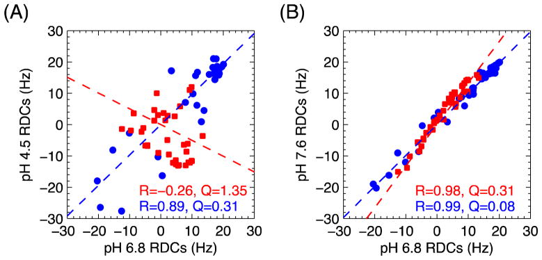
Correlation plots between the RDC data at various pH conditions for the distal (blue circles) and proximal (red squares) Ubs in K48-Ub₂. (A) RDCs at pH 6.8 versus pH 4.5. The RDCs for the distal and the proximal Ubs are completely uncorrelated (distal: R=0.89, proximal: R=−0.26), indicating a large structural difference between the two pH conditions. (B) RDCs at pH 6.8 versus pH 7.6. The good overall correlation between the RDCs (distal: R=0.99, proximal: R=0.98) suggests similarity between the structural ensembles at the two pH values. The greater than 1 slope for the proximal Ub along with the factor of ~2 greater spread of the RDC values at pH 7.6 compared to pH 6.8 suggests an increased conformational order of this Ub unit at higher pH. The dashed lines in both panels represent the corresponding regression lines. Values of the Pearson’s correlation coefficient R and the quality factor Q are indicated.

Structural interpretation of the RDCs is complicated by two issues: (i) the derived alignment tensors for the distal and proximal Ubs at each pH have significantly different principal values (Table 1), and (ii) the range of RDC values for the proximal Ub is significantly smaller than for the distal Ub, particularly at pH 4.5 and pH 6.8. These differences cannot be explained by variations in sample conditions for the proximal and distal Ub RDC data collection, since deuterium-signal splitting was identical between the two samples (see Experimental Section), and therefore suggest the existence of interdomain dynamics in K48-Ub₂.

Consequently, it is not possible to align the two Ubs with respect to each other such that a good overall fit of the combined RDCs (for both the distal and proximal Ub together) can be achieved with respect to the back-calculated RDCs from a single Ub₂ structure (Fig. 2, third column), especially at pH 4.5 and pH 6.8 (R < 0.92, Q > 0.23). Consideration of multiple conformations is therefore necessary to improve the agreement between experimental and predicted RDCs.

Interestingly, even though there is a strong correlation between the RDC data at pH 7.6 and pH 6.8, the overall spread of the proximal-Ub RDCs at pH 7.6 is slightly (1.3-fold) higher compared to that at pH 6.8 (Figs. 2 and 3B), whereas there is virtually no difference in the RDC ranges for the distal Ubs at these two pHs. This cannot be explained by a difference in the alignment medium concentration, since that would rescale the RDC values of both Ubs in Ub₂ uniformly. Also, the principal values of the alignment tensor reported by the distal and proximal Ubs are in a much closer agreement at pH 7.6 than at pH 6.8. These data point to the ability to treat (as a first approximation) the Ub₂ system as a rigid entity at pH 7.6, which prompted our attempt to construct a single conformation for the di-Ub system. The agreement between the experimental and back-calculated RDCs for this single conformation is markedly improved (R = 0.96, Q = 0.15) compared to the single conformation representations for pH 4.5 and pH 6.8, however the R and Q values are still somewhat higher than the corresponding values for the individual Ub units, indicative that certain features of the observed RDCs are not captured with a single-structure representation even at pH 7.6.

The above observations and the fact that this is a well-studied system, establish K48-Ub₂ as an excellent model system to test our sparse ensemble selection method. Therefore we applied our SES method to the RDC data, and use the results to answer several important questions: (i) whether the K48-Ub₂ takes on the same primary conformations at all pH conditions, (ii) how many major conformations are sampled, (iii) what are their associated populations, (iv) how are these populations modulated with pH, and ultimately, (v) whether these conformations can provide clues to possible mechanisms of receptors recognition by K48-Ub₂?

A Priori Analysis of RDC and SAXS Constraints for Lys48-linked Ub₂

A critical question in using experimental data as a constraint for ensemble analysis is what amount of independent information a particular type of experimental data contains, since this dictates how many independent parameters can be used to fit the data. The number of independent components is determined by the effective rank of matrix A, which can be computed a priori. Consequently, the maximum limit of the ensemble size should be constrained to no more than the effective rank of A, defined here as the number of “large” relative singular values, σ_i/σ_max (e.g. greater than 0.01).

To demonstrate the ability of such analysis to provide valuable a priori information, we compare two commonly used experimental constraints for recovering ensembles, RDCs and SAXS profiles ^21,33. We generate the A matrix from the 20000-conformers ensemble using PATI for RDC data and FoXS for SAXS data (see Experimental Section). Note that noise was included in A by scaling each row of A by the associated error estimate.

The largest twelve σ_i/σ_max values for the two generated A matrices are shown in Fig. 4A. Even before collecting any experimental data, one can see that for K48-Ub₂ the RDC matrix A contains significantly more large relative singular values than the SAXS matrix A, indicating that RDCs are more suitable for discriminating among different conformers. Figure 4A shows that using RDCs we can potentially recover a SES ensemble of up to 10 structures. By contrast, the SAXS matrix A has far fewer significant singular values, indicating that SAXS data are not as suited for accurate ensemble recovery as are RDCs, for the generated Ub₂ ensemble. There are two reasons why the SAXS matrix A has only a small effective rank: (i) the radius of gyration, is very similar for all generated Ub₂ structures (20.3±1.8 Å), and (ii) the scattering profile is bandwidth limited by the maximal interatomic distance (diameter) of the molecule, while also sampled on a very limited domain of scattering vectors (q = 0–1 Å⁻¹) ⁶⁷, meaning that the SAXS profile of any possible K48-Ub₂ ensemble contains only a small number of independent components (see also Fig. S2 and the Discussion section). In fact, our analysis showed that over 96% of the information in the SAXS profile for any Ub₂ conformer could be explained by any other conformer in the 20000-conformer ensemble. Therefore, it is difficult to select even a two-state solution for K48-Ub₂ based on SAXS data without overfitting. The theoretical observations described above guided us to use RDCs, rather than SAXS data, for SES analysis of the conformational ensemble of K48-Ub₂.

Figure 4.

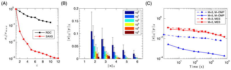
Recoverability properties of the 20000-structures RDC ensemble. (A) The σ_i/σ_max values of the largest 12 singular values of A, for RDC (black squares) and SAXS (red circles) matrices of the ensemble. (B) Average relative error in the best recovered solution, for randomly generated x with ||x||₀ non-zero values; K =10⁰,…,10⁵, from left to right. The black bars represent the standard deviation. Optimal recovery is guaranteed for ||x||₀ = 1. (C) Comparison of errors for SES and MES algorithms (blue and red symbols, respectively), as a function of computation time. No preconditioning or compression was used.

Before proceeding with an ensemble recovery, we first demonstrate our ability to recover a low-χ² solution for any sparse input vector x, generated from synthetic RDC data. Figure 4B shows that the relative error of our best recovered solution (for K >10²) is below the expected experimental error (around 5%) in RDCs. Given any set of experimentally observed RDCs coming from a 1 to 6-state ensemble, and the parameter K=10⁵, we can realistically expect to recover a “good” solution, as measured by the fit to the observed experimental data. Based on these results, we set K=10⁵ for all subsequent computations described below. At this value of K we can compute the ensemble solution in less than ten minutes on a single midrange desktop. Significant speedup was achieved for all computations described here by preconditioning χ², as detailed in Supporting Information.

Comparison to MES

We compare our Multi-OMP algorithm to the publicly available genetic-programming algorithm MES ²⁶. As the quality of the recovery can be improved by increasing the computation time in both methods, we assess the performance of MES and Multi-OMP given the same computational resources and time. The results for the 3-sized and 5-sized ensembles, using the same RDC matrix, are shown in Figure 4C. Not only does the Multi-OMP algorithm recover an order of magnitude better (in terms of relative error) solution for both M=3 and M=5, but during the same computation Multi-OMP also recovers all the solutions for ensembles of size <M. This latter feature of Multi-OMP is strategically important since we determine the optimal ensemble size based on a ℓ-curve analysis of all ensemble sizes up to the effective rank of the ab initio-generated A matrix. In contrast, the current implementation of MES requires separate computations for each value of M, resulting in a factor O(M) increase in the total computation time. The improvement in results for Multi-OMP over a genetic-programming algorithm can potentially be attributed to the better heuristic and faster recomputation of weights (see Supporting Information).

SES Analysis of RDCs for Lys48-linked Ub₂

Using our Multi-OMP algorithm, we recovered from the RDC data the best solutions for 1 to 6-state ensembles of K48-Ub₂ at all three pH conditions (Fig. 5). Since all computations are deterministic, all of the described results are entirely reproducible. For all pHs the χ² decreases monotonically as a function of the ensemble size, and for ensembles of size M=3 and above the error ε is virtually indistinguishable from ε_r, the lowest error possible when using all structures in the ensemble, and from ε_SVD, the lowest error possible when also fitting all structures and their associated alignment tensors (see Theoretical Formulation above). Since ε ≈ ε_r ≈ ε_SVD, not only did we successfully solve the SES formulation for M=3, but our 3-state SES solution is also a solution to the SVD approach.

Figure 5.

(A–B) ℓ-curve plots: (A) linear and (B) log-log plots, for M=1,…, 6 SES ensembles for K48-Ub₂ at various pH conditions. The dashed line represents both ε_SVD/L and ε_r/L, the best possible solution when fitting all 20000 columns for the SVD and ab initio predicted tensor models (but arbitrary ensemble sizes). (C) Residuals, r_i, for the x^* solutions for K48-Ub₂ RDC data at pH 4.5, 6.8, and 7.6, for M = 0 (blue), 1 (green), 2 (yellow), 3 (red). Residuals for the distal and proximal Ubs are shown on the left and right sides, respectively, of the dashed line.

We performed ℓ-curve analysis on the 1–6-sized ensembles (Figs. 5A,B). From the linear ℓ-curve plot one can see that there is only a nominal improvement in the χ² for the top M > 3 ensemble solutions. The corner point of the log-log plot suggests the selection of M = 3 as the proper ensemble size for all three pHs. Note that at pH 7.6, the contributions of 2-sized or 3-sized ensembles to reproducing the experimental RDCs are significantly smaller than at lower pH values. Furthermore, a 1-sized ensemble solution at pH 7.6 reports a better χ² value than that for a 1-sized solution at pH 4.5 or pH 6.8. These observations are in agreement with our prior assessment (see above) that, at pH 7.6, a single-conformation representation does a reasonably good job (but not entirely adequate) of reproducing the experimental RDCs (Fig. 2, third column).

The residuals between experimental and predicted RDCs for the best 1 to 3-state ensembles for all three pHs are shown in Fig. 5C. Remarkably, the agreement between the experimental RDCs and the RDCs calculated from the 3-state ensembles at each pH is as good as the agreement between the experimental and back-calculated RDCs for the individual Ub units (compare the fourth column with the first and second columns in Fig. 2). In addition, the population weights are stable with respect to experimental noise (Supporting Information).

The structures of the three ensemble members at each pH are shown in Fig. 6 (see Fig. S6 for M=1 and M=2 solutions). Importantly, at pH 4.5, all states exhibit an open Ub/Ub conformation with no obvious non-covalent contacts between the two Ub units. The populations of the 3-state ensemble at pH 4.5 are 49%, 30%, and 21%, for the three conformations. At higher pHs, we observe the emergence of a major conformation (populated at 62% at pH 6.8 and 69% at pH 7.6) that resembles the “closed” conformation of K48-Ub₂, seen previously both in crystals⁶⁸ and in solution^9,16,17,69. The increase in the population of the closed conformation is fully consistent with the better fit of RDCs to a single conformation (Fig. 2) and with our CSP data (Fig. 1). Note that the residues with significant CSPs localize to the Ub/Ub interface in the “closed” conformation¹⁷. Interestingly, the minor conformations (populations < 22%) at both pH 6.8 and pH 7.6 resemble more “open” conformations, consistent with observations from ¹⁵N relaxation data at pH 6.8 ¹⁶. All of these results are consistent with the hypothesis¹⁷ that K48-Ub₂ undergoes a population change from mainly open conformations at acidic pH, to a predominantly closed conformation at higher pH (Fig. 7). The high relative population of the closed conformation at neutral and higher pH (62–69%) is also in general agreement with prior NMR and FRET measurements ^9,11,16,17.

Figure 6.

The best overall ensemble solutions for K48-Ub₂ at pH 4.5, 6.8, and 7.6. Red coloring of the ribbon marks residues that exhibited significant spectral differences (CSPs ≥ 0.05 ppm) between the Ub₂ and the corresponding Ub monomers; the spheres (yellow) represent the side chains of the hydrophobic patch residues Leu8, Ile44, and Val70 in both Ub units. The structures are oriented such that the distal Ub is on the left and in the same orientation throughout this paper.

Figure 7.

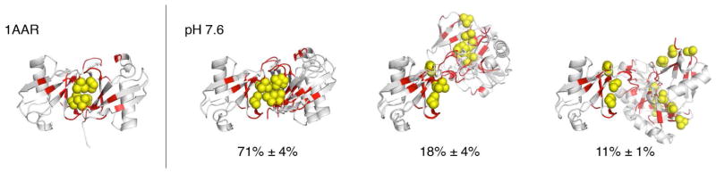
The top 3% M=3 ensemble solutions for K48-Ub₂ at pH 7.6 (the numbers show average populations) and the crystal structure (left) of the closed state of K48-Ub₂ (PDB ID 1AAR), for comparison. Red coloring of the ribbon marks residues that exhibited significant spectral differences (CSPs ≥ 0.05 ppm) between the Ub₂ and the corresponding Ub monomers; the spheres (yellow) represent the side chains of the hydrophobic patch residues Leu8, Ile44, and Val70 in both Ub units.

Alternative Ensembles that Explain Lys48-linked Ub₂ RDC Data

In addition to providing the best-χ² solution, the SES approach allows the analysis of other alternative ensembles that yield a similarly low χ². One of the advantages of the Multi -OMP computational method is that for each M-sized best ensemble we also deterministically recover K−1 best alternative solutions (see the Multi-OMP section above).

In order to visualize the structural similarity of the K−1 alternative solutions with the best solution, we analyzed all solutions within 3% of the χ² for the best solution. We then hierarchically clustered all the conformers in the best solution and all alternative solutions by 8 Å C_α-RMSD cutoff, showing only the lowest-χ² solution that comes from the same set of M clusters (see Fig. S3). The mean and standard deviation of the populations of the top 3% 3-state ensembles at pH 4.5 are [47% ± 1%, 31% ± 1%, 22% ± 1%]; at pH 6.8 are [62% ± 0%, 22% ± 0%, 16% ± 0%]; and at pH 7.6 [71% ± 4%, 18% ± 4%, 11%±1%]. The top 3% alternative solutions of the 3-state ensembles at pH 6.8 and 7.6 all have an almost identical dominant closed conformation (Fig. 7, Figs. S4, S5). Remarkably, this feature is consistently preserved even in the top 15% of the 3-state ensembles, thus demonstrating the stability of our SES results.

Comparison to Maximum Entropy Solution

Another regularization method used for ensemble selection is maximum entropy (MaxEnt) ^34,35. In contrast to the ℓ₀-norm regularization employed by SES to solve the ensemble selection problem (Eq. 6), the MaxEnt method uses relative entropy regularization to balance fit to the observed data with the divergence between the computed population weights w, and some prior distribution p,

$${\mathbf{w}}^{\ast }=\underset{\mathbf{w}}{\text{argmin}}{\chi }^2(\mathbf{w})+\lambda \sum _{j=1}^N{w}_{j}log\left(\frac{w_j}{p_j}\right),\mathrm{s}.\mathrm{t}.\sum _{j=1}^N{w}_j=1,\mathbf{w}\ge 0,$$ (8)

with λ ≥ 0 being a regularization parameter.

In order to verify that our results are mainly driven by the experimental data and not by sparsity regularization, we compared our SES results to the MaxEnt solution for all three pH conditions. MaxEnt solutions were computed using the uniform prior distribution, p_j=1/N, and λ selected using the described ℓ-curve approach (see Supporting Information for computational details and results).

Since our initial ensemble contains 20000 structures, the MaxEnt solution contains a large number of non-zero population weights. In order to interpret the results of the MaxEnt solution, we selected only the “significant” states, defined as those states with population weights greater than two standard deviations above the averaged population weight for all states. This corresponds to 559, 239, and 103 states, for pH 4.5, 6.8, and 7.6, respectively (Fig. S7). These significant states and their associated populations were aggregated together by hierarchical clustering within 4 Å Cα-RMSD. The centroids of the four most populated clusters and their associated aggregated populations are shown in Fig. 8. The displayed weights have been normalized such that the significant states’ weights add up to 1 (the absolute weights are shown in the brackets). The agreement between the experimental data and the predicted data using only the weights of the significant states is shown in Fig. S7.

Figure 8.

The results of MaxEnt analysis of the K48-Ub₂ RDC data. (A) The top four populated clusters of the significant states for the MaxEnt solution at each pH value, visually represented by their centroids, along with the clusters’ aggregated population weights. A significant state is the one that has a population of more than two standard deviations above the mean weight. The weights indicated here have been normalized such that the total weight of the significant states equals 1. The absolute (unnormalized) weights of the clusters are given in brackets. The clusters shown here include in total 268, 182, and 83 states, for pH 4.5, 6.8, and 7.6, respectively. (B) The improvement in the quality of fit as a function of the number of most populated states included. The states are sorted in descending order by their MaxEnt solution weights. The dashed line shows the best possible χ²/L value (ε_r/L) computed by minimizing Eq. 5.

From Figure 8, it is interesting to note that the MaxEnt solution does indeed capture several salient features of the K48-Ub₂ conformational ensemble. First, with increasing pH, the population of the major conformation increases from 18% to 44% for pH 6.8, and remains at 38% for pH 7.6. Only open conformations are detected for low pH, and more conformations at higher pH values resemble closed conformations of K48-Ub₂. The first two states of the MaxEnt solution are almost identical between pH 6.8 and pH 7.6 and somewhat structurally similar to each other. If combined, their populations approach the population of the major conformation in the SES solution, for their respective pHs (Fig. 6). In general, the number of states explaining the majority of experimental RDC data decreases with pH (Fig. 8B), supporting the hypothesis that K48-Ub₂ becomes more ordered at higher pH.

Unlike our SES solution, where just three representative states explain the experimental data, the first four clustered states capture only 15%, 47%, and 66% of the total population, for pH 4.5, 6.8, and 7.6, respectively, and so they cannot be interpreted directly as the four representative states (see Fig. S7). In addition, MaxEnt solution does not capture the putative closed state found in the crystal PDB structure 1AAR. Indeed, the Cα-RMSD vs. 1AAR of the MaxEnt’s major states at pH 6.8 and 7.6 is 4.8 Å, compared with 1.9 Å and 2.2 Å, respectively, for SES.

Nonetheless, it is encouraging that the maximum entropy and the SES ensemble solutions are somewhat similar at higher pH values. This suggests that the overall pattern in solutions of both methods is due to the robustness of the experimental data, rather than assumptions inherent in either method. However, three major issues hamper the MaxEnt approach: (i) the solution depends on the assumption of the prior distribution p, and therefore the ensemble generation method. A similar issue with dependence on the input ensemble arises with truncated-SVD and Tikhonov regularizations. (ii) The MaxEnt solution ensemble is difficult to interpret, requiring a further, somewhat subjective analysis, to reduce the solution to a few simple human-understandable properties ^29,34. (iii) It is difficult to adapt the method to cases when there is scaling error in the predicted data, or when some states are not in the initial ensemble, and thus the weights are not expected to add to 1.

Discussion

Here we developed a novel method for recovering multiple conformational states from a limited number of observations. We applied this method to determine, using RDC measurements, representative conformational ensembles for K48-Ub₂ as a function of pH. Our results are in full agreement with the previous observations made from entirely independent measurements, including CSPs, ¹⁵N relaxation, site-specific spin labeling ^9,16–18, and single-molecule FRET ¹¹. The fact that we were able to recover the ensembles and their associated populations based solely on a single set of RDC data suggests that sparsity regularization, known to be a powerful tool for solving numerous ill-posed problems, can also be successfully applied to the ensemble selection problem. That an entirely different method, MaxEnt, yields similar results (top populated conformers, increased conformational order at higher pH) lends further support to our findings.

Biological Relevance to Polyubiquitin Chain Recognition

The SES-derived structural ensemble of K48-Ub₂ comprises both “closed” and “open” conformations. The closed conformation, predominantly populated at pH 6.8 and 7.6, features a Ub-Ub interface formed by the hydrophobic patches of both Ub units. This interface, consistently present in all SES solutions in the top 15% clusters (Figs. S3–S5), is in full agreement with the CSPs detected in both Ub units, and resembles the Ub-Ub interface in the published (closed) structures of K48-Ub₂ (PDB IDs 1AAR, 2BGF, 3M3J) and Ub₄ (PDB IDs 2O6V, 1FJ9). Open conformations, low-populated at or near neutral pH (pH 6.8, pH 7.6), dominate the SES ensemble at acidic conditions (pH 4.5), with the closed conformation vanishing from that ensemble as its weight dropped below the detection threshold. These results are in full agreement with the experimental CSP data (Fig. 1).

Important to this analysis is the elucidation of the low-populated states at near-physiological pH, as these states structurally represent binding-competent states, whereas the major (closed) conformation does not (the Ub hydrophobic patch critical for binding is sequestered by the Ub/Ub interface). The minor conformations observed here represent low-lying excited states of K48-Ub₂, with the free-energy difference of ~1.8 RT (1.1 kcal/mol) from the major state, as determined from the differences in population between the major and minor conformations. Moreover, the fact that a single set of NMR signals was detected for each Ub in our studies indicates that the dynamic equilibrium between these states is fast on the NMR chemical-shift time scale. This then suggests that the energy barriers separating various states within the conformational ensembles derived here are such that these states are easily accessible both kinetically and thermodynamically at physiological temperatures. Importantly, in contrast to the binding-incompetent closed conformation, the hydrophobic patches in the open conformations are solvent exposed and, therefore, accessible to ligands. Thus these conformations represent binding-competent states of K48-Ub₂.

Remarkably, the inter-Ub orientations and positioning in many of the open conformations detected here resemble the bound conformations of K48-Ub₂ in complexes with various receptor proteins (see Fig. 9). For example, the UBA2 domain from the proteasomal shuttle protein hHR23a binds to K48-Ub₂ selectively and in a sandwich-like manner (Fig. 9A) ⁷⁰; this conformation is captured in one of the minor states of the (unbound) K48-Ub₂ at pH 6.8 (Fig. 6). Similar considerations apply to other known ligand-bound structures of K48-Ub₂ (Fig. 9). The insights gleaned from the structures of the minor conformers revealed here suggest that ligand recognition and binding to polyUb may employ a mechanism whereby a chain conformation predisposed for accommodating a specific ligand is selected from the available conformational ensemble; and subsequent steps might include further structural rearrangements to form the proper interfaces. The observations made here are likely to extend to other polyUb chains comprising different lysine linkages, and contribute to the understanding of how Ub chains are specifically recognized by target receptor proteins.

Figure 9.

Known ligand-bound structures of K48-Ub₂ are similar to some of the low-populated ensemble states (shown immediately to the right). The structures are oriented such that the distal Ub is on the left and has the same orientation as in all other figures in this paper. The Ub moieties are colored cyan and shown in ribbon representation, with the side chains of the hydrophobic-patch residues Leu8, Ile44, and Val70 shown as yellow spheres. The ligand is shown as white narrow ribbon and indicated for each complex.

SES Method as a General Approach to Ensemble Recovery

The SES method can be viewed as a general framework for understanding and recovering sparse conformational information from any linearly-convoluted set of experimental data or a combination thereof (e.g., RDCs and PREs). The sparsity framework allows us to avoid assuming a prior population distribution of the initial ensemble (other than sparsity), and therefore removes the dependence of the solution on the size and the sampling distribution of the initial ensemble and scaling of data, which could vary depending on the ensemble-generation and ab initio prediction methods. Such a property does not exist in maximum-entropy or energy minimization approaches.

The general applicability of a specific structural restraint, or a combination thereof, is an important theoretical question. Ideally, structural restraints should have the following two properties: (i) sensitivity, i.e. small structural alterations would result in a detectable change in experimental data, and (ii) uniqueness, i.e. no two conformers are described by the same experimental data. In terms of linear algebra, these requirements refer to the degree of correlation (orthogonality) in matrix A columns. In the ideal case, A is an orthogonal matrix where all columns are completely uncorrelated, so that the true ensemble can be unambiguously recovered, and the results are robust to experimental noise. However, in practice matrix A columns are at least partially correlated, because the number of conformers in the initial ensemble is much greater than the number of experimental observations. In that case, it still might be possible to unambiguously recover a sparse solution, but not a solution that has a large number of conformers, if small subsets of A columns are mostly uncorrelated (see restricted isometry property ⁷¹).

One can gain insight into how well different types of experimental restraints satisfy the above criteria by visualizing and comparing the pattern of values and correlation between different columns of A (as illustrated in Fig. S2). If the predicted data (divided by the experimental errors) are well spread, such that each column’s pattern is distinct, and hence not correlated, then the associated experimental data most likely have better ensemble recovery properties than those where all the columns have a similar pattern, and are correlated. See Figure S2 for the visualization of RDC, SAXS, and PRE matrices.

In our case, the columns of RDC matrix A are fairly well spread. The matrix has 10 independent components, so using RDCs as sole restraints potentially allows one to recover ensembles of size up to 10, although RDCs cannot be used to unambiguously recover larger ensembles. By contrast, the SAXS matrix A columns are highly correlated and show a similar pattern to each other (see Fig. S1). This suggests a priori that unambiguous recovery of even small ensembles using SAXS is problematic. While this observation was made for di-ubiquitin, we would expect this conclusion to hold for other molecular systems where there are no significant variations in the atom distribution between conformers. However, SAXS data can potentially supplement other experimental restraints in order to improve ensemble recovery.

Importantly, the SES formulation can be extended towards a more general concept of sparsity. In this paper we chose to interpret the experimental data in terms of the weights of individual conformational states. However, the interpretation of any particular biological system is dependent on what is biologically relevant, and one might want to seek alternative representations, such as relevant folding pathways, motion modes, or any other linear combination of individual states. Our SES approach can accommodate these alternative representations by introducing a more general formulation,

$${\mathbf{x}}^{\ast }=\underset{\mathbf{x}}{\text{argmin}}{\left|\right|\mathbf{APx}-\mathbf{y}\left|\right|}_2^2+\lambda {\left|\right|\mathbf{x}\left|\right|}_0,\mathrm{s}.\mathrm{t}.\mathbf{x}\ge 0,$$ (9)

where P is a matrix of a finite set of column vectors that map a desired sparse basis of conformational states onto probabilities of individual states, and λ is a regularization parameter that can be computed using the ℓ-curve, or some other methodology. In the study presented here, P was the identity matrix, but the columns of P can instead represent a set of possibly meaningful combinations of individual states, for example reflecting continuous motions. This allows one to extend the applicability of SES to a broader set of problems, like e.g. intrinsically disordered proteins, where a small number of conformations might not be an adequate representation. For these types of problems the flexibility of the sparsity approach over the simpler minimum ensemble selection could be important.

Finally, the SES method is a complete approach that provides:

• A method for analyzing a priori the amount of structural information that a particular set of experimental data provides.

• A problem formulation that is stable with respect to the input ensemble’s size and sampling distribution.

• A well-defined regularization technique for choosing the proper ensemble size based on fit to data.

• A robust deterministic computational method for efficiently computing a solution even for very large ensemble sizes, that can also account for errors in scaling of predicted data.

• A validation technique for checking the quality of the computed solution by comparing the errors to a lower bound determined from experimental data.

• A general model that can be adapted to individual problems by seeking various sparse solutions, not just minimum ensemble.

Our SES algorithm is simple to implement, provides a deterministic solution that requires no problem-specific tuning parameters, and has computational complexity that scales linearly with input and output ensemble sizes. Thus, SES provides entirely reproducible results that can be computed in reasonable time on individual desktops. In the case when one wishes to compute sparsest ensembles with only uniform weights, the Multi-OMP algorithm can be sped up by removing the least-squares optimization step, and introducing several other small modifications.

It is important to note that our Multi-OMP algorithm tries to improve the chance of recovery by propagating K starting points during each m iteration. Many alternative algorithms exist with different recoverability properties, however, no known algorithm can guarantee an optimal solution in a general case. It is foreseeable that, as more experimental observations are added (to y), and the initial ensemble of potential conformations is better refined, the properties of matrix A will improve such that unique and optimal sparse recovery could be guaranteed. The chance of recovery can also be potentially improved by preconditioning (Supporting Information). Realizing under what conditions the chance of recovery improves is one of the advantages of expressing this problem in terms of the M-term approximation model.

Conclusions

Here we described and demonstrated, as a proof of principle, a novel method, which we call Sparse Ensemble Selection, for determining multiple conformational states from a limited number of observations. SES recasts the problem in terms of sparse approximations, which is tied to the active research area of compressive sensing. We presented clear criteria for selecting proper ensemble sizes without overfitting the data, and described a computationally efficient deterministic algorithm that can compute these criteria in a tractable amount of time. Importantly, the method does not assume any constraints on the resulting ensemble size, individual weights, absolute scaling of data, or an error threshold, but rather determines these values as part of the computation.

We applied the SES method to elucidate the conformational ensemble of Lys48-linked Ub₂, which is the minimal structural and recognition element in longer polyUb chains. Using RDC data collected at a range of pH values from 4.5 to 7.6, we showed that our method yields structural ensembles consistent with previously published results determined by alternative methods. Our SES analysis revealed that in the low-populated conformational states of the Ub₂ the hydrophobic surface patches on both Ub units are solvent accessible, which makes these conformers ligand-binding competent. Moreover, the resemblance with the known ligand-bound structures of Lys48-linked Ub₂ suggests that some of these open conformational states are predisposed for binding to various Ub-chain receptors. These results provide an important link between the conformational properties of the polyUb signal and the possible mechanisms of its recognition by cellular receptors.

References

- 1.Boehr DD, McElheny D, Dyson HJ, Wright PE. Science. 2006;313:1638–42. doi: 10.1126/science.1130258. [DOI] [PubMed] [Google Scholar]
- 2.Korzhnev DM, Kay LE. Acc Chem Res. 2008;41:442–51. doi: 10.1021/ar700189y. [DOI] [PubMed] [Google Scholar]
- 3.Yu D, Volkov AN, Tang C. J Am Chem Soc. 2009;131:17291–7. doi: 10.1021/ja906673c. [DOI] [PubMed] [Google Scholar]
- 4.Bothe JR, Nikolova EN, Eichhorn CD, Chugh J, Hansen AL, Al-Hashimi HM. Nat Methods. 2011;8:919–31. doi: 10.1038/nmeth.1735. [DOI] [PMC free article] [PubMed] [Google Scholar]
- 5.Dethoff EA, Chugh J, Mustoe AM, Al-Hashimi HM. Nature. 2012;482:322–30. doi: 10.1038/nature10885. [DOI] [PMC free article] [PubMed] [Google Scholar]
- 6.Boehr DD, Nussinov R, Wright PE. Nat Chem Biol. 2009;5:789–96. doi: 10.1038/nchembio.232. [DOI] [PMC free article] [PubMed] [Google Scholar]
- 7.Baxter NJ, Hosszu LL, Waltho JP, Williamson MP. J Mol Biol. 1998;284:1625–39. doi: 10.1006/jmbi.1998.2265. [DOI] [PubMed] [Google Scholar]
- 8.Lipfert J, Doniach S. Annu Rev Biophys Biomol Struct. 2007;36:307–27. doi: 10.1146/annurev.biophys.36.040306.132655. [DOI] [PubMed] [Google Scholar]
- 9.Ryabov YE, Fushman D. J Am Chem Soc. 2007;129:3315–27. doi: 10.1021/ja067667r. [DOI] [PMC free article] [PubMed] [Google Scholar]
- 10.Baldwin AJ, Kay LE. Nat Chem Biol. 2009;5:808–14. doi: 10.1038/nchembio.238. [DOI] [PubMed] [Google Scholar]
- 11.Ye Y, Blaser G, Horrocks MH, Ruedas-Rama MJ, Ibrahim S, Zhukov AA, Orte A, Klenerman D, Jackson SE, Komander D. Nature. 2012;492:266–70. doi: 10.1038/nature11722. [DOI] [PMC free article] [PubMed] [Google Scholar]
- 12.Schuler B, Muller-Spath S, Soranno A, Nettels D. Methods Mol Biol. 2012;896:21–45. doi: 10.1007/978-1-4614-3704-8_2. [DOI] [PubMed] [Google Scholar]
- 13.Volkov AN, Ubbink M, van Nuland NA. J Biomol NMR. 2010;48:225–36. doi: 10.1007/s10858-010-9452-6. [DOI] [PMC free article] [PubMed] [Google Scholar]
- 14.Fushman D, Wilkinson KD. F1000 Biol Rep. 2011;3:26. doi: 10.3410/B3-26. [DOI] [PMC free article] [PubMed] [Google Scholar]
- 15.Komander D, Rape M. Annu Rev Biochem. 2012;81:203–29. doi: 10.1146/annurev-biochem-060310-170328. [DOI] [PubMed] [Google Scholar]
- 16.Ryabov Y, Fushman D. Proteins. 2006;63:787–96. doi: 10.1002/prot.20917. [DOI] [PubMed] [Google Scholar]
- 17.Varadan R, Walker O, Pickart C, Fushman D. J Mol Biol. 2002;324:637–47. doi: 10.1016/s0022-2836(02)01198-1. [DOI] [PubMed] [Google Scholar]
- 18.Lai MY, Zhang D, Laronde-Leblanc N, Fushman D. Biochim Biophys Acta. 2012;1823:2046–56. doi: 10.1016/j.bbamcr.2012.04.003. [DOI] [PMC free article] [PubMed] [Google Scholar]
- 19.Zweckstetter M, Bax A. J Am Chem Soc. 2000;122:3791–2. [Google Scholar]
- 20.Berlin K, O’Leary DP, Fushman D. J Magn Reson. 2009;201:25–33. doi: 10.1016/j.jmr.2009.07.028. [DOI] [PMC free article] [PubMed] [Google Scholar]
- 21.Huang JR, Grzesiek S. J Am Chem Soc. 2010;132:694–705. doi: 10.1021/ja907974m. [DOI] [PubMed] [Google Scholar]
- 22.Battiste JL, Wagner G. Biochemistry. 2000;39:5355–65. doi: 10.1021/bi000060h. [DOI] [PubMed] [Google Scholar]
- 23.Svergun DI, Barberato C, Koch MH. J Appl Crystallogr. 1995;28:768–773. [Google Scholar]
- 24.Forster F, Webb B, Krukenberg KA, Tsuruta H, Agard DA, Sali A. J Mol Biol. 2008;382:1089–106. doi: 10.1016/j.jmb.2008.07.074. [DOI] [PMC free article] [PubMed] [Google Scholar]
- 25.Gumerov NA, Berlin K, Fushman D, Duraiswami R. J Comput Chem. 2012;33:1981–96. doi: 10.1002/jcc.23025. [DOI] [PMC free article] [PubMed] [Google Scholar]
- 26.Pelikan M, Hura GL, Hammel M. Gen Physiol Biophys. 2009;28:174–89. doi: 10.4149/gpb_2009_02_174. [DOI] [PMC free article] [PubMed] [Google Scholar]
- 27.Petoukhov MV, Svergun DI. Biophys J. 2005;89:1237–50. doi: 10.1529/biophysj.105.064154. [DOI] [PMC free article] [PubMed] [Google Scholar]
- 28.Atilgan AR, Durell SR, Jernigan RL, Demirel MC, Keskin O, Bahar I. Biophys J. 2001;80:505–15. doi: 10.1016/S0006-3495(01)76033-X. [DOI] [PMC free article] [PubMed] [Google Scholar]
- 29.Fisher CK, Stultz CM. Curr Opin Struct Biol. 2011;21:426–31. doi: 10.1016/j.sbi.2011.04.001. [DOI] [PMC free article] [PubMed] [Google Scholar]
- 30.Schneidman-Duhovny D, Kim SJ, Sali A. BMC Struct Biol. 2012;12:17. doi: 10.1186/1472-6807-12-17. [DOI] [PMC free article] [PubMed] [Google Scholar]
- 31.Nodet G, Salmon L, Ozenne V, Meier S, Jensen MR, Blackledge M. J Am Chem Soc. 2009;131:17908–18. doi: 10.1021/ja9069024. [DOI] [PubMed] [Google Scholar]
- 32.Bertini I, Giachetti A, Luchinat C, Parigi G, Petoukhov MV, Pierattelli R, Ravera E, Svergun DI. J Am Chem Soc. 2010;132:13553–8. doi: 10.1021/ja1063923. [DOI] [PubMed] [Google Scholar]
- 33.Bernado P, Mylonas E, Petoukhov MV, Blackledge M, Svergun DI. J Am Chem Soc. 2007;129:5656–64. doi: 10.1021/ja069124n. [DOI] [PubMed] [Google Scholar]
- 34.Choy WY, Forman-Kay JD. J Mol Biol. 2001;308:1011–32. doi: 10.1006/jmbi.2001.4750. [DOI] [PubMed] [Google Scholar]
- 35.Rozycki B, Kim YC, Hummer G. Structure. 2011;19:109–16. doi: 10.1016/j.str.2010.10.006. [DOI] [PMC free article] [PubMed] [Google Scholar]
- 36.Chen Y, Campbell SL, Dokholyan NV. Biophys J. 2007;93:2300–6. doi: 10.1529/biophysj.107.104174. [DOI] [PMC free article] [PubMed] [Google Scholar]
- 37.Frank AT, Stelzer AC, Al-Hashimi HM, Andricioaei I. Nucleic Acids Res. 2009;37:3670–9. doi: 10.1093/nar/gkp156. [DOI] [PMC free article] [PubMed] [Google Scholar]
- 38.Francis DM, Rozycki B, Koveal D, Hummer G, Page R, Peti W. Nat Chem Biol. 2011;7:916–24. doi: 10.1038/nchembio.707. [DOI] [PMC free article] [PubMed] [Google Scholar]
- 39.Fisher CK, Ullman O, Stultz CM. Biophys J. 2013;104:1546–55. doi: 10.1016/j.bpj.2013.02.023. [DOI] [PMC free article] [PubMed] [Google Scholar]
- 40.Wipf DP, Rao BD. Trans Sig Proc. 2007;55:3704–3716. [Google Scholar]
- 41.Mallat S. A Wavelet Tour of Signal Processing, Third Edition: The Sparse Way. 3. Academic Press; 2008. [Google Scholar]
- 42.Elad M. Sparse and redundant representations: from theory to applications in signal and image processing. Springer; 2010. [Google Scholar]
- 43.Tjandra N, Bax A. Science. 1997;278:1111–4. doi: 10.1126/science.278.5340.1111. [DOI] [PubMed] [Google Scholar]
- 44.Fischer MW, Losonczi JA, Weaver JL, Prestegard JH. Biochemistry. 1999;38:9013–22. doi: 10.1021/bi9905213. [DOI] [PubMed] [Google Scholar]
- 45.Fushman D, Varadan R, Assfalg M, Walker O. Prog NMR Spectrosc. 2004;44:189–214. [Google Scholar]
- 46.Showalter SA, Bruschweiler R. J Am Chem Soc. 2007;129:4158–9. doi: 10.1021/ja070658d. [DOI] [PubMed] [Google Scholar]
- 47.Guerry P, Salmon L, Mollica L, Ortega Roldan JL, Markwick P, van Nuland NA, McCammon JA, Blackledge M. Angew Chem Int Ed Engl. 2013;52:3181–5. doi: 10.1002/anie.201209669. [DOI] [PubMed] [Google Scholar]
- 48.Salmon L, Bascom G, Andricioaei I, Al-Hashimi HM. J Am Chem Soc. 2013;135:5457–66. doi: 10.1021/ja400920w. [DOI] [PMC free article] [PubMed] [Google Scholar]
- 49.Berlin K, O’Leary DP, Fushman D. J Am Chem Soc. 2010;132:8961–72. doi: 10.1021/ja100447p. [DOI] [PMC free article] [PubMed] [Google Scholar]
- 50.Bruckstein AM, Donoho DL, Elad M. SIAM Rev. 2009;51:34–81. [Google Scholar]
- 51.Lawson CL, Hanson RJ. Solving Least Squares Problems. Prentice-Hall Inc; Englewood Cliffs, New Jersey: 1974. [Google Scholar]
- 52.Hansen PC, O’Leary DP. SIAM J Sci Comput. 1993;14:1487–1503. [Google Scholar]
- 53.Hansen PC. Numer Algor. 2007;46:189–194. [Google Scholar]
- 54.Natarajan BK. SIAM J Comput. 1995;24:227–234. [Google Scholar]
- 55.Davis G, Mallat S, Avellaneda M. Constr Approx. 1997;13:57–98. [Google Scholar]
- 56.Pati YC, Rezaiifar R, Krishnaprasad PS. Proc 27th Annual Asilomar Conf on Signals, Systems, and Computers; IEEE. 1993. pp. 40–44. [Google Scholar]
- 57.Bruckstein AM, Elad M, Zibulevsky M. IEEE Trans Inf Theor. 2008;54:4813–4820. [Google Scholar]
- 58.Needell D, Vershynin R. Found Comput Math. 2009;9:317–334. [Google Scholar]
- 59.Blumensath T, Davies ME. Trans Sig Proc. 2009;57:4333–4346. [Google Scholar]
- 60.Delaglio F, Grzesiek S, Vuister GW, Zhu G, Pfeifer J, Bax A. J Biomol NMR. 1995;6:277–93. doi: 10.1007/BF00197809. [DOI] [PubMed] [Google Scholar]
- 61.Goddard TD, Kneller DG. SPARKY3. University of California; San Francisco: [Google Scholar]
- 62.Ruckert M, Otting G. J Am Chem Soc. 2000;122:7793–7797. [Google Scholar]
- 63.Clore GM, Garrett DS. J Am Chem Soc. 1999;121:9008–12. [Google Scholar]
- 64.LaValle SM, Kuffner JJJ. Algorithmic and Computational Robotics: New Directions. 2000:293–308. [Google Scholar]
- 65.Gray JJ, Moughon S, Wang C, Schueler-Furman O, Kuhlman B, Rohl CA, Baker D. J Mol Biol. 2003;331:281–99. doi: 10.1016/s0022-2836(03)00670-3. [DOI] [PubMed] [Google Scholar]
- 66.Schneidman-Duhovny D, Hammel M, Tainer J, Sali A. Biophys J. 2013;105:962–74. doi: 10.1016/j.bpj.2013.07.020. [DOI] [PMC free article] [PubMed] [Google Scholar]
- 67.Koch MH, Vachette P, Svergun DI. Q Rev Biophys. 2003;36:147–227. doi: 10.1017/s0033583503003871. [DOI] [PubMed] [Google Scholar]
- 68.Cook WJ, Jeffrey LC, Carson M, Chen Z, Pickart CM. J Biol Chem. 1992;267:16467–71. doi: 10.2210/pdb1aar/pdb. [DOI] [PubMed] [Google Scholar]
- 69.van Dijk AD, Fushman D, Bonvin AM. Proteins. 2005;60:367–81. doi: 10.1002/prot.20476. [DOI] [PubMed] [Google Scholar]
- 70.Varadan R, Assfalg M, Raasi S, Pickart C, Fushman D. Mol Cell. 2005;18:687–98. doi: 10.1016/j.molcel.2005.05.013. [DOI] [PubMed] [Google Scholar]
- 71.Candes EJ. C R Seances Acad Sci, Ser A. 2008;346:589–592. [Google Scholar]
Associated Data
This section collects any data citations, data availability statements, or supplementary materials included in this article.