Statistical Approach to Protein Quantification

Abstract

A major goal in proteomics is the comprehensive and accurate description of a proteome. This task includes not only the identification of proteins in a sample, but also the accurate quantification of their abundance. Although mass spectrometry typically provides information on peptide identity and abundance in a sample, it does not directly measure the concentration of the corresponding proteins. Specifically, most mass-spectrometry-based approaches (e.g. shotgun proteomics or selected reaction monitoring) allow one to quantify peptides using chromatographic peak intensities or spectral counting information. Ultimately, based on these measurements, one wants to infer the concentrations of the corresponding proteins. Inferring properties of the proteins based on experimental peptide evidence is often a complex problem because of the ambiguity of peptide assignments and different chemical properties of the peptides that affect the observed concentrations.

We present SCAMPI, a novel generic and statistically sound framework for computing protein abundance scores based on quantified peptides. In contrast to most previous approaches, our model explicitly includes information from shared peptides to improve protein quantitation, especially in eukaryotes with many homologous sequences. The model accounts for uncertainty in the input data, leading to statistical prediction intervals for the protein scores. Furthermore, peptides with extreme abundances can be reassessed and classified as either regular data points or actual outliers.

We used the proposed model with several datasets and compared its performance to that of other, previously used approaches for protein quantification in bottom-up mass spectrometry.

The comprehensive and quantitative analysis of proteins expressed in various organisms, tissues, or cell lines provides important insights into systems biology that cannot be inferred with the use of genomics or transcriptomics approaches (3). Although protein identification remains an important topic of ongoing research, the focus has moved to quantification in recent years. Not only is it important to know which proteins are present in a sample, but the abundance of these molecules is also of major interest. For instance, one would like to be able to identify which are the most or least abundant proteins in a sample, or to compare the concentration of the same protein in two samples taken under different biological conditions. In medical sciences, for example, biomarkers can be used to distinguish healthy from ill patients or allow one to monitor the efficiency of a treatment by comparing a molecule's concentration before and after therapy (4).

Most methods for analyzing mass spectrometry (MS)-based¹ proteomics data rely on a sequential approach: first identification and then quantification of the peptides and proteins in a sample (5, 6). Peptide identification is based on finding the peptide sequences corresponding to the measured spectra, and it has been intensely studied. A wide range of solutions have been proposed, for example, in Refs. 7–10. A recent review of the main approaches can be found in Ref. 11. The inference of protein abundance relies on quantitative information about the corresponding peptides, usually either chromatographic peak intensities (ion-currents) or spectral counts (the number of recorded MS/MS spectra). Thus, the peptides are usually quantified first, and then this knowledge is transferred to the protein level.

The protein inference problem (12) consists of deciding which protein sequences are present in a sample based on the set of identified peptide sequences.² It has been addressed in many works, including Ref. 10 and Refs. 13–19. The methods vary according to the underlying model, the implied independence assumptions, and the way of handling shared peptides (which match to several protein sequences and are also called degenerate (or degenerated) peptides).

Many different approaches for protein quantification have been published in the past few years. Some of them are applied directly to raw data (e.g. SuperHirn (20), MaxQuant (10), Progenesis (21), and OpenMS (22)), primarily to obtain quantitative information in the form of intensities or spectral counts for the peptides. Other tools are exclusively designed to combine or transform peptide abundances into quantitative data at the protein level (e.g. emPAI (23), APEX (24), mSCI (25), TOPn (2), MSstats (26), SI_N (27), and SRMstats (28)). Further differences between the approaches arise from their use of peak intensities or spectral counts as measures for the peptide abundance, whether they specialize in absolute or relative quantification, which mass spectrometric technique is used (discovery-driven, directed or targeted MS (29)) and which, if any, isotopic labeling of the peptides is supported. Most publications proposing a procedure based on peptide intensities actually provide an elaborate solution for quantifying peptides (allowing one to combine replicates or normalize the data) but rely on a very simple averaging approach to combine these scores into estimates for protein concentrations. Notably, none of the methods mentioned above—including methods based on spectral counts—take full advantage of the information withheld in shared peptides. Instead, the degenerate peptides are grouped, reassigned to single proteins, or even discarded in order to derive a simple solution to the identification and quantification of proteins. Studies focusing on the inclusion of shared peptides in the protein quantification process include Refs. 30–33.

Although shared peptides make the protein quantification problem more difficult and can introduce errors in the estimates when not handled properly (30), they also hold essential information. Being able to use this additional knowledge is of great importance, especially when working with higher eukaryotes. In such organisms it is difficult to observe enough unique peptides per protein (peptides matching to a single protein) for quantification (32). Furthermore, a lot of valuable information is lost when shared peptides or indistinguishable proteins are discarded or grouped.

Here we present SCAMPI, a statistical model for protein quantification. In contrast to most existing approaches, SCAMPI includes quantitative information from shared peptides. Furthermore, it is generic in the sense that (i) input can come from various experiments (e.g. SRM or shotgun, isotope-labeled or label-free) and (ii) the choice of method used to compute the peptide abundances is left to the user. In addition, an abundance score is computed for each protein matching to at least one experimentally observed peptide (no grouping). The implemented model holds several parameters that are trained on the dataset, allowing it to be adapted to different types of input/instrumentation/experiments. The underlying assumptions are clearly stated, and a proper statistical framework is used. In comparison to models such as those described in Refs. 30–32, SCAMPI offers a novel approach involving a probabilistic framework and generic formulation. In contrast to previous models handling shared peptides, SCAMPI readily provides a prediction interval for each protein abundance score and allows one to reassess the peptide abundances.

The “Results” section of this paper describes the application of SCAMPI to three datasets and compares its performance to that of some previously used protein quantification methods, namely, TOPn (2) and MaxQuant (10), which are briefly discussed below. The examples shown rely on intensity-based peptide abundances. Applications to spectral count data might be possible, but this would require further investigation.

TOPn

This approach quantifies a protein based on its identified unique peptides exhibiting the most intense mass spectrometry response (best flyer peptides). TOPn is based on the assumption that the peptide specific MS response of the best flyer peptides is approximately constant throughout the whole proteome. The validity of this assumption was empirically tested and demonstrated for the first time by Silva et al. (2) and was applied at a proteome-wide scale by Malmström et al. (34). Additional information contained in shared peptides is disregarded by TOPn. The approach attempts to predict the protein concentration by averaging the peptide concentration of its n most abundant peptides, with n often set at 3. If this requirement of having three unique peptides quantified for each protein were applied strictly, TOP3 would be able to estimate concentrations for only a small fraction of the proteins in samples from higher eukaryotes (with many similar protein sequences). In practice, however, proteins are often quantified even if they have only one or two unique peptides.

MaxQuant

This method was originally designed for relative protein quantification based on peptide intensities. MaxQuant allows one to align, normalize, and quantify spectra over multiple peptides and then combines these results to compute relative protein abundances. The issue of shared peptides is avoided through the grouping of indistinguishable proteins.

Besides relative comparisons of protein quantities, our method can also be used for absolute quantification through the use of carefully selected anchor proteins (e.g. 1, 34–36). Absolute values are required in order to determine stoichiometries of protein complexes and to facilitate mathematical modeling, for example, of cell signaling. Absolute protein quantification is also important for many questions in molecular biology and medical sciences, for example, when one would like to compare results obtained on different platforms, with different settings, or across various species.

An additional feature provided by our model is the possibility of using the computed protein abundance scores to reassess the peptide input scores. Dost et al. (32) also briefly mention this option as an advantage of using approaches including shared peptides. As mentioned above, shared peptides hold additional information and thus allow one to discover discrepancies in the input data that might be missed when focusing only on unique peptides.

The model is fully described in the section “Materials and Methods,” and some of its properties are further highlighted in the “Discussion.” Its performance with several datasets is evaluated in the “Results” section and compared with the results obtained with other protein quantification approaches.

MATERIALS AND METHODS

Our proposed model is designed to estimate protein abundance scores based on experimental quantitation knowledge gained at the peptide level via MS-based approaches (e.g. shotgun proteomics or SRM). The model is applied to one sample (one biological replicate) at a time. The input data consist of n identified peptide sequences and their m matching protein sequences in a given sample. Choices such as how to handle charge states, modifications, or semitryptic peptides are left to the user (see “Workflow and Input Data” in the supplemental material for details).

For each peptide, the model requires an input score U_i (i = 1, …, n) that is assumed to be proportional to the peptide's abundance. As values for U_i, one can, for example, use a (log-transformed) measurement of the total ion current (intensity) of a peptide. The aim of the model is to infer the abundance C_j for each protein matching to at least one experimentally quantified peptide (j = 1, …, m). As an underlying data structure, the model uses a bipartite graph, with one set of nodes representing the peptides and the other one the proteins. There is an edge between two nodes if and only if the peptide sequence is part of the protein sequence (inclusion). The graph is composed of many connected components (also called subgraphs) that are referred to as cc_r (r = 1, …, R). Each connected component holds n_r peptides and m_r proteins. Fig. 1 exemplifies the notation.

Fig. 1.

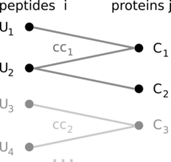
Bipartite graph with experimentally identified peptide (left-hand side) and matching protein sequences. There is an edge between a peptide and a protein if and only if the peptide sequence occurs exactly in the protein sequence. Each peptide i (i = 1, …, n) has a score U_i that is assumed to be proportional to its abundance. The aim of the model is to infer the concentration C_j for each protein in the graph (j = 1, …, m). The graph is composed of many subgraphs, or connected components, which are referred to as cc_r (r = 1, …, R). Each connected component holds n_r peptides and m_r proteins.

The data on peptide level, U_i, are known from experiments. The protein abundance C_j is a latent variable. The main goal of the presented approach is to compute estimates Ĉ_j. To address this aim, we designed a model for U_i, from which we will later infer the estimates Ĉ_j:

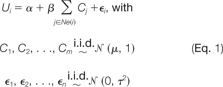where Ne(i) denotes the set of proteins having a common edge with peptide i (neighbors of i) and ϵ₁, …, ϵ_n are independent of C₁, …, C_m. The parameters α, β, μ, and τ are unknown and will be estimated from the data. Briefly, we assume that U_i depends linearly on the abundance of the neighboring proteins. Furthermore, we include an intercept α that allows us to take into account a possible shift in the measured values for different platforms and/or organisms. Eventually, the model will contain an error term to account for measurement and modeling errors. Note that $C_j\stackrel{i.i.d.}{{\displaystyle \sim }}$ Ν (μ, 1) provides the prior value for each protein abundance. The posterior distributions, used for statistical inference, are different for each protein. In other words, all proteins C_j are, a priori, treated equally with the same prior distribution Ν (μ, 1). The posterior distribution is obtained by updating this prior assumption using the data about peptides. Prior distributions with an i.i.d. structure (as here) are widely used in Bayesian statistics (and frequentist statistics in connection with random effects models). We further note that the whole dataset is used for the training of the parameters, even if abundance predictions are required for only a small subset of the proteins.

Working on a bipartite graph naturally leads to some Markovian-type assumptions (37):

Hence, dependences among peptides are exclusively due to their common proteins. In addition, the model assumes that only neighboring proteins matter in the (conditional) distribution for the peptides (see also Ref. 16).

For better readability, we introduce the following notations.

• U^(r) is the vector of all U_i for peptides belonging to the rth connected component (n_r × 1).

• 1^(r) = (1, …, 1)^T (for the connected component r, this is an n_r × 1 vector).

• The n_r × n_r matrix D^(r) gives information about the connectivity in the connected component r:

  • D_ii^(r) = number of proteins sharing an edge with peptide i.
  • D_ik^(r) = number of proteins sharing an edge with peptide i and peptide k.

Given the peptide scores, an estimate of the abundance of a protein j in connected component r is Ĉ_j = E [C_j|U^(r)]. With multivariate analysis theory (see pp. 33–34 in Ref. 38) and using the Markovian assumption (Equation 2), this can be rewritten as

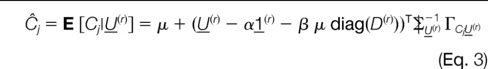The variance of the protein abundance estimates given the peptide scores U_i can be computed as

Thereby, the covariances between the peptide scores (Σ|) and between the peptide and protein scores (Γ) are defined as follows (see “Covariances” in the supplemental material for details):

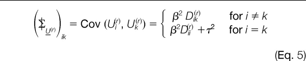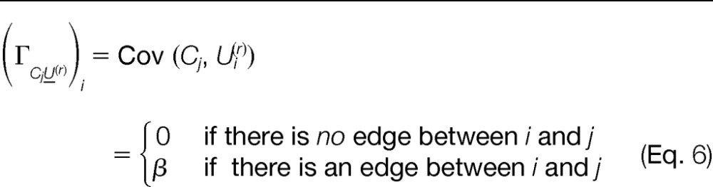The covariances between different connected components are all zero.

Note the choice of a variance of 1 for the distribution for the protein scores in Equation 1. Using an additional parameter—say, ${\underset{¯}{C}}_j\stackrel{i.i.d.}{{\displaystyle \sim }}$ Ν (μ, σ²), would lead to a nonidentifiable model. In fact, any value set for σ can be compensated by reparametrizing β and μ. Hence, the model as presented in Equation 1 with the four parameters α, β, μ, and τ is retained. Two approaches for estimating the parameters from data are discussed in the section “Parameter Estimation.”

An important advantage of a model-based approach such as SCAMPI is the possibility of estimating the accuracy of the predicted scores.

where z = 1.96 for a 95% prediction interval. In the presence of anchor proteins, one is interested in using this additional information to transform the computed scores Ĉ_j into estimates of the absolute protein concentration C̃. We do this with a linear transformation C̃_j = â + b̂ Ĉ_j for all proteins in the sample. The parameters â and b̂ are estimated for the subset of anchor proteins via a linear regression model, C_anchor = log₁₀(concentration_anchor) = a + b Ĉ_anchor + ε, where ε is a mean zero error term. The 95% prediction intervals for C̃_j are then given by C̃_j ± 1.96b̂ $\sqrt{\text{Var}\left({\widehat{C}}_j|{\underset{¯}{U}}^{\left(r\right)}\right)}$. Note that the uncertainty of the parameter estimates is ignored when computing these intervals. Furthermore, note that the anchor proteins should be chosen so as to cover a broad dynamic range, and one should only trust predictions lying in this interval. There is no reason to assume that the fitted linear model is suitable for predicting much less or more abundant proteins.

Peptide Reassessment

Consider the peptide quantities that are explicitly modeled in Equation 1. Fig. 2 describes a hypothetical example of a situation in which some peptide abundances appear to have, at first glance, surprisingly high values. If a protein quantification model can handle shared peptides, it should be able to identify which of these high peptide abundances correspond to real outliers and which ones are due to the aggregation of several proteins.

Fig. 2.

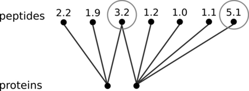
Hypothetical example to illustrate the idea behind SCAMPI's peptide reassessment step. The given peptide scores could be any abundance measure (e.g. logarithmized peak intensities). At first glance, there seem to be discrepancies in the measurements for the circled peptides. However, considering the graph structure, only the peptide with a value of 5.1 cannot be explained and is thus a “real” outlier. Indeed, the value of 3.2 can be explained by a contribution from both proteins. An example of a real connected component is discussed in the supplemental material (“Directed MS Human Data”).

If the protein abundances were known, one could compute the peptide quantities with the model and check whether the predicted and measured values matched. In most cases the true protein abundances are not known, but the predicted values Ĉ can be used to compute estimates of the peptide quantities (see Equation 8). Comparing these estimates to the original values allows us to identify outliers in the peptide measurements.

Of course, one should not use a peptide quantity to estimate a protein abundance and then reuse this estimate to predict this same peptide's abundance; this would lead to overfitting and potentially overly optimistic results. Instead, the expected value for the abundance of peptide i given all other peptide measurements ({U_k\i}) is computed (see “Reassessing Peptide Abundances” in the supplemental material for details).

Hence, to predict the quantity of peptide i, estimates of the protein abundances (see Equation 3, but adapted to {U_k\i}) computed by using all peptide intensities except the ith one are used. The estimated Û_i values can then be compared with the measured U_i values. For connected components holding a single peptide, the formula simplifies to Û_i = α + βμD_ii. Note that although there are no further peptides in the connected component, U_i can still be approximated thanks to the parameters trained on the whole dataset and the number of neighboring proteins to peptide i. “Selecting Outliers in the Measured Peptides” in the supplemental material provides details about the selection of the outliers.

Outliers may be observed in the peptide data for several reasons, including measurement errors, incomplete database searches, missed cleavages, and modified sequences. Being able to automatically compile a list of peptide outliers might help one to gain a better understanding of the data. The selected outlying peptides can then be validated individually, for example, by finding reasons for their peculiar abundance scores.

Parameter Estimation

A classical approach for estimating the unknown parameters (α, β, μ, and τ) in our model is the use of maximum likelihood estimation (MLE). From the model in Equation 1, it follows that

and the density function of U^(r) is given by

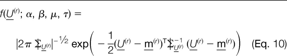Maximizing the likelihood is equivalent to minimizing the negative log-likelihood, which is given by

where the independence among different connected components (see Equation 2) has been invoked. Minimizing the function in Equation 11 with respect to the four parameters yields estimates for α, β, μ, and τ. Positivity constraints are used for β, μ, and τ.

Although MLE is typically optimal from an asymptotic point of view (e.g. 39), the computations are rather expensive because of the involved numerical optimization over a four-dimensional space.

The sample size (i.e. the number of peptides in the dataset) is typically large (relative to the number of parameters in the model), and thus efficiency issues regarding the estimator are negligible in comparison to modeling errors. Thus, as an alternative to the MLE, a method of moments approach that needs much less computation time and leads to results similar to those of the MLE for the tested datasets (see “Results”) is suggested. This second method relies on least squares estimations on the elements of the covariance matrix Σ|. Henceforth, we refer to this parameter estimation approach as indirect least squares estimation (ILSE). In detail, several steps are needed.

1. From Equation 1, it is known that E [U_i] = α + βμD_ii. Fitting a linear regression model with the peptide intensity U as a response variable and the number of neighboring proteins diag(D) as a predictor variable (U ∼ diag(D)) provides the estimates α̂ (intercept) and $\widehat{\beta \mu }$ (slope).

2. Compute the sample covariance matrix estimated for each connected component cc_r.

   
3. Compare the off-diagonal elements of the sample covariance matrix with the parametric version given in Equation 5. Minimize the sum of squared errors.

   

   with respect to β². This allows us to compute the estimated β̂, as well as μ̂ (from the previously computed $\widehat{\beta \mu }$ (step 1)).
4. Similarly, working on the diagonal elements of Σ| and plugging in β̂ (step 3) yields the estimate τ̂ by minimizing the sum of squared errors

   

   with respect to τ².

The solutions to the minimization problems in Equations 13 and 14 can be written in closed form (see “ILSE Parameter Estimates” in the supplemental material). Thus, no numerical optimization is required, and the estimates can be computed quickly even for large datasets.

The two approaches can also be combined by using the estimates computed via ILSE as starting values for the numerical optimization performed in the MLE approach.

Note that if a dataset does not hold any shared peptides, the parameters are nonidentifiable. The estimates Ĉ_j in Equation 3 and Û_i in Equation 8 are still well defined, though. Whereas no adjustment is required for the MLE approach, ILSE is not applicable directly as described above. As a workaround, μ̂ is set to zero in such situations; α̂ is then the average of all input peptide abundance scores, and β̂ and τ̂ are computed as described in Equations 13 and 14.

Relative Quantification

It is often of interest to compare the abundance of a protein under two conditions. For such a comparison, SCAMPI can be used to compute the protein abundance scores on each sample separately. A quantile-quantile plot of the protein abundance scores can be used to assess whether the two score distributions are comparable (e.g. comparable median and quartiles of the two conditions). The score differences can then be assessed to find proteins undergoing particularly high changes in abundance: D_j = Ĉ_j^{condition 2}−Ĉ_j^{condition 1}. Ideally, one would have several biological replicates in each condition to make sure one could distinguish the effect due to the condition from the variability within the condition.

Typical Workflow

The model has been implemented in R (40) (see “Implementation”) and is available in the R package protiq (41) on the Comprehensive R Archive Network (CRAN).

The following steps are required in order to run SCAMPI.

1. Prepare the input data (three input tables; see “Workflow and Input Data” in the supplemental material for details):

   1. Data frame of quantified peptides: each row corresponds to one peptide and includes the sequence, as well as a score related to the peptide's abundance (U). Note that each peptide should occur only once in this table. It is up to the user to decide how to aggregate the scores in the case of multiple features matching the same peptide or, for example, whether sequences with different charge states should be combined in a single peptide or treated as separate instances. The user also has to decide how to handle modifications and semitryptic peptides at this stage.
   2. Data frame of matching proteins: each row corresponds to one protein and includes the identifier or sequence of the protein. Note that this table should not contain the same protein sequence several times. This requires particular attention when a sequence is described by several accession numbers.
   3. Data frame providing information as to which peptide matches which protein. Each row of this table defines one edge of the bipartite graph.

2. Estimate the model parameters (with either the MLE or the ILSE approach).

3. Compute the protein abundance scores Ĉ (Equation 3 with estimated parameters from step 2).

4. Optionally, compute peptide intensities given the estimates Ĉ (Equation 8 with estimated parameters from step 2) and compare Û to the input values U. Identify outliers.

5. Optionally, reevaluate steps 3 and 4 after having removed the outliers and updated the bipartite graph.

The workflow is depicted in the supplemental material (“Workflow and Input Data”).

Note that the model does not provide methods for combining measurements from, for example, different technical replicates or charge states. The user is expected to perform these adjustments prior to applying the protein quantification model, for example, by running one of the peptide quantification tools mentioned in the Introduction. As examples, descriptions of how the datasets presented in the “Results” section have been prepared are provided in the supplemental material (“Input Data Preparation for SCAMPI”).

Overview of the Assumptions

It is important to keep the modeling assumptions in mind.

1. Peptide abundances are modeled as random quantities, allowing one to account for measurement uncertainty and modeling errors.

2. There is a Markovian-type assumption in Equation 2 (see also Ref. 16):

   1. Connected components are independent.
   2. Peptides are independent given the matching proteins. In other words, dependences among peptides are exclusively due to their common proteins.
   3. Only neighboring proteins influence the conditional distribution of the peptides.

3. The error terms ϵ_i are i.i.d. and follow a normal distribution.

4. Statistical prior distribution for the protein abundances C_j: they are i.i.d. and follow a normal distribution.

5. ϵ₁, …, ϵ_n are independent of C₁, …, C_m.

In practice, only assumption 3 is easily verifiable, for example, by using a normal plot for residuals. However, Markovian-type assumptions for graphs are often used in similar problems and allow one to account for some dependence (among and between peptides and proteins) while rendering the problem computable. Regarding the normality assumption for the protein abundances, E [C_j|U] is linear for U_i's in the Gaussian case. In the non-Gaussian case, E [C_j|U] might be nonlinear, but the formula from the Gaussian case still leads to the best linear approximation for the estimates of Ĉ_j.

RESULTS

The proposed model has been tested on several datasets and compared with the previously used protein quantification approaches TOPn (2) and MaxQuant (10). The presented datasets include (i) mixtures with added AQUA peptides (1) used to experimentally quantify a subset of the proteins (see “SRM Experiment on Leptospira interrogans” (36) and “Directed MS Human Data” (42)) and (ii) a human SILAC-labeled proteomics experiment without a known ground truth (see “SILAC-labeled Human Shotgun Proteomics Data”). The authors of each dataset provided the input data required for running SCAMPI. The data, prepared to be used for analysis with SCAMPI, are provided in the supplemental material.

The protein concentration scores computed by SCAMPI were compared with the ground truth (if available) and to the results obtained with quantification tools used by the authors of the data. As performance measures for the models, the Pearson correlation coefficient R and Spearman's rank correlation coefficient ρ are reported. A table summarizing the size of each dataset and the computation times is provided in the supplemental material (“Computation Times”).

The provided examples show that SCAMPI performed similarly to other, previously proposed quantification tools. In addition, they highlight some advantages of SCAMPI relative to other tools.

SRM Experiment on Leptospira interrogans

In a recent paper about label-free absolute protein abundance estimation using SRM, Ludwig et al. published experimental data from cellular protein lysates of Leptospira interrogans proteins. The measurements were based on SRM and the best flyer methodology. Experimental details are provided in Ref. 36, and the data are published in the supplemental material for that article. The sample contained 39 proteins, of which 16 were used as anchor proteins, and their concentration was accurately determined with AQUA peptides (1). The performance of SCAMPI is compared with TOP3 on the 16 anchor proteins for the control mixture. The complete dataset held 151 peptides uniquely matching one of the 39 proteins, and the bipartite graph held 39 connected components. Thus, the dataset did not contain any shared peptides. Although the new model is primarily designed to solve more complicated problems with (many) shared peptides, this first test dataset allowed us to give proof of principle that the presented model also works in simpler situations. Details about the preparation of the input data for SCAMPI are provided in the supplemental material (“Input Data Preparation for SCAMPI”). The estimated parameter values are also provided (“Parameter Estimates”).

SCAMPI's results were compared with the output from the TOP3 (2) approach. A TOP3 abundance score was computed for each protein with at least one matching unique peptide. The estimates of the protein concentrations are shown in Fig. 3. Panel A shows the results obtained with SCAMPI when using the ILSE parameter estimates. The error bars correspond to the 95% prediction intervals for the computed protein scores. Panel B shows the outcome for the TOP3 approach. The correlation coefficients obtained with the different approaches are very similar.

Fig. 3.

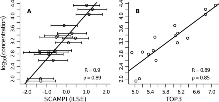
L. interrogans dataset—protein abundance estimates for the 16 anchor proteins. A, results for SCAMPI (using ILSE parameter estimates). The error bars correspond to the 95% prediction intervals. B, outcome for the TOP3 approach. The correlation coefficients in the two panels are very similar. Performance measures: R and ρ indicate the Pearson and Spearman's rank correlation coefficients, respectively. Note that the scale on the x-axis is different in the two panels. The range of the computed scores depends on the underlying model. We cannot compare the scores from SCAMPI and from TOP3 directly, but we can look at correlations with a reference score, as presented in this figure.

The results obtained with SCAMPI when using the MLE parameter estimates were very similar to the ones presented above. For the sake of completeness, the resulting plots are provided in the supplemental material, together with some Bland–Altman (43) and diagnostic plots.

Directed MS Human Data

Beck et al. have provided a quantitative analysis for the human tissue culture cell line U2OS based on directed MS experiments. Some AQUA peptides (1) were spiked into the mixture to allow the absolute quantification of 53 proteins over a wide range of concentrations. See Ref. 42 for experimental details.

Beck et al. provided the Progenesis (21) peptide quantification scores for the control mixture. Details about the preparation of the input data for SCAMPI are provided in the supplemental material (“Input Data Preparation for SCAMPI”). The dataset held quantification information for 49,190 peptides, about 6% of which were shared by at least two different protein sequences. The graph included data for 6257 proteins and 54,720 edges and could be split into 4984 connected components. The estimated parameter values for SCAMPI are reported in the supplemental material (“Parameter Estimates”). The performance was assessed on the 42 anchor proteins for which experimental data were available at the peptide level (see “Input Data Preparation for SCAMPI” in the supplemental material for details).

The performance of SCAMPI is compared with that of the TOP3 approach (2) in Fig. 4. A TOP3 abundance score was computed for each protein with at least one matching unique peptide. The error bars in panel A correspond to the 95% prediction intervals for the computed protein scores. The reported correlation scores were similar for the different approaches. TOP3 slightly outperformed SCAMPI in terms of both ρ and R. However, note that although the dataset held about 7 peptides per protein on average, a strict TOP3 approach (quantifying only proteins with at least three quantified matching unique peptides) would not have been able to predict the abundance of each protein in the dataset. Thus, some of the reported protein abundances computed by TOP3 relied on the values of one or two measured peptides only. In contrast, SCAMPI uses additional knowledge from shared peptides (if available) and from the whole dataset (through the estimated parameters) to provide an abundance score for each protein. Moreover, SCAMPI, unlike TOP3, also provides the prediction error for each protein.

Fig. 4.

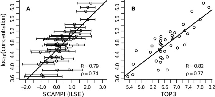
Directed MS human dataset—protein abundance estimates for the 42 anchor proteins. SCAMPI (ILSE parameter estimate) in A is compared with the TOP3 approach in B. The performance scores are similar in the two subfigures. The error bars in A correspond to the 95% prediction intervals. Performance measures: R and ρ indicate the Pearson and Spearman's rank correlation coefficients, respectively. Note that the scale on the x-axis is different in the two panels. The range of the computed scores depends on the underlying model. We cannot compare the scores from SCAMPI and from TOP3 directly, but we can look at correlations with a reference score, as presented in this figure.

The results obtained with SCAMPI when using the MLE parameter estimates were very similar to the ones presented above. For the sake of completeness, the resulting plots are provided in the supplemental material, together with some Bland–Altman (43) and diagnostic plots.

Finally, the predicted concentrations for all proteins in the dataset were compared with the results published in Ref. 42. The latter predictions were computed with SSID/MW, a method based on spectral counting (see the supplemental material for Ref. 42 for more information). Comparing the SSID/MW results to the protein concentrations predicted by SCAMPI yielded a Pearson correlation coefficient of 0.81 and a Spearman's rank correlation coefficient of 0.74. The comparison was based on 1741 proteins that were quantified by both models and which had values in the range covered by the anchor proteins.

SILAC-labeled Human Shotgun Proteomics Data

This dataset came from a human acute myeloid leukemia cell line (KG1a cells). Cells were grown in SILAC media containing either light or heavy isotope. The cells labeled with heavy isotope were treated with proteasome inhibitor. The untreated cells (control) were grown in the presence of the light isotope. Details about the experimental procedure are provided in the supplemental material (“Materials and Methods for the SILAC Dataset”).

The MaxQuant (10) peptide quantification results for the cytoplasmic fraction were used as input for SCAMPI. The measurements for the control and treated conditions were analyzed separately. Details about the preparation of the input data for SCAMPI are provided in the supplemental material (“Input Data Preparation for SCAMPI”).

The underlying graph used for both samples was slightly different, because there were a few peptides (fewer than 20) that could be quantified in only one of the two samples. For the control mixture, the graph held 30,323 peptides, 3892 proteins, and 38,019 edges organized in 2659 connected components. In the treated case, the graph held 30,326 peptides, 3890 proteins, and 38,025 edges organized in 2658 connected components. In both conditions, about 17% of the peptides were shared (i.e. matched to more than one protein sequence). The estimated parameter values for SCAMPI are reported in the supplemental material (“Parameter Estimates”).

Although there was no known ground truth for this dataset, it is an interesting example (given the high percentage of shared peptides) of how SCAMPI can be used to analyze relative protein abundance. Furthermore, it emphasizes SCAMPI's flexibility regarding the type of peptide-level input it can handle (in this case, peak intensities computed by MaxQuant). This dataset was used primarily to show how SCAMPI can be used to identify differentially abundant proteins and to explore a dataset by reassessing peptide scores. In addition, it illustrates how running SCAMPI recursively can improve the predictions. The resulting parameter estimates from ILSE and MLE were again very similar. The ILSE results are discussed here. The plots for the MLE estimations are provided in the supplemental material.

Fig. 5 shows the obtained protein abundance score distributions for both conditions. The quantile-quantile plot in Fig. 5C confirms that direct comparisons between computed scores from the two conditions are reasonable. Hence, in order to investigate whether the abundance of some proteins changed between the two conditions, the score difference D_j = Ĉ_j^treated − Ĉ_j^control was analyzed. For this comparison, only proteins that could be quantified in both conditions were used (i.e. not being measured was not treated as being absent from the sample). The empirical distribution of the abundance changes D_j is shown in Fig. 6. Proteins with particularly high score differences are highlighted. An interquartile-based discrimination rule was used for this selection: proteins are highlighted if D_j ∉ [Q₁ − k · iqr, Q₃ + k · iqr], where Q₁ and Q₃ correspond to the first and third quartile in the distribution of abundance differences, respectively, and iqr = Q₃ − Q₁. A conservative choice of k = 4 was used. This led to the selection of 59 differentially expressed proteins. These findings included, for example, some proteins in the heat shock protein family that were up-regulated upon proteasome inhibition in KG1a cells. This has been previously described in other cellular models (44–47). These changes likely reflect a stress response in agreement with the recognized role of the chaperone proteins in the protection of cells against therapeutic agents. The fact that these proteins were detected with SCAMPI serves as proof of principle that the output of the presented model can be used to address biologically relevant questions.

Fig. 5.

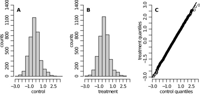
Human SILAC dataset—protein abundance score distributions obtained with SCAMPI (ILSE parameter estimates) are shown for control (A) and treatment (B). The quantile-quantile plot in C compares the two distributions. The line is passing through the origin and has a 45° angle (x = y). The abundance score distributions for control and treatment are directly comparable, as they are very similar (e.g. comparable median and quartiles).

Fig. 6.

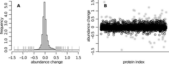
Human SILAC dataset—distribution of the difference between the protein abundance estimates in the treated and in the control case (D_j = Ĉ_j^treated − Ĉ_j^control). A, distribution of the estimated abundance changes. B, scatter plot of the protein identification number versus the estimated abundance difference. The two panels show essentially the same information. Particularly high score differences are highlighted (gray ticks in A and gray asterisks in B).

Note that one would typically require several biological replicates of each condition to test for significantly differentially abundant proteins. The scheme used above is a simplistic approach to illustrate what kinds of problems can be tackled using SCAMPI. If one has several biological replicates, SCAMPI can be run on each of them. More general testing approaches (e.g. a standard two-sample test or versions such as the moderated t test (e.g. 48)) should then be used to assess differential expression.

A direct comparison of SCAMPI's outcome with the results from MaxQuant (10) (normalized heavy-to-light ratios) is not straightforward. MaxQuant groups proteins and gives abundance scores to these groups. It is not clear how such a group abundance should be compared with the abundance scores for single proteins obtained in SCAMPI. However, there was some overlap between the outcomes of SCAMPI and MaxQuant: 15 of the 59 differentially expressed proteins (according to SCAMPI) also figured in one of the top-scoring groups identified by MaxQuant (see “SCAMPI Results Compared with MaxQuant Output” in the supplemental material).

Another aspect of SCAMPI, namely, the possibility of reassessing peptide abundance scores, was also demonstrated with the control condition of this last dataset. Based on the estimated parameter values and the graph structure, SCAMPI can be used to estimate peptide abundance scores (Û_i). These values can then be compared with the input data (U_i). The diagnostic plots (e.g. 49, 50) are shown in Fig. 7. Panels A (residual plot) and B (normal quantile-quantile plot) show no major violation of the assumptions regarding the noise term ϵ for the bulk of the data and can be used to select outliers (see “Selecting Outliers in the Measured Peptides” in the supplemental material for details). The 234 selected outliers are highlighted in panel B. This assessment allows us to gain further insight into the data on the peptide level by allowing us to check which peptides tend to have particularly large negative or positive residuals. In the present data, it can be observed that a large percentage of the peptides with a large negative residual (overestimated abundance) contained at least one missed cleavage. The assessment can also be used to prune the graph and rerun SCAMPI on this modified dataset to try to improve the protein abundance estimates. The output of such an iterative approach is provided in the supplemental material.

Fig. 7.

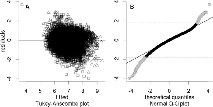
Human SILAC dataset—peptide abundance score reassessment for the control case in the SILAC-labeled human shotgun proteomics data. Triangles indicate information from shared peptides, and squares that from unique sequences. The residual plot in A (estimated scores (Û_i) versus residuals (R_i = U_i − Û_i)) does not show any major violations of the modeling assumptions. The normal quantile-quantile plot in B shows that the normality assumption on the errors is correct for the bulk of the data. Points marked by gray asterisks show the peptides that were selected as outliers.

Finally, a major aim of SCAMPI is to accurately model highly abundant shared peptides. Fig. 8 shows that this aim was achieved: SCAMPI was indeed able to explain highly abundant shared peptides extremely well and thus affirm that these measurements were correct and should not have been discarded as outliers.

Fig. 8.

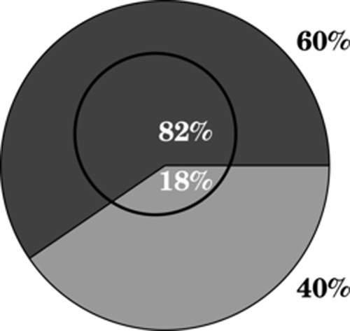
Human SILAC dataset—SCAMPI accurately modeled highly abundant shared peptides. In this example from the SILAC-labeled human shotgun proteomics data, the larger circle represents the 304 (1% of all peptides) sequences with the greatest input abundance scores for the control condition. 60% of these peptides were unique, and 40% were shared. The smaller circle represents the subpopulation of these peptides that also belonged to the 1% of peptides with the highest residuals. Among this subpopulation (73 sequences), 82% were unique peptides, and only 18% were shared. This shows that SCAMPI can explain highly abundant shared peptides extremely well and thus affirm that these measurements are correct and should not be regarded as outliers.

DISCUSSION

SCAMPI is a rigorous statistical approach for protein quantification on the basis of LC-MS/MS-based experiments. Our model explicitly accounts for dependences among and between peptides and proteins using a Markovian-type assumption for graphs. In contrast to most other protein quantification approaches, SCAMPI's modeling framework offers the following:

1. propagation of the uncertainty from the peptide identification to the protein level, leading to prediction intervals for proteins,

2. ability to reassess the peptide measurements based on the predicted protein concentration scores,

3. ability to handle different types of peptide abundance input scores, and

4. making use of all peptides in the input data, including the shared peptides.

Model Assumptions

Regarding the assumption of independent and identically distributed error terms, the residual plots for the analyzed datasets did not show any major violations. The other model assumptions cannot easily be checked. However, Markovian-type assumptions for graphs are often used in similar problems and allow one to account for at least some dependence (among and between peptides and proteins) while rendering the problem computationally tractable. Regarding the normality assumption for the protein abundances, if this is not fulfilled, the result provided by Equation 3 is still the best linear approximation for the estimate of Ĉ_j.

Using Log-transformed Input Data

For all examples presented here, the input peptide intensities were (base-10) log transformed. Applying a log transformation makes the data more symmetric and Gaussian. When working with peptide abundance scores, it typically makes sense to apply a log transformation before using them to infer protein abundances. After the transformation, the features are spread more evenly across the intensity range and the variability becomes constant at all intensity levels.

Uncertainty of Computed Scores

An important advantage of a model-based approach such as SCAMPI is the possibility of estimating the accuracy of the predicted scores. SCAMPI readily provides the variance of the abundance scores, which allows a prediction interval to be computed for each protein.

Parameter Estimation

The four model parameters (α, β, μ, and τ) are estimated based on the whole dataset. Thus, even though protein scores (and their variances) are computed “locally” on the corresponding connected component, knowledge gained about the whole dataset contributes to these parameter estimates. In particular, study of a protein matching a single quantified peptide will still benefit from the total knowledge about the dataset thanks to the global model parameters.

MLE versus ILSE Parameter Estimates

The results show that the parameter estimates obtained with the MLE and the ILSE approach (see “Parameter Estimation”) are often similar. Generally, when one compares the estimated protein scores with the ILSE and MLE estimated parameter sets, the differences become almost imperceptible. However, the computational bottleneck that occurs when analyzing a dataset is not a result of the choice of the parameter estimation method. The computationally expensive part is the preprocessing of the connected components, peptide and protein data frames, which is necessary for both parameter estimation approaches. Nevertheless, the ILSE approach seems to be more robust. MLE uses the R function dmvnorm, which works with the inverse of the covariance matrices. Depending on the choice of starting parameters, the optimization procedure can reach a state in which some of the connected components' covariance matrices become singular. A workaround is to restart the optimization procedure several times with different (random) starting values until success is achieved. This proved to be a feasible solution for all datasets presented in this manuscript; however, it can increase the computation time substantially.

Performance Comparison to the TOP3 Approach

When comparing a TOP3 approach to SCAMPI, one should keep in mind that the two models actually operate on different input data. The question arises as to what would happen if SCAMPI were run on the exact same input data as TOP3. This issue is discussed in the supplemental material (“SCAMPI on TOP3 Input”). Briefly, if one is willing to discard all data except those required for a strict TOP3, and if no model is required in order for one to be able to reassess peptide scores, then running TOP3 is the easier and faster way to get protein abundance estimates. If not, SCAMPI is the better approach, because it makes use of all information in the dataset (including the shared peptides).

Absolute Quantification

For datasets with anchor proteins (e.g. “SRM Experiment on Leptospira interrogans” (36) and “Directed MS Human Data” (42)), the linear fit between the computed abundance scores and the experimentally determined concentrations for these sequences can be used to predict the absolute concentrations of other proteins in the sample. The provided prediction intervals can be adapted accordingly.

Relative Quantification

Samples under different conditions (e.g. control and treatment) can also be compared with SCAMPI. As a general procedure, we suggest running SCAMPI on each replicate/condition separately. Typically, several (biological) replicates of each condition are required in order to test for differentially abundant proteins.

Running SCAMPI Iteratively

SCAMPI allows us to identify outliers in the input peptide abundance scores. Removing these outliers from the dataset and rerunning SCAMPI can lead to improved protein abundance estimates. An automatic iterative outlier removal, as is available in the protiq R package, is suitable for a first analysis. It is, however, important to go back to the list of rejected peptides and try to understand why outliers occurred. This can lead to further insight about the dataset, for example, by hinting at incomplete databases or by indicating potentially modified peptides that can be further investigated in order to possibly gain new biological information.

General Conclusion

In summary, SCAMPI is well suited to address the protein quantification problem on the basis of various types of LC-MS/MS-based experiments to compute absolute abundances, as well as for relative quantification. In contrast to many other approaches, it provides an estimate of the abundance for each single protein having some experimental peptide evidence. Proteins are neither discarded nor grouped, but the user could perform such selection/grouping operations prior to running SCAMPI. Prediction intervals for the scores allow one to get an idea about the confidence of the computed abundances. Finally, a method that allows for a feedback loop to reassess the quantification on the peptide level has the potential to provide new insight in LC-MS/MS datasets.

SCAMPI is implemented in the R package protiq (41), which is available on the Comprehensive R Archive Network (CRAN). It can be used to predict protein abundances and detect true outliers in peptide measurements and can potentially be used for designing future experiments.

Implementation

The model has been implemented in R (40), and the results were computed on the following system:

• R version 2.15.3 (2013-03-01), x86_64-unknown-linux-gnu

• Base packages: base, datasets, graphics, grDevices, methods, stats, utils

• Other packages: fortunes 1.5-0, plotrix 3.4-6, protiq 1.1, sfsmisc 1.0-23

• Loaded via a namespace (and not attached): BiocGenerics 0.2.0, graph 1.34.0, mvtnorm 0.9-9994, RBGL 1.32.1, tools 2.15.3

The implemented functions are available in the protiq package on the CRAN.

REFERENCES

- 1. Gerber S. A., Rush J., Stemman O., Kirschner M. W., Gygi S. P. (2003) Absolute quantification of proteins and phosphoproteins from cell lysates by tandem MS. Proc. Natl. Acad. Sci. U.S.A. 100, 6940–6945 [DOI] [PMC free article] [PubMed] [Google Scholar]
- 2. Silva J. C., Gorenstein M. V., Li G. Z., Vissers J. P. C., Geromanos S. J. (2006) Absolute quantification of proteins by LCMSE: a virtue of parallel MS acquisition. Mol. Cell. Proteomics 5, 144–156 [DOI] [PubMed] [Google Scholar]
- 3. Aebersold R., Mann M. (2003) Mass spectrometry-based proteomics. Nature 422, 198–207 [DOI] [PubMed] [Google Scholar]
- 4. Wang F. (2008) Biomarker Methods in Drug Discovery and Development. Humana Press, Totowa, NJ [Google Scholar]
- 5. Wysocki V. H., Resing K. A., Zhang Q., Cheng G. (2005) Mass spectrometry of peptides and proteins. Methods 35, 211–222 [DOI] [PubMed] [Google Scholar]
- 6. Käll L., Vitek O. (2011) Computational mass spectrometry-based proteomics. PLoS Comput. Biol. 7(12), e1002277. [DOI] [PMC free article] [PubMed] [Google Scholar]
- 7. Keller A., Nesvizhskii A. I., Kolker E., Aebersold R. (2002) Empirical statistical model to estimate the accuracy of peptide identifications made by MS/MS and database search. Anal. Chem. 74, 5383–5392 [DOI] [PubMed] [Google Scholar]
- 8. Käll L., Canterbury J. D., Weston J., Noble W. S., MacCoss M. J. (2007) Semi-supervised learning for peptide identification from shotgun proteomics datasets. Nat. Methods 4, 923–925 [DOI] [PubMed] [Google Scholar]
- 9. Tabb D. L., Fernando C. G., Chambers M. C. (2007) MyriMatch: highly accurate tandem mass spectral peptide identification by multivariate hypergeometric analysis. J. Proteome Res. 6, 654–661 [DOI] [PMC free article] [PubMed] [Google Scholar]
- 10. Cox J., Mann M. (2008) MaxQuant enables high peptide identification rates, individualized p.p.b.-range mass accuracies and proteome-wide protein quantification. Nat. Biotechnol. 26, 1367–1372 [DOI] [PubMed] [Google Scholar]
- 11. Martens L. (2011) Gel-Free Proteomics: Methods and Protocols, Vol. 753, pp. 359–371, Humana Press, New York, NY [Google Scholar]
- 12. Nesvizhskii A. I., Aebersold R. (2005) Interpretation of shotgun proteomic data. Mol. Cell. Proteomics 4, 1419–1440 [DOI] [PubMed] [Google Scholar]
- 13. Nesvizhskii A. I., Keller A., Kolker E., Aebersold R. (2003) A statistical model for identifying proteins by tandem mass spectrometry. Anal. Chem. 75, 4646–4658 [DOI] [PubMed] [Google Scholar]
- 14. Li Y. F., Arnold R., Li Y., Radivojac P., Sheng Q., Tang H. (2009) A Bayesian approach to protein inference problem in shotgun proteomics. J. Comput. Biol. 16, 1183–1193 [DOI] [PMC free article] [PubMed] [Google Scholar]
- 15. Ma Z. Q., Dasari S., Chambers M. C., Litton M. D., Sobecki S. M., Zimmerman L. J., Halvey P. J., Schilling B., Drake P. M., Gibson B. W., Tabb D. L. (2009) IDPicker 2.0: improved protein assembly with high discrimination peptide identification filtering. J. Proteome Res. 8, 3872–3881 [DOI] [PMC free article] [PubMed] [Google Scholar]
- 16. Gerster S., Qeli E., Ahrens C. H., Bühlmann P. (2010) Protein and gene model inference based on statistical modeling in k-partite graphs. Proc. Natl. Acad. Sci. U.S.A. 107, 12101–12106 [DOI] [PMC free article] [PubMed] [Google Scholar]
- 17. Serang O., MacCoss M. J., Noble W. S. (2010) Efficient marginalization to compute protein posterior probabilities from shotgun mass spectrometry data. J. Proteome Res. 9, 5346–5357 [DOI] [PMC free article] [PubMed] [Google Scholar]
- 18. Spivak M., Weston J., Tomazela D., MacCoss M. J., Noble W. S. (2012) Direct maximization of protein identifications from tandem mass spectra. Mol. Cell. Proteomics 11(2), M111.012161. [DOI] [PMC free article] [PubMed] [Google Scholar]
- 19. Carr S., Aebersold R., Baldwin M., Burlingame A., Clauser K., Nesvizhskii A. (2004) The need for guidelines in publication of peptide and protein identification data. Mol. Cell. Proteomics 3, 531–533 [DOI] [PubMed] [Google Scholar]
- 20. Mueller L. N., Rinner O., Schmidt A., Letarte S., Bodenmiller B., Brusniak M. Y., Vitek O., Aebersold R., Müller M. (2007) SuperHirn—a novel tool for high resolution LC-MS-based peptide/protein profiling. Proteomics 7, 3470–3480 [DOI] [PubMed] [Google Scholar]
- 21. Nonlinear Dynamics Ltd Progenesis LC-MS. http://www.nonlinear.com/products/progenesis/lc-ms/overview/
- 22. Bertsch A., Gröpl C., Reinert K., Kohlbacher O. (2011) OpenMS and TOPP: open source software for LC-MS data analysis. In Data Mining in Proteomics, Vol. 696, pp. 353–367, Humana Press, New York, NY: [DOI] [PubMed] [Google Scholar]
- 23. Ishihama Y., Oda Y., Tabata T., Sato T., Nagasu T., Rappsilber J., Mann M. (2005) Exponentially modified protein abundance index (empai) for estimation of absolute protein amount in proteomics by the number of sequenced peptides per protein. Mol. Cell. Proteomics 4, 1265–1272 [DOI] [PubMed] [Google Scholar]
- 24. Braisted J., Kuntumalla S., Vogel C., Marcotte E., Rodrigues A., Wang R., Huang S. T., Ferlanti E., Saeed A., Fleischmann R., Peterson S., Pieper R. (2008) The APEX quantitative proteomics tool: generating protein quantitation estimates from LC-MS/MS proteomics results. BMC Bioinformatics 9, 529. [DOI] [PMC free article] [PubMed] [Google Scholar]
- 25. Sun A., Zhang J., Wang C., Yang D., Wei H., Zhu Y., Jiang Y., He F. (2009) Modified spectral count index (mSCI) for estimation of protein abundance by protein relative identification possibility (RIPpro): a new proteomic technological parameter. J. Proteome Res. 8, 4934–4942 [DOI] [PubMed] [Google Scholar]
- 26. Clough T., Key M., Ott I., Ragg S., Schadow G., Vitek O. (2009) Protein quantification in label-free LC-MS experiments. J. Proteome Res. 8, 5275–5284 [DOI] [PubMed] [Google Scholar]
- 27. Griffin N. M., Yu J., Long F., Oh P., Shore S., Li Y., Koziol J. A., Schnitzer J. E. (2010) Label-free, normalized quantification of complex mass spectrometry data for proteomic analysis. Nat. Biotechnol. 28, 83–89 [DOI] [PMC free article] [PubMed] [Google Scholar]
- 28. Chang C. Y., Picotti P., Hüttenhain R., Heinzelmann-Schwarz V., Jovanovic M., Aebersold R., Vitek O. (2012) Protein significance analysis in selected reaction monitoring (SRM) measurements. Mol. Cell. Proteomics 11(4), M111.014662. [DOI] [PMC free article] [PubMed] [Google Scholar]
- 29. Domon B., Aebersold R. (2010) Options and considerations when selecting a quantitative proteomics strategy. Nat. Biotechnol. 28, 710–721 [DOI] [PubMed] [Google Scholar]
- 30. Jin S., Daly D. S., Springer D. L., Miller J. H. (2008) The effects of shared peptides on protein quantitation in label-free proteomics by LC/MS/MS. J. Proteome Res. 7, 164–169 [DOI] [PubMed] [Google Scholar]
- 31. Zhang Y., Wen Z., Washburn M. P., Florens L. (2010) Refinements to label free proteome quantitation: how to deal with peptides shared by multiple proteins. Anal. Chem. 82, 2272–2281 [DOI] [PubMed] [Google Scholar]
- 32. Dost B., Bandeira N., Li X., Shen Z., Briggs S. P., Vineet B. (2012) Accurate mass spectrometry based protein quantification via shared peptides. J. Comput. Biol. 19, 337–348 [DOI] [PMC free article] [PubMed] [Google Scholar]
- 33. Huang T., Gong H., Yang C., He Z. (2013) Proteinlasso: a lasso regression approach to protein inference problem in shotgun proteomics. Comput. Biol. Chem. 43, 46–54 [DOI] [PubMed] [Google Scholar]
- 34. Malmström J., Beck M., Schmidt A., Lange V., Deutsch E. W., Aebersold R. (2009) Proteome-wide cellular protein concentrations of the human pathogen Leptospira interrogans. Nature 460, 762–765 [DOI] [PMC free article] [PubMed] [Google Scholar]
- 35. Maier T., Schmidt A., Guell M., Kuhner S., Gavin A. C., Aebersold R., Serrano L. (2011) Quantification of mRNA and protein and integration with protein turnover in a bacterium. Mol. Syst. Biol. 7, 511. [DOI] [PMC free article] [PubMed] [Google Scholar]
- 36. Ludwig C., Claassen M., Schmidt A., Aebersold R. (2012) Estimation of absolute protein quantities of unlabeled samples by selected reaction monitoring mass spectrometry. Mol. Cell. Proteomics 11(3), M111.013987. [DOI] [PMC free article] [PubMed] [Google Scholar]
- 37. Lauritzen S. L. (1996) Graphical Models, Oxford Science Publications, New York, NY [Google Scholar]
- 38. Anderson T. W. (2003) An Introduction to Multivariate Statistical Analysis, John Wiley & Sons, Hoboken, NJ [Google Scholar]
- 39. Bickel P. J., Doksum K. A. (2001) Mathematical Statistics; Basic Ideas and Selected Topics, Vol. 1, 2nd Ed., Prentice-Hall, New Jersey [Google Scholar]
- 40. R Development Core Team (2011) R: A Language and Environment for Statistical Computing. R Foundation for Statistical Computing, Vienna, Austria [Google Scholar]
- 41. Gerster S., Bühlmann P. (2012) protiq: protein (identification and) quantification based on peptide evidence. R package version 1.1. R Foundation for Statistical Computing, Vienna, Austria [Google Scholar]
- 42. Beck M., Schmidt A., Malmstroem J., Claassen M., Ori A., Szymborska A., Herzog F., Rinner O., Ellenberg J., Aebersold R. (2011) The quantitative proteome of a human cell line. Mol. Syst. Biol. 7, 549. [DOI] [PMC free article] [PubMed] [Google Scholar]
- 43. Altman D. G., Bland J. M. (1983) Measurement in medicine: the analysis of method comparison studies. J. R. Stat. Soc. Series D Statistician 32, 307–317 [Google Scholar]
- 44. Mitsiades N., Mitsiades C. S., Poulaki V., Chauhan D., Fanourakis G., Gu X., Bailey C., Joseph M., Libermann T. A., Treon S. P., Munshi N. C., Richardson P. G., Hideshima T., Anderson K. C. (2002) Molecular sequelae of proteasome inhibition in human multiple myeloma cells. Proc. Natl. Acad. Sci. U.S.A. 99, 14374–14379 [DOI] [PMC free article] [PubMed] [Google Scholar]
- 45. Bieler S., Meiners S., Stangl V., Pohl T., Stangl K. (2009) Comprehensive proteomic and transcriptomic analysis reveals early induction of a protective anti-oxidative stress response by low-dose proteasome inhibition. Proteomics 9, 3257–3267 [DOI] [PubMed] [Google Scholar]
- 46. Zhang L., Chang M., Li H., Hou S., Zhang Y., Hu Y., Han W., Hu L. (2007) Proteomic changes of pc12 cells treated with proteasomal inhibitor psi. Brain Res. 1153, 196–203 [DOI] [PubMed] [Google Scholar]
- 47. Weinkauf M., Zimmermann Y., Hartmann E., Rosenwald A., Rieken M., Pastore A., Hutter G., Hiddemann W., Dreyling M. (2009) 2-d page-based comparison of proteasome inhibitor bortezomib in sensitive and resistant mantle cell lymphoma. Electrophoresis 30, 974–986 [DOI] [PubMed] [Google Scholar]
- 48. Smyth G. K. (2004) Linear models and empirical bayes methods for assessing differential expression in microarray experiments. Stat. Appl. Genet. Mol. Biol. 3(1), Article 3 [DOI] [PubMed] [Google Scholar]
- 49. Rawlings J. O., Pantula S. G., Dickey D. A. (1998) Applied Regression Analysis—A Research Tool, 2nd Ed., Springer, New York, NY [Google Scholar]
- 50. Sheather S. J. (2009) A Modern Approach to Regression with R, Springer, New York, NY [Google Scholar]
Associated Data
This section collects any data citations, data availability statements, or supplementary materials included in this article.