

Abstract
Structure learning of Bayesian Networks (BNs) is an important topic in machine learning. Driven by modern applications in genetics and brain sciences, accurate and efficient learning of large-scale BN structures from high-dimensional data becomes a challenging problem. To tackle this challenge, we propose a Sparse Bayesian Network (SBN) structure learning algorithm that employs a novel formulation involving one L1-norm penalty term to impose sparsity and another penalty term to ensure that the learned BN is a Directed Acyclic Graph (DAG)—a required property of BNs. Through both theoretical analysis and extensive experiments on 11 moderate and large benchmark networks with various sample sizes, we show that SBN leads to improved learning accuracy, scalability, and efficiency as compared with 10 existing popular BN learning algorithms. We apply SBN to a real-world application of brain connectivity modeling for Alzheimer’s disease (AD) and reveal findings that could lead to advancements in AD research.
Keywords: Bayesian network, machine learning, data mining
1 INTRODUCTION
A Bayesian network (BN) is a graphical model for representing the probabilistic relationships among variables. BNs have been widely used in the fields of genetics [1], [2], ecology [3], [4], social sciences [5], medical sciences [6], brain sciences [7], [8], and manufacturing [9]. A BN consists of two components: the structure, which is a Directed Acyclic Graph (DAG), for representing the dependency and independency among variables, and a set of parameters for representing the quantitative information of the dependency. Accordingly, learning a BN from data includes structure learning and parameter learning. This paper focuses on structure learning.
One type of structure learning method is constraint based. Constraint-based methods [10], [11], [12], [13], [14] use conditional independence tests to identify the dependent and independent relationships among variables. A major weakness of these methods is that too many tests may have to be performed, with each test being built upon the results of another, leading to escalated errors in the BN structure identification.
Another type of structure learning method is score based, in which a “score” is defined for each possible BN structure and then a search algorithm is used to find the structure with the highest score. Various score functions have been proposed, including those based on the Bayesian method [15], [16], [17], [18], [19], minimum description length [20], [21], [22], [23], and entropy [10], [24]. Furthermore, once a score function is specified, a search method is needed to find the structure with the highest score. Because the number of possible structures grows exponentially with respect to the number of variables, an exhaustive search over all possible structures may be computationally too expensive or unfeasible. Therefore, various inexact search methods have been proposed, such as heuristic search techniques [15], [24], [25], [26], genetic algorithms [28], [29], and simulated annealing [30]. Sampling methods such as Markov Chain Monte Carlo (MCMC) [18], [24] have also been utilized to travel through the DAG space. These methods usually find a BN structure that is a local optimum, and have been less effective in high-dimensional DAG spaces. In addition, some work has been done to combine score-based methods with constraint-based methods [31]. Then there is the recently developed novel additive noise model [32], which differs from both constraint-based and score-based methods and has the advantage of learning nonlinear interactions for non-Gaussian BNs.1
Driven by modern applications in brain sciences and genetics, there has been a great need of algorithms capable of learning large BN structures with high accuracy and efficiency from limited samples. For example, BNs provide an effective tool for identifying how different brain regions interact with each other in task performance, skill learning, and disease processes from neuroimaging data [7], [8]. A typical neuroimaging dataset includes hundreds of variables (brain regions), while the sample size (number of experimental subjects) is usually in tens. Also, BNs are very useful for modeling the interacting patterns between genes from microarray gene expression data, which measures thousands of genes with sample size being no more than a few hundred [1], [2].
For the purpose of learning a large BN with small sample sizes, a useful strategy is to impose a “sparsity” constraint of some kind. Many real-world networks are indeed sparse, such as the gene association networks [1], [33] and brain connectivity networks [34]. When learning the structure of these networks, a sparsity constraint helps prevent over-fitting and improves computational efficiency. For example, the Sparse Candidate (SC) algorithm [35], one of the first large-scale BN structure learning algorithms, achieves sparsity by assuming that the maximum number of parents for each node is limited to a small constant. One major problem with SC is that the user has to guess the maximum number of parents. Also, it is usually unrealistic to assume that all the nodes have the same maximum number of parents. The L1MB-DAG algorithm [36] does not require a prior specification on the maximum number of parents. Instead, it uses LASSO to select a small set of potential parents for each variable. LASSO is known for sparse variable selection [37].
In addition to the sparsity consideration, recently developed BN structure learning methods usually consist of two stages: Stage 1 is to identify the potential parents of each variable; Stage 2 applies some search methods to identify the parents out of the potential parent set. The advantage of the two-stage approach is improved efficiency, as Stage 2 is a local search over a possibly small set of potential parents for each variable identified by Stage 1, rather than a global search over all the variables. The two-stage approach has been popularly adopted by many existing algorithms, including the SC and the L1MB-DAG algorithms, mentioned previously, as well as the Hill-Climbing (MMHC) [38], the Grow-Shrink [39], the TC, and the TC-bw [40] algorithms. The difference between these algorithms primarily lies in how they identify the potential parent set in Stage 1. For example, L1MB-DAG uses LASSO, MMHC uses the G2 statistic, and TC and TC-bw use a t-test. An apparent weakness of the two-stage approach is that if a true parent is missed in Stage 1, it will never be recovered in Stage 2. Another weakness of the existing algorithms is that the computational efficiency is still too low for learning large BNs. For example, it may take hours or days to learn a BN with 500 nodes.
In this paper, we propose a new sparse Gaussian BN structure learning algorithm called Sparse Bayesian Network (SBN). It is a one-stage approach that identifies the parents of all variables directly, thus having a low risk of missing parents (i.e., a high accuracy in BN structure identification) compared with many existing algorithms that employ the two-stage approach. Specifically, in development of the SBN, we propose a novel formulation with one L1-norm penalty term to impose sparsity and another penalty term to ensure that the learned BN is a Directed Acyclic Graph—a required property of BN. The theoretical property about how to select the regularization parameter associated with the second penalty term is discussed. Under this formulation, we propose to use the Block Coordinate Descent (BCD) and shooting algorithms to estimate the BN structure. Further, our theoretical analysis indicates that the computational complexity of SBN is linear in the sample size and quadratic in the number of variables. This characteristic makes SBN more scalable and efficient than most existing algorithms, and thus well suited for large-scale BN structure learning from high-dimensional datasets.
In addition, we perform theoretical analysis to show why the two-stage approach popularly adopted in the existing literature has a high risk of misidentifying the true parents and how the proposed SBN overcomes this deficiency. Also, extensive experiments on synthetic data are performed to compare SBN and the existing algorithms in terms of the learning accuracy, scalability, and efficiency. Finally, we apply SBN to a real-world application of brain connectivity modeling for Alzheimer’s disease (AD). In particular, SBN is applied to the neuroimaging PDG-PET data of 42 AD patients and 67 matching normal control (NC) subjects in order to identify the brain connectivity model for each of the two study groups. A connectivity model represented by a BN reveals the directional effects of one brain region over another—called the effective connectivity. Effective connectivity has been much less studied in the AD literature, as most existing work focuses on functional connectivity, i.e., the correlations among brain regions. In this sense, the application of SBN to AD has the advantage over undirected graphical models of providing new insights into the mechanisms/pathways that distinct brain regions communicate with each other. In this application, the effective connectivity model of AD identified by SBN is compared in many different ways with that of NC, including the connectivity at the global scale, intra/interlobe and inter-hemisphere connectivity distribution, and the connectivity associated with specific brain regions. The findings are consistent with known pathology and the clinical progression in AD.
The rest of the paper is organized as follows: Section 2 introduces the key definitions and concepts of BN. Section 3 presents the development of SBN. Section 4 performs a theoretical analysis on the competitive advantage of SBN over the existing algorithms that employ the two-stage approach. Section 5 presents the results of the experiments on synthetic data. Section 6 presents the application of SBN to brain connectivity modeling of AD. Section 7 is the conclusion.
2 Bayesian Network: Key Definitions and Concepts
In this section, we give a brief introduction to the key definitions and concepts of BNs:
A BN is composed by a structure and a set of parameters. The structure (Fig. 1) is a DAG that consists of p nodes [X1,…, Xp] and directed arcs between some nodes; no cycle is allowed in a DAG. Each node represents a random variable. In this paper, we will use nodes and variables interchangeably. The directed arcs encode the dependent and independent relationships among the variables. If there is a directed arc from Xi to Xj, Xi is called a parent of Xj and Xj is called a child of Xi. Two nodes are called spouses of each other if they share a common child. If there is a directed path from Xi to Xj, i.e., Xi → ⋯ → Xj, Xi is called an ancestor of Xj. A directed arc is also a directed path and a parent is also an ancestor according to this definition. The Markov Blanket (MB) of Xj is a set of variables and, given this set of variables, Xj will be independent of all other variables. The MB consists of the parents, children, and spouses of Xj.
Fig. 1.
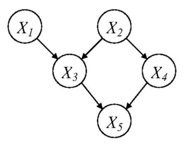
A Bayesian network structure (DAG).
In this paper, we will adopt the following notations with respect to a BN structure: We denote the structure by a p × p matrix G, with entry Gij = 1 representing a directed arc from Xi to Xj and Gij = 0, otherwise. The set of parents of a node Xi is denoted by PA(Xi). In addition, we define a p × p matrix, P, which records all the directed paths in the structure, i.e., if there is a directed path from Xi to Xj, entry Pij = 1; otherwise, Pij = 0.
In addition to the structure, another important component of a BN is the parameters. The parameters are the conditional probability distribution of each node given its parents. Specifically, when the nodes follow a multivariate normal distribution, a regression-type parameterization can be adopted, i.e., with and βi being a vector of regression coefficients. Without loss of generality, we assume in this paper that the nodes are standardized, i.e., each with a zero mean and unit variance. Then, the parameters of a BN are B = [β1,…, βp].
3 The Proposed Sparse BN Structure Learning Algorithm—SBN
One of the challenging issues in BN structure learning is to ensure that the learned structure must be a DAG, i.e., no cycle is present. To achieve this, we first identify a sufficient and necessary condition for a DAG
Lemma 1
A sufficient and necessary condition for a DAG is βji × Pij = 0 for every pair of nodes Xi and Xj.
Proof
To prove the necessary condition, suppose that a BN structure, G, is a DAG. Let’s assume that βji × Pij ≠ 0 for a pair of nodes Xi and Xj. Then, there exists a directed path from Xj to Xi and a directed path from Xi to Xj, i.e., there is a cycle in G which is a contradiction to our presumption that G is a DAG. To prove the sufficient condition, suppose that βji × Pij = 0 for every pair of nodes Xi and Xj. If G is not a DAG, i.e., there is a cycle, it means that there exist two variables, Xi and Xj, with a directed arc from Xj to Xi (βji ≠ 0) and a directed path from Xi to Xj (Pij = 1). This is a contradiction to our presumption that βji × Pij = 0 for every pair of nodes Xi and Xj.
Based on Lemma 1, we further present our formulation for sparse BN structure learning. It is an optimization problem with the objective function and constraints given by
| (1) |
According to the definition of P, P is a function of B. So the constraints in (1) are functions of B. The notations in (1) are explained as follows: xi = [xi1,…, xin] denote the sample vector for Xi, where n is the sample size. x/i denotes the sample matrix for all the variables except Xi. The first term in the objective function, , is a profile likelihood to measure the model fit. In the second term, ∥βi∥1 is the sum of the absolute values of the elements in βi and thus is the so-called L1-norm penalty [37]. The regularization parameter, λ1, controls the number of nonzero elements in the solution to βi, ; the larger the λ1, the fewer nonzero elements in . Because fewer nonzero elements in correspond to fewer arcs in the learned BN structure, a larger λ1 results in a sparser structure. In addition, the constraints are to assure that the learned BN is a DAG (see Lemma 1 and Theorem 1 below).
Solving the constrained optimization in (1) is difficult. Therefore, the penalty method [42] is employed to transform it into an unconstrained optimization problem, through adding an extra L1-norm penalty into the objective function, i.e.,
| (2) |
where j⋐X/i denotes that the variable indexed by j, i.e.,Xj, is a variable different from Xi. Here, λ2 ∑j⋐X/i |βji× Pij| is to push βji × Pij to become zero. Under some mild conditions [42], there exists a such that for all , is also a minimizer for (1). Later, in Theorem 1, we will show how to derive a practical estimation for .
Given λ1 and λ2, the BCD algorithm [43] can be employed to solve (2). The BCD algorithm updates each βi iteratively, assuming that all other parameters are fixed. In our situation, this is equivalent to optimizing fi(βi) in (3) iteratively and the algorithm will terminate when some convergence conditions are satisfied. We remark that fi(βi), after some transformation, is similar to LASSO [37], i.e.,
| (3) |
As a result, the shooting algorithm [44] for LASSO may be used to optimize fi(βi) in each iteration. Note that at each iteration for optimizing fi(βi), we also need to calculate Pij for j⋐X/i. This can be done by a Breadth-first search on G with Xi being the root node [45]. A more detailed description of the BCD algorithm and the shooting algorithm used to solve (3) is given in Figs. 2 and 3, respectively.
Fig. 2.

The BCD algorithm used for solving (2).
Fig. 3.

The shooting algorithm used for solving (3).
Choosing two free parameters, λ1 and λ2, may be a difficult task in practice. Fortunately, Theorem 1 shows that, with a given λ1, any λ2 > (n – 1)2p/λ1 – λ1 will guarantee the output the BCD algorithm to be a DAG.
Theorem 1
Any λ2 > (n – 1)2p/λ1 – λ1 will guarantee to be a DAG.
Proof
To prove this, we first need to prove that, with a certain value of λ1 and any value of λ2, is bounded, i.e., , for each . The second inequality holds because is the value of the left-hand side of the inequality when βi = 0, which is obviously larger than that when . The last equality holds because we have standardized all the variables. Thus we know that . Now, we use proof-by-contradiction to show that, with any λ2 > (n – 1)2p/ λ1 – λ1, we will get a DAG. Suppose that such a λ2 doesn’t guarantee a DAG. Then, there must be at least a pair of variables Xi and Xj with βji × Pij ≠ 0, which is βji ≠ 0 and Pij = 1, based on the first order optimality condition, βji ≠ 0, i.f.f. . Here, denotes the elements in without and x/(i,j) denotes the sample matrix for all the variables except Xi and Xj. However,
resulting in .
Theorem 1 implies that if we specify any λ2 > (n – 1)2p/ λ1 – λ1, we will get a minimizer of (1) through solving (2). However, in practice, directly solving (2) by specifying a large λ2 may converge slowly. This is because the unconstrained problem in (2) may be ill-conditioned with a too large value for λ2 [42]. To avoid this situation, the “warm start” method [42] can be used, which works in the following way: First, it specifies a series of values for λ2, i.e., , with a small and ; next, it optimizes (2) with to get a minimizer , using an arbitrary initial value; then, it optimizes (2) with , using as an initial value; this process iterates until it optimizes (2) with . With the last minimizer as the initial value for the next optimization problem, this method can be quite efficient.
Finally, we want to mention that the L2-norm penalty, λ2 ∑j⋐X/i (βji × Pij)2, might also be used in (2). The advantage is that it is a differentiable function of βji. Also, as shown in [42], βji × Pij → 0 when λ2 → ∞. However, the weakness of the L2-norm penalty, compared with the L1-norm penalty, is that there is no guarantee that a finite λ2 exists to assure βji × Pij = 0 for all pairs of Xi and Xj.
Time complexity analysis
Each iteration of the BCD algorithm consists of two operations: a shooting algorithm and a Breadth-first search on G. These two operations cost O(pn) [46] and O(p + |G|), respectively. Here, |G| is the number of nonzero elements in G. If G is sparse, i.e., |G| = Cp with a small constant C, then O(p + |G|) = O(p). Thus, the computational cost at each iteration is only O(pn). Furthermore, each sweep through all columns of B costs O(p2n). Our simulation study shows that it usually takes no more than 5 sweeps to converge.
4 Some Theoretical Analysis on the Competitive Advantage of the Proposed SBN Algorithm
Simulation studies in Section 5 will show that SBN is more accurate than various existing algorithms that employ a two-stage approach. This section aims to provide some theoretical insights about why the existing algorithms are less accurate. Please note that although a comprehensive analysis of this kind on all types of BNs and all two-stage algorithms is the most desirable, it is also very challenging, if not impossible, and beyond the scope of this paper. Therefore, in this section, we focus on some specific types of BNs and one popular two-stage algorithm, so as to provide some supporting evidence for the proposed SBN in addition to the results of the simulation studies in Section 5.
Recall that Stage 1 of the two-stage approach is to identify the potential parents of each Xi. The existing algorithms achieve this goal by identifying the MB of Xi. A typical method is variable selection based on regressions, i.e., to build a regression of Xi on all other variables and consider the variables selected to be the MB. One difference between various algorithms is the type of regression used and the method used for variable selection. For example, the TC algorithm [40] uses ordinary regression and a t-test for variable selection; the L1MB-DAG algorithm [36] uses LASSO.
However, in the regression of Xi, not only will the coefficients for the variables not in the MB be small (theoretically zero due to the definition of MB), the coefficients for the parents may also be very small due to the correlation between the parents and the children. As a result, some parents may not be selected in the variable selection, i.e., they will be missed in Stage 1 of the two-stage approach, leading to greater BN learning errors. In contrast, SBN may not suffer from this problem because it is a one-stage approach that identifies the parents directly.
To further illustrate this point, we analyze one two-stage algorithm, the TC algorithm. TC does variable selection using a t-test. To determine whether a variable should be selected, a t-test uses the statistic , where is the least-square estimate for the regression coefficient of this variable and is the standard error. The larger the value of the higher the chance that the variable will be selected. Theorems 2 and 3 below show that even though the value of corresponding to a parent of Xi is large in the true BN, its value may decrease drastically in the regression of Xi on all other variables. Theorem 2 focuses on a specific type of BN, a general tree, in which all variables have one common ancestor and there is at most one directed path between two variables; Theorem 3 focuses on a general inverse tree, which becomes a general tree if reversing all the arcs. Proof of Theorem 2 can be found in Appendix A, which can be found on the Computer Society Digital Library at http://doi.ieeecomputersociety.org/10.1109/TPAMI.2012.130. Proof of Theorem 3 can also be found in the supplemental material available online.
Theorem 2
Consider a general tree with m variables, whose structure and parameters are given by X1 = e1, X2 = β12X1 + e2, Xi = β2iX2 + ei, i = 3,4, …, m (Fig. 4). All the variables have unit variance. Let denote the least-square estimate for β12 in regression X2 = β12X1 + e2. Let denote the least-square estimate for in regression (i.e., a regression that regresses X2 on all other variables in the general tree).Then, the following relations hold:
where denotes the least-square estimate for a regression coefficient βij and denotes the standard error for .
Fig. 4.
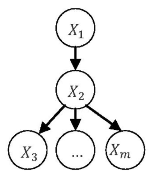
A general tree.
Theorem 3
Consider a general inverse tree with m + l + 2 variables, whose structure and parameters are given by
(Fig. 5). All the variables have unit variance. Let denote the least-square estimate for βk,l+1 in regression , k = 1,2,…,l. Let denote the least-square estimate for in regression (i.e., a regression that regresses Xl+1 on all other variables in the general inverse tree). Then, the following relations hold:
Fig. 5.
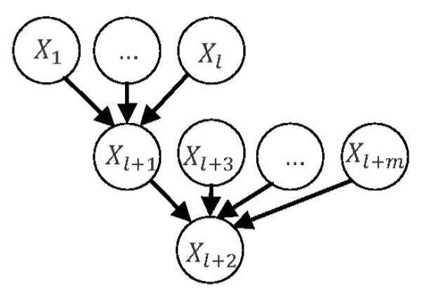
A general inverse tree.
Here, we use two examples to illustrate the theorems. Consider a general tree with m = 8 (see Fig. 4 to recall the definition for m) and least-square estimates for the parameters being and , i = 3, …, 8. Then, using the formula for in Theorem 2, we can get . Using the formula for , we can get . Consider a general inverse tree with l = 5 and m = 0 (see Fig. 5 to recall definitions for l and m) and least-square estimates for the parameters being and . Then, using the formula for (i.e., , k = 1, …, 5) in Theorem 3, we can get
Note that the theoretical study in this section focuses on Stage 1 of the two-stage approach. It would also be interesting to analyze Stage 2, e.g., to find out the relative significance of the coefficients for variables in the MB and identify under what conditions the true parents may be missed. We plan to conduct such analysis in the future.
5 Simulation Study on Synthetic Data
We perform five simulations. The first two show that, on a general tree and a general inverse tree, the existing algorithms based on the two-stage approach may miss some true parents with a high probability, while SBN performs well. The third simulation is to compare the structure learning accuracy of SBN with other competing algorithms using some benchmark networks. The fourth and fifth simulations are to investigate the scalability and efficiency of SBN and compare it with other competing algorithms. The code is available at http://www.public.asu.edu/~shuang31/codes/SBN.rar.
5.1 Learning Accuracy for General Tree
We select 10 existing algorithms in our study: HITON-PC [47], IAMB and three of its variants [48], GS [39], SC [35], TC and its advanced version TC-bw [40], and L1MB-DAG [36]. We focus on the general tree shown in Fig. 6a in which the regression coefficient of each arc is randomly generated from ±Uniform(0.5, 1). We simulate data from this general tree with a sample size of 200.
Fig. 6.

(a) General tree used in the simulation study in Section 5.1; (b) general inverse tree used in the simulation study in Section 5.2 (regression coefficients of arcs generated from ±Uniform(0.5, 1)).
We apply the selected existing algorithms on the simulated data; the parameters of each algorithm are selected in the way that has been suggested in the respective paper. Specifically, HITON-PC is applied with a significance level of 5 percent used in the G2 test of statistical independence and degrees of freedom set according to reference 14 cited in the paper of HITON-PC [47]. IAMB and its variants are applied with the significant level set to be 5 percent. GS is applied using the default value of 0.05 in its algorithm. SC is applied using the Bayesian scoring heuristic and the maximum number of parents chosen for the SC algorithm to be 5 and 10 (the one with better performance is kept and its corresponding result is presented). TC and TC-bw are applied by setting parameter α = 2/(p(p – 1)) as suggested and adopted in the paper [40]. There is no free parameter in L1MB-DAG.
In applying the proposed SBN, λ1 is selected by BIC (i.e., a step search is employed to find the λ1 that produces the minimum BIC value). Following Theorem 1, λ2 is set to be 10[(n – 1)2p/ λ1 – λ1], which empirically guarantees a DAG to be learned. Furthermore, note that the optimization problem in (2) is nonconvex, so a good initial value for B would be helpful. We tried various options and found that a good initial value can be the output from Stage 1 of the two-stage approaches (i.e., the potential parent set). Specifically, in our experiments we set the initial value to be the output from Stage 1 of L1MB, which is a parameter-free algorithm that can be easily assembled with SBN.
The results averaged over 100 repetitions are shown in Figs. 7a, 7b, and 7c. The X-axis records the 10 selected algorithms and the proposed SBN (the last one). The Y -axis of each figure in Figs. 7a, 7b, and 7c is a different performance measure, i.e., the frequency for X1 being identified as a parent of Xi, i = 2, …, 7, in (a), the ratio of the number of correctly identified arcs in the learned BN to the number of arcs in the true BN in (b), and the ratio of the total learning error in the learned BN (false positives plus false negatives) to the number or arcs in the true BN in (c). Note that Fig. 7a focuses on the arcs between X1 and Xi, i = 2, … 7, in order to demonstrate Theorem 2 (i.e., because the MB of Xi includes not only parent X1 but also six children, the coefficient of the arc between parent X1 and Xi may be underestimated so that X1 may not be included in the MB identified in Stage 1 of the competing algorithms). The observation from Fig. 7a is consistent with this theoretical explanation, which shows that the competing algorithms do not perform as well as SBN. Figs. 7b and 7c are performance measures defined on all arcs. They also show SBN’s better performance.
Fig. 7.
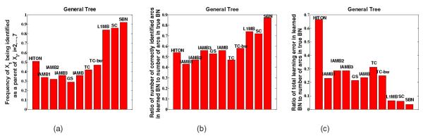
(a) Frequency of X1 being identified as a parent of Xi, i = 2, …, 7; (b) ratio of number of correctly identified arcs in learned BN to number of arcs in true BN; (c) ratio of total learning error in learned BN (false positives plus false negatives) to number of arcs in true BN.
5.2 Learning Accuracy for General Inverse Tree
We focus on the general inverse tree in Fig. 6b, in which the regression coefficient of each arc is randomly generated from ±Uniform(0.5, 1). We simulate data from this general with a sample size of 200.
We apply the 10 selected existing algorithms and SBN on the simulated data in the same way as that in Section 5.1. The results of 100 repetitions are shown in Figs. 8a, 8b, 8c, which can be read in a similar way to Fig. 7. Note that Fig. 8a focuses on the arcs between Xi, i = 1, …, 30, and their respective children in order to demonstrate Theorem 3. Figs. 8a, 8b, 8c show that SBN performs better.
Fig. 8.
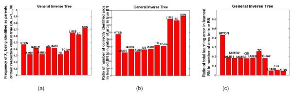
(a) Frequency of Xi being identified as parents of their respective child in true BN, i = 1, …, 30; (b) ratio of number of correctly identified arcs in learned BN to number of arcs in true BN; (c) ratio of total learning error in learned BN (false positives plus false negatives) to number of arcs in true BN
5.3 Learning Accuracy for Benchmark Networks
To evaluate the performance of SBN on general (i.e., non-tree-like) BNs, we select seven moderately large networks from the Bayesian Network Repository (BNR) [49]. None of these networks are tree-like except for the “Chain” network. These networks are selected based on the consideration that they provide a range of small-to-moderately-large networks with the number of nodes ranging from 7 to 61, they are sparse, and they were also used in [36], which is a competing algorithm of ours. We also use the tiling technique [50] to produce two large BNs, Alarm2, and Hailfinder2. Two other networks with specific structures, Factor and Chain [51], are also considered. The numbers of nodes and arcs in each of the 11 networks are shown in Table 1.
TABLE 1.
Benchmark Networks
| Networks | Number of nodes |
Number of arcs |
|
|---|---|---|---|
| 1 | Factor | 27 | 68 |
| 2 | Alarm (BNR) | 37 | 46 |
| 3 | Barley (BNR) | 48 | 84 |
| 4 | Carpo (BNR) | 61 | 74 |
| 5 | Chain | 7 | 6 |
| 6 | Hailfinder (BNR) | 56 | 66 |
| 7 | Insurance (BNR) | 27 | 52 |
| 8 | Mildew (BNR) | 35 | 46 |
| 9 | Water (BNR) | 32 | 66 |
| 10 | Alarm 2 | 296 | 410 |
| 11 | Haifinder 2 | 280 | 390 |
To specify the parameters of a network, i.e., to specify the regression coefficients of each variable on its parents, we randomly sample from ±Uniform(0.5, 1). Then, we data for each network with a sample size 1,000, and apply the 10 competing algorithms and SBN to learn the BN structure. The results over 100 repetitions are shown in Fig. 9a, in which the X-axis records the 11 networks and the Y -axis records the ratio of the total learning error in the learned BN (false positives plus false negatives) to the number of arcs in the true BN. This figure deserves more explanation: We found it hard to show all 10 competing algorithms, i.e., they become indistinguishable. Thus, for each benchmark network (i.e., a tick on the X-axis), we only show the three competing algorithms with the best performance. For example, for network “Carpo” (fourth tick on the X-axis) in Fig. 9a, the top three competing algorithms shown are GS, TC, and SC. Figs. 9b, 9c, 9d are comparison plots in terms of other criteria. Specifically, Fig. 9b plots the ratio of the correctly identified arcs in the learned BN (i.e., true positives) to the number of arcs in the true BN. Fig. 9c plots the ratio of the falsely identified arcs in the learned BN (i.e., false positives) to the number of arcs in the true BN. Fig. 9d is similar to Fig. 9a but for Partially Directed Acyclic Graph (PDAG). Given a BN (a learned one or true one), the corresponding PDAG can be obtained by the method proposed in [13]. A PDAG is a collection of statistically equivalent BN structures, i.e., these structures all represent the same set of dependent and independent relationships so they are statistically indistinguishable. The PDAG of a BN can be constructed by replacing a directed arc between Xi and Xj in the BN with an undirected one, if some statistically equivalent BN structures have Xi → Xj and others have Xi ← Xj. A PDAG is very useful when making a causal interpretation, i.e., we may interpret the directed arcs in the PDAG as representing the direction of direct causal influence. Figs. 9a, 9b, 9c, 9d show that SBN performs much better than all the competing algorithms in BN- and PDAG-identification.
Fig. 9.

(a) Ratio of total learning error in the learned BN (false positives plus false negatives) to the number of arcs in the true BN for the 10 competing algorithms and SBN on 11 benchmark networks; (b) ratio of correctly identified arcs in the learned BN (i.e., true positives) to the number of arcs in the true BN; (c) ratio of falsely identified arcs in the learned BN (i.e., false positives) to the number of arcs in the true BN; (d) ratio of the total learning error in the learned PDAG to the number of arcs in the true PDAG. The learned BN and PDAG in (a)-(d) are based on a simulation dataset of sample size 1,000. Dots are means and error bars are standard deviations.
Furthermore, we would like to compare SBN with the competing algorithms under small sample sizes. We decrease the sample size to 100 and repeat the above procedure. The results are shown in Figs. 10a, 10b, 10c, 10d. It can be seen that SBN still performs much better than all the competing algorithms in BN- and PDAG-identification even for small sample sizes.
Fig. 10.

(a) Ratio of total learning error in the learned BN (false positives plus false negatives) to the number of arcs in the true BN for the 10 competing algorithms and SBN on 11 benchmark networks; (b) ratio of correctly identified arcs in the learned BN (i.e., true positives) to the number of arcs in the true BN; (c) ratio of falsely identified arcs in the learned BN (i.e., false positives) to the number of arcs in the true BN; (d) ratio of the total learning error in the learned PDAG to the number of arcs in the true PDAG. The learned BN and PDAG in (a)-(d) are based on a simulation dataset of sample size 100. Dots are means and error bars are standard deviations.
5.4 Scalability
We study two aspects of scalability for SBN: the scalability with respect to the number of variables in a BN, p, and the scalability with respect to the sample size, n. We use the CPU time for each sweep through all the columns of B as the parameter for measurement. Specifically, we fix n = 1,000, and vary p by using the 11 benchmark networks. Also, we fix p = 37 (the Alarm network). The results over 100 repetitions are shown in Figs. 11a and 11b, respectively. It can be seen that the times are linear in n and quadratic in p, which confirms our theoretical time complexity analysis in Section 3.
Fig. 11.
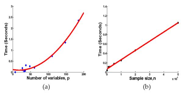
Scalability of SBN with respect to (a) the number of variables, p, (b) the sample size, n.
5.5 Efficiency
We further compare the CPU time of SBN with other competing algorithms in structure learning of the 11 benchmark networks. In particular, the CPU time of SBN is the time it takes the algorithm in Fig. 2 to converge for given regularization parameters and initial value. The CPU times of other competing algorithms are recorded in a similar way. The results of 100 repetitions are shown in Table 2 (the two large networks, Alarm 2 and Haifinder 2) and Fig. 12 (the other networks). It can be seen that SBN is the fastest algorithm in structure learning of all the benchmark networks. This is expected since the fastest algorithms among the 10 competing algorithms, i.e., GS and TC, have a time complexity O(p3n), while SBN only costs O(p2n) (i.e., each sweep of SBN costs O(p2n) and our simulation study shows that SBN usually takes no more than five sweeps to converge).
TABLE 2.
Comparison of SBN with Competing Algorithms on the CPU Time in Structure Learning of Two Large Networks (Standard Derivation Is Shown in the Bracket)
| Algorithms | Alarm 2 | Haifinder 2 |
|---|---|---|
| SBN | 67.1 (13.4) | 78.8 (19.5) |
| SC | 958 (73.6) | 987 (83.2) |
| L1MB-DAG | 11715 (1034.8) | 13521 (2543.3) |
| GS | 1071 (142.4) | 1204 (98.5) |
| TC-bw | 35981 (2578.3) | 41214 (5435.3) |
| TC | 445 (89.3) | 496 (67.9) |
| HITON | 10324 (3390.7) | 13913 (2482.1) |
| IAMB | 6423 (894.1) | 8060 (1427.4) |
| IAMBI | 6416 (987.6) | 8148 (1075.6) |
| IAMB2 | 6411 (1293.2) | 7994 (919.1) |
| IAMB3 | 6415 (1508) | 7998 (1793.7) |
Fig. 12.
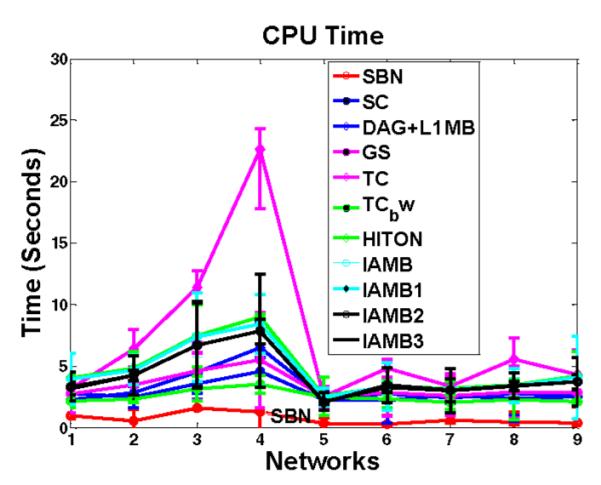
Comparison of SBN with competing algorithms on CPU time in structure learning. Y -axis is the CPU time for each sweep through all the columns of B on a computer with Intel Core 2, 2.2 GHz, 4 GB memory. The X-axis is the first nine networks in Table 1.
Note that the CPU times being compared here do not include the time of initialization and selection of parameters that need to be preset for each algorithm. Inclusion of this time is obviously more desirable for a comprehensive assessment of each algorithm’s efficiency. This, on the other hand, is quite difficult because different algorithms have different initial values and parameters to be preset and there are many different ways to set them. Also, how to set them depends on the requirement for learning accuracy. We leave such a comprehensive assessment and comparison for future study and acknowledge the limitation of the current study.
6 Brain Connectivity Modeling of AD by SBN
FDG-PET images of 49 AD and 67 matching normal control subjects are downloaded from the Alzheimer’s Disease Neuroimaging Initiative website (www.loni.ucla.edu/ADNI). Demographic information and MMSE scores of the subjects are given in Table 3. The ADNI was launched in 2003 by the National Institute on Aging (NIA), the National Institute of Biomedical Imaging andBioengineering (NIBIB), the Food and Drug Administration (FDA), private pharmaceutical companies, and nonprofit organizations as a $60 million, 5-year public-private partnership. The primary goal of ADNI has been to test whether serial MRI, PET, other biological markers, and clinical and neuropsychological assessment can be combined to measure the progression of MCI and early AD.
TABLE 3.
Demographic Information and MMSE
| NC | AD | P-VALUE | |
|---|---|---|---|
| Age (mean ± SD) | 76.0±4.69 | 75.3±6.85 | 0.53 |
| Gender (Male/Female) | 43/24 | 27/22 | 0.77 |
| Years of education (mean ± SD) | 15.9±3.24 | 14.7±3.02 | 0.01 |
| Baseline MMSE | 29.0±1.18 | 23.6±1.93 | <0.001 |
We apply Automated Anatomical Labeling [52] to segment each image into 116 anatomical volumes of interest (AVOIs) and then select 42 AVOIs that are considered to be potentially relevant to AD based on the literature. Each AVOI becomes a region/variable/node in SBN. Please see Table 4 for the name of each AVOI brain region. These regions distributed in the four lobes of the brain, i.e., the frontal, parietal, occipital, and temporal lobes. The measurement data of each region, according to the mechanism of FDG-PET, is the regional average FDG binding counts, representing the degree of glucose metabolism.
TABLE 4.
Names of the AVOI for Brain Connectivity Modeling (L = Left Hemisphere, R = Right Hemisphere)
| Frontal lobe | Parietal lobe | Occipital lobe | Temporal lobe | ||||
|---|---|---|---|---|---|---|---|
| 1 | Front al_Sup_L | 13 | Parietal_Sup_L | 21 | Occipital_Sup_L | 27 | Temporal_Sup_L |
| 2 | Frontal_Sup_R | 14 | Parietal_Sup_R | 22 | Occipital_Sup_R | 28 | Temporal_Sup_R |
| 3 | Frontal_Mid_L | 15 | Parietal_Inf_L | 23 | Occipital_Mid_L | 29 | Temporal_Pole_Sup_L |
| 4 | Frontal_Mid_R | 16 | Parietal_Inf_R | 24 | Occipit al_Mid_R | 30 | Temporal_Pole_Sup_R |
| 5 | Frontal_Sup_Medial_L | 17 | Precuneus_L | 25 | Occipital_Inf_L | 31 | Temporal_Mid_L |
| 6 | Frontal_Sup_Medial_R | 18 | Precuneus_R | 26 | Occipital_Inf_R | 32 | Temporal_Mid_R |
| 7 | Frontal_Mid_Orb_L | 19 | Cingqlum_Post_L | 33 | Temporal_Pole_Mid_L | ||
| 8 | Frontal_Mid_Orb_R | 20 | Cingqlum_Post_R | 34 | Temporal_Pole_Mid_R | ||
| 9 | Rectus_L | 35 | Temporal_Inf_L 8301 | ||||
| 10 | Rectus_R | 36 | Temporal_Inf_R 8302 | ||||
| 11 | Cingulum_Ant_L | 37 | Fusiform_L | ||||
| 12 | Cingulum_Ant_R | 38 | Fusiform_R | ||||
| 39 | Hippocampus_L | ||||||
| 40 | Hippocampus_R | ||||||
| 41 | ParaHippocampal_L | ||||||
| 42 | ParaHippocampal_R | ||||||
We apply SBN to learn a BN for AD and another one for NC to represent their respective brain connectivity models. Note that because BNs are directed graphical models, a connectivity model learned by SBN reveals the directional effects of one brain region over another—called the effective connectivity of the brain [59]. Effective connectivity has been much less studied in the AD literature, while most existing work focuses on the functional connectivity, i.e., the correlations among brain regions. Studies on effective connectivity can greatly complement the existing functional connectivity studies by providing insight into how the correlations are mediated, which may further lead to an understanding of the mechanism underlying the communication among distinct brain regions. In this sense, SBN has the advantage over undirected graphical models of discovering new knowledge about AD.
In the learning of an AD (or NC) effective connectivity model, the value for λ1 needs to be selected. In this paper, we adopt two criteria in selecting λ1: One is to minimize the prediction error of the model and the other is to minimize the BIC. Both criteria have been popularly adopted in sparse learning [20], [21], [22], [37]. The two criteria lead to similar findings from the effective connectivity models, so only the results based on the minimum prediction error are shown in this section and the results based on BIC are included in the supplemental material, which is available online. For a given λ1 value, the prediction error of the corresponding BN is computed as follows: First, a regression is fit for each node using the parents as predictors, and the regression coefficients are estimated by MLE. Then, the mean square error between the true and predicted values of each node is computed based on leave-one-out cross validation. Finally, the mean square errors of all the nodes are summed to represent the prediction error of the BN. The λ1 value that leads to the minimum prediction error is selected; with this λ1, SBN is applied to learn a BN brain connectivity model. Fig. 13 shows the connectivity models for AD and NC. Each model is represented by a “matrix.” Each row/column is one AVOI, Xj. A black cell at the ith row and jth column of the matrix represents that Xi is a parent of Xj. On each matrix, four red cubes are used to highlight the four lobes, i.e., the frontal, parietal, occipital, and temporal lobes, from top-left to bottom-right. The black cells inside each red cube reflect intralobe effective connectivity, whereas the black cells outside the cubes reflect interlobe effective connectivity.
Fig. 13.
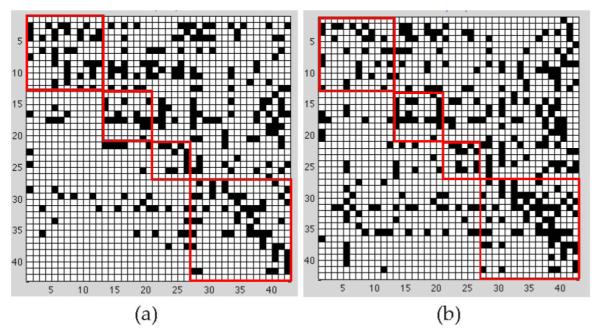
Brain effective connectivity models by SBN. (a) AD; (b) NC.
The following interesting observations can be drawn from the connectivity models.
6.1 Global-Scale Effective Connectivity
The total number of arcs in a BN connectivity model— equal to the number of black cells in a matrix plot in Fig. 13—represents the amount of effective connectivity (i.e., the amount of directional information flow) in the whole brain. This number is 285 and 329 for AD and NC, respectively. In other words, AD has 13.4 percent less amount of effective connectivity than NC. Loss of connectivity in AD has been widely reported in the literature [60], [68], [69], [70].
6.2 Intra/Interlobe Effective Connectivity Distribution
Aside from having different amounts of effective connectivity at the global scale, AD may also have a different distribution pattern of connectivity across the brain from NC. Therefore, we count the number of arcs in each of the four lobes and between each pair of lobes in the AD and NC effective connectivity models. The results are summarized in Table 5. It can be seen that the temporal lobe of AD has 22.9 percent less amount of effective connectivity than NC. The decrease in connectivity in the temporal lobe of AD has been extensively reported in the literature [53], [54], [55]. The interpretation may be that AD is featured by dramatic cognitive decline and the temporal lobe is responsible for delivering memory and other cognitive functions. As a result, the temporal lobe is affected early and severely by AD, and the connectivity network in this lobe is severely disrupted. On the other hand, the frontal lobe of AD has 27.6 percent more amount of connectivity than NC. This observation has been interpreted as compensatory reallocation or recruitment of cognitive resources [56], [53], [57]. Because the regions in the frontal lobe are typically affected later in the course of AD (our data uses mild to moderate AD), the increased connectivity in the frontal lobe may help preserve some cognitive functions in AD patients. In addition, AD shows a decrease in the amount of connectivity in the parietal lobe, which has also been reported to be affected by AD. There is no significant difference between AD and NC in the occipital lobe. This observation is reasonable because the occipital lobe is primarily involved in the brain’s visual function, which is not affected by AD.
TABLE 5.
Intra and Interlobe Effective Connectivity Amounts
| (A) AD | ||||
|---|---|---|---|---|
| Frontal | Parietal | Occipital | Temporal | |
| Frontal | 37 | 28 | 18 | 43 |
| Parietal | 16 | 14 | 42 | |
| Occipital | 10 | 23 | ||
| Temporal | 54 | |||
| (B) NC | ||||
|---|---|---|---|---|
| Frontal | Parietal | Occipital | Temporal | |
| Frontal | 29 | 32 | 12 | 61 |
| Parietal | 20 | 16 | 42 | |
| Occipital | 11 | 36 | ||
| Temporal | 70 | |||
In addition to generating the connectivity models of AD and NC based on the minimum prediction error and minimum BIC criteria, we also generate the connectivity models by making the total numbers of arcs the same for AD and NC. We choose to do this to factor out the connectivity difference between AD and NC that is due to the difference at the global scale so that the remaining difference will reflect their difference in connectivity distribution. Specifically, the connectivity models with the total number of arcs equal to 120, 80, and 60 are generated (see the supplemental material, which is available online), which show similar intra and interlobe effective connectivity distribution patterns to those discussed previously.
6.3 Direction of Local Effective Connectivity
As mentioned previously, one advantage of BNs over undirected graphical models in brain connectivity modeling is that the directed arcs in a BN reflect the directional effect of one region over another, i.e., the effective connectivity. Specifically, if there is a directed arc from brain regions Xi to Xj, it indicates that Xi takes a dominant role in the communication with Xj. The connectivity modes in Fig. 13 reveal a number of interesting findings in this regard.
There are substantially fewer black cells in the area defined by rows 27-42 and columns 1-26 in AD than NC. Recall that rows 27-42 correspond to regions in the temporal lobe. Thus, this pattern indicates a substantial reduction in arcs pointing from temporal regions to the other regions in the AD brain, i.e., temporal regions lose their dominating roles in communicating information with the other regions as a result of AD. The loss is the most severe in the communication from the temporal to frontal regions.
Rows 31 and 35, corresponding to brain regions “Temporal_Mid_L” and “Temporal_Inf_L”, respectively, are among the rows with the largest number black cells in NC, i.e., these two regions take a significantly dominant role in communicating with other regions in normal brains. However, the dominancy of the two regions is substantially reduced by 34.8 and 36.8 percent, respectively, in AD. A possible interpretation is that these are neocortical regions associated with amyloid deposition and early FDG hypometabolism in AD [60], [61], [62], [63], [64], [65].
Columns 39 and 40 correspond to regions “Hippo-campus_L” and “Hippocampus_R,” respectively. There are a total of 33 black cells in these two columns in NC, i.e., 33 other regions dominantly communicate information with the hippocampus. However, this number reduces to 22 (33.3 percent reduction) in AD. The reduction is more severe in Hippocampus_L—actually a 50 percent reduction. The hippocampus is well known to play a prominent role in making new memories and recalling. It has been widely reported that the hippocampus is affected early in the course of AD, leading to memory loss—the most common symptom of AD.
There are a total of 93 arcs pointing from the left to the right hemispheres of the brain in NC; this number reduces to 71 (23.7 percent reduction) in AD. The number of arcs from the right to the left hemispheres in AD is close to that in NC. This provides evidence that AD may be associated with interhemispheric disconnection and the disconnection is mostly unilateral, which has also been reported by some other papers [66], [67].
Finally, we would like to point out that although using BNs to infer effective connectivity is common in the AD literature, it would be more appropriate to study effective connectivity based on PDAGs due to the statistical equivalence of BNs. Therefore, we derive the PDAGs for the DAGs in Fig. 13 (see Fig. S-3 in the supplemental material, which is available online), which turn out to be very similar to the DAGs. We also verify that all the above findings hold based on the PDAGs.
7 Conclusion
In this paper, we proposed a BN structure learning algorithm, SBN, for learning large-scale BN structures from high-dimensional data. SBN adopted a novel formulation that involves one L1-norm penalty term to impose sparsity on the learning and another penalty to ensure the learned BN to be a DAG. We studied the theoretical property of the formulation and identified a finite value for the regularization parameter of the second penalty; this value ensures that the learned BN is a DAG. Under this formulation, we further proposed use of the BCD and shooting algorithms to estimate the BN structure.
Our theoretical analysis on the time complexity of SBN showed that it is linear in the sample size and quadratic in the number of variables. This makes SBN more scalable and efficient than most existing algorithms, and thus makes it well suited for large-scale BN structure learning from high-dimensional datasets. In addition, we performed theoretical analysis on the competitive advantage of SBN over the existing algorithms in terms of learning accuracy. Our analysis showed that the existing algorithms employ a two-stage approach in BN structure identification, and thus having a high risk of misidentifying parents of each variable, whereas SBN does not suffer from this problem.
Our experiments on 11 moderate to large benchmark networks showed that SBN outperforms 10 competing algorithms in all metrics defined for measuring the learning accuracy and under various sample sizes. Also, SBN outperforms the 10 competing algorithms in scalability and efficiency.
We applied SBN to identify the effective brain connectivity model of AD from neuroimaging PDG-PET data. Compared with a brain connectivity model of NC, we found that AD had significantly reduced amounts of effective connectivity in key pathological regions. This is consistent with known pathology and the clinical progression in AD. Clinically, our findings may be useful for monitoring disease progress, evaluating treatment effects (both symptomatic and disease modifying), and enabling early detection of network disconnection in prodromal AD.
In future work, we will investigate how to measure statistical significance of the DAG identified by our algorithm. Potential methods include bootstrap [71], permutation tests [72], and stability selection [73]. This study is also important from the medical point of view as it will help verify the significance of the identified brain connectivity loss based on the DAG. Also, although this paper focuses on structure learning of Gaussian BNs, the same formulation may be adopted for discrete BNs, which will be interesting to explore. In addition, we will investigate the behavior of SBN on Markov equivalent class. Our empirical observation has shown that the objective function of SBN is not Markov equivalent, i.e., SBN attributes different scores to BNs that are Markov equivalent. More in-depth theoretical analysis will be performed in future research.
Supplementary Material
ACKNOWLEDGMENTS
This material is based in part on work supported by the US National Science Foundation under Grant No. CMMI-0825827, CMMI-1069246, MCB-1026710, and the National Institutes of Health under Grant No. 1ROIGM096194-01. Data collection and sharing for this project were funded by the Alzheimer’s Disease Neuroimaging Initiative (ADNI; Principal Investigator: Michael Weiner; NIH grant U01 AG024904). ADNI is funded byt he National Institute on Aging, the National Institute of Biomedical Imaging and Bioengineering (NIBIB), and through generous contributions from the following: Pfizer Inc., Wyeth Research, Bristol-Myers Squibb, Eli Lilly and Company, GlaxoS-mithKline, Merck & Co. Inc., AstraZeneca AB, Novartis Pharmaceuticals Corporation, Alzheimer’sAssociation, Eisai Global Clinical Development, Elan Corporation plc, Forest Laboratories, and the Institute for the Study of Aging, with participation from the US Food and Drug Administration. Industry partnerships are coordinated through the Foundation for the National Institutes of Health. The grantee organization is the Northern California Institute for Research and Education, and the study is coordinated by the Alzheimer’s Disease Cooperative Study at the University of California, San Diego. ADNI data are disseminated by the Laboratory of Neuro Imaging at the University of California, Los Angeles.
Biography
Shuai Huang received the bachelor’s degree in statistics from the University of Science and Technology of China in 2007. Currently, he is working toward the PhD degree in the School of Computing, Informatics, and Decision Systems Engineering at Arizona State University (ASU). His research interests include data mining and machine learning with applications in health and manufacturing. One of his papers was selected as a Feature Article by IIE Magazine.
Jing Li received the PhD degree in industrial and operations engineering from the University of Michigan in 2007. Currently, she is an assistant professor in industrial engineering in the School of Computing, Informatics, and Decision Systems Engineering, Arizona State University. Her research interests include data mining, machine learning, and bioinformatics. She was a recipient of the Best Paper Award from the Institute of Industrial Engineers (IIE) Annual Conference (twice). Two of her papers were selected as Feature Articles by IIE Magazine.
Jieping Ye received the PhD degree in computer science from the University of Minnesota, Twin Cities, in 2005. He is an associate professor ini the Department of Computer Science and Engineering at Arizona State University (ASU). His research interests include machine learning, data mining, and biomedical informatics. He won the outstanding student paper award at ICML in 2004, the SCI Young Investigator of the Year Award at ASU in 2007, the SCI Researcher of the Year Award at ASU in 2009, the US National Secience Foundation Career Award in 2010, and the KDD Best Research Paper Award honorable mention in 2010.

Adam Fleisher received the MD degree from the University of California, San Diego. He is an associate director of brain imaging for the Banner Alzheimer’s Institute (BAI), medical director for the Alzheimer’s Disease Cooperative Study, and an associate professor, Department of Neurosciences, University of California, San Diego. He is recognized for his contributions to the literature in brain imaging of individuals at increased risk for Alzheimer’s Disease (AD), utilizing various volumetric and functional MRI and PET techniques. He has expertise in both neuroimaging and multicenter clinical trials in AD, with a clinical specialty in geriatric neurology, evaluating patients at the BAI Memory Disorders Clinic.

Kewei Chen received the PhD degree in biomathematics from the University of California, Los Angeles, in 1991. Currently, he is a senior scientist and director of the computational image analysis program, Banner Alzheimer Institute (BAI). He also holds adjunct professorships at Arizona State University (ASU), Beijing Normal University, and Shanghai Jiaotong University. His research interests include neuroimage data analysis, processing, multivariate analysis, and radioactive PET tracer kinetic modeling. He has published in the fields of Alzheimer’s neuroimaging studies, on normal human brain functions, and methods in processing neuroimaging data.
Teresa Wu is an associate professor in the industrial engineering program at the School of Computing, Informatics, Decision Systems Engineering, Arizona State University (ASU). Her research interests include distributed decision support and healthcare informatics. Her papers in healthcare informatics have appeared in NeuroImage, the Journal of Digital Image, and RadioGraphics.

Eric Reiman received the MD degree from Duke University. He is an executive director of the Banner Alzheimer’s Institute (BAI), chief scientific officer at the Banner Research Institute, clinical director of the Neurogenomics Division at the Translational Genomics Research Institute (TGen), professor and associate head of Psychiatry at the University of Arizona, and director of the NIA and state-supported Arizona Alzheimer’s Consortium. His research interests include brain imaging, genomics, the presymptomatic detection, tracking and scientific study of Alzheimer’s Disease (AD), the accelerated evaluation of presymptomatic AD treatments using brain imaging and other biomarker methods, and the development of methods with improved power to address these and other objectives.
Footnotes
Data used in preparation of this paper were obtained from the Alzheimer’s Disease Neuroimaging Initiative (ADNI) database (adni.loni.ucla.edu). As such, the investigators within the ADNI contributed to the design and implementation of ADNI and/or provided data but did not participate in the analysis or writing of this report. A complete listing of ADNI investigators can be found at: http://adni.loni.ucla.edu/wp-content/uploads/how_to_apply/ADNI_Acknowledgement_List.pdf.
Contributor Information
Shuai Huang, School of Computing, Informatics, and Decision Systems Engineering, Arizona State University, PO Box 878809, Tempe, AZ 85287-8809..
Jing Li, School of Computing, Informatics, and Decision Systems Engineering, Arizona State University, PO Box 878809, Tempe, AZ 85287-8809. jinglz@asu.edu.
Jieping Ye, School of Computing, Informatics, and Decision Systems Engineering, Arizona State University, PO Box 878809, Tempe, AZ 85287-8809..
Adam Fleisher, Banner Alzheimer’s Institute, 1111 E. McDowell Road, Phoenix AZ 85006..
Kewei Chen, Banner Alzheimer’s Institute, 1111 E. McDowell Road, Phoenix AZ 85006..
Teresa Wu, School of Computing, Informatics, and Decision Systems Engineering, Arizona State University, PO Box 878809, Tempe, AZ 85287-8809..
Eric Reiman, Banner Alzheimer’s Institute, 1111 E. McDowell Road, Phoenix AZ 85006..
References
- [1].Friedman N, Linial M, Nachman I, Péer D. Using Bayesian Networks to Analyze Expression Data. J. Computational Biology. 2000;vol. 7:601–620. doi: 10.1089/106652700750050961. [DOI] [PubMed] [Google Scholar]
- [2].Rodin AS, Boerwinkle E. Mining Genetic Epidemiology Data with Bayesian Networks I: Bayesian Networks and Example Application (Plasma apoE Levels) Bioinformatics. 2005;vol. 21(no. 15):3273–3278. doi: 10.1093/bioinformatics/bti505. [DOI] [PMC free article] [PubMed] [Google Scholar]
- [3].Marcot BG, Holthausen RS, Raphael MG, Rowland M, Wisdom M. Using Bayesian Belief Networks to Evaluate Fish and Wildlife Population Viability under Land Management Alternatives from an Environmental Impact Statement. Forest Ecology and Management. 2001;vol. 153(nos. 1-3):29–42. [Google Scholar]
- [4].Borsuk ME, Stow CA, Reckhow KH. A Bayesian Network of Eutrophication Models for Synthesis, Prediction, and Uncertainty Analysis. Ecological Modelling. 2004;vol. 173:219–239. [Google Scholar]
- [5].Dai H, Korb KB, Wallace CS, Wu X. A Study of Casual Discovery with Weak Links and Small Samples. Proc. 15th Int’l Joint Conf. Artificial Intelligence.1997. pp. 1304–1309. [Google Scholar]
- [6].Mani S, Cooper GF. A Study in Casual Discovery from Population-Based Infant Birth and Death Records. Proc. AMIA Ann. Fall Symp. 1999:315–319. [PMC free article] [PubMed] [Google Scholar]
- [7].Rajapakse JC, Zhou J. Learning Effective Brain Connectivity with Dynamic Bayesian Networks. NeuroImage. 2007;vol. 37:749–760. doi: 10.1016/j.neuroimage.2007.06.003. [DOI] [PubMed] [Google Scholar]
- [8].Li JN, Wang ZJ, Palmer SJ, McKeown MJ. Dynamic Bayesian Network Modeling of fMRI: A Comparison of Group-Analysis Methods. NeuroImage. 2008;vol. 37:749–760. doi: 10.1016/j.neuroimage.2008.01.068. [DOI] [PubMed] [Google Scholar]
- [9].Li J, Shi J. Knowledge Discovery from Observational Data for Process Control through Causal Bayesian Networks. IIE Trans. 2007;vol. 39(no. 6):681–690. [Google Scholar]
- [10].De Campos L. Independency Relationships and Learning Algorithms for Singly Connected Networks. J. Experimental and Theoretical Artificial Intelligence. 1998;vol. 10:511–549. [Google Scholar]
- [11].De Campos L, Huete J. A New Approach for Learning Belief Networks Using Independence Criteria. Int’l J. Approximate Reasoning. 2000;vol. 24:11–37. [Google Scholar]
- [12].Pearl J, Verma T. Equivalence and Synthesis of Causal Models. Proc. Sixth Conf. Uncertainty in Artificial Intelligence.1990. [Google Scholar]
- [13].Spirtes P, Glymour C, Scheines R. Causation, Prediction and Search. Springer; 1993. [Google Scholar]
- [14].Meek C. Causal Inference and Causal Explanation with Background Knowledge. Proc. 11th Conf. Uncertainty in Artificial Intelligence.1995. [Google Scholar]
- [15].Cooper G, Herskovits E. A Bayesian Method for the Induction of Probabilistic Networks from Data. Machine Learning. 1992;vol. 9:309–347. [Google Scholar]
- [16].Heckerman D, Geiger D, Chickering D. Learning Bayesian Networks: The Combination of Knowledge and Statistical Data. Machine Learning. 1995;vol. 20:197–243. [Google Scholar]
- [17].Buntine W. A Guide to the Literature on Learning Probabilistic Networks from Data. IEEE Trans. Knowledge and Data Eng. 1996 Apr.vol. 8(no. 2):195–210. [Google Scholar]
- [18].Friedman N, Koller D. Being Bayesian about Network Structure: A Bayesian Approach to Structure Discovery in Bayesian Networks. Machine Learning. 2003;vol. 50:95–125. [Google Scholar]
- [19].Heckerman D. A Tutorial on Learning Bayesian Networks. Microsoft Research; 1996. Technical Report MSR-TR-95-06. [Google Scholar]
- [20].Lam W, Bacchus F. Learning Bayesian Belief Networks, an Approach Based on the MDL Principle. Computational Intelligence. 1994;vol. 10:269–293. [Google Scholar]
- [21].Suzuki JA. Construction of Bayesian Networks from Databases Based on an MDL Principle. Proc. Ninth Conf; Uncertainty in Artificial Intelligence; 1993. pp. 266–273. [Google Scholar]
- [22].Bouckaert R. Symbolic and Quantitative Approaches to Reasoning and Uncertainty. Springer; 1993. Belief Networks Construction Using the Minimum Description Length Principle; pp. 41–48. [Google Scholar]
- [23].Friedman N, Goldszmidt M. Learning Bayesian Networks with Local Structure. Proc. 12th Conf; Uncertainty in Artificial Intelligence; 1996. [Google Scholar]
- [24].Chow C, Liu C. Approximating Discrete Probability Distributions with Dependence Trees. IEEE Trans. Information Theory. 1968 May;vol. 14(no. 3):462–467. [Google Scholar]
- [25].Chickering D. Optimal Structure Identification with Greedy Search. J. Machine Learning Research. 2002;vol. 3:507–554. [Google Scholar]
- [26].Acid S, De Campos J. Searching for Bayesian Network Structures in the Space of Restricted Acyclic Partially Directed Graphs. J. Artificial Intelligence Research. 2003;vol. 18:445–490. [Google Scholar]
- [27].Castelo R, Kocka T. On Inclusion-Driven Learning of Bayesian Networks. J. Machine Learning Research. 2003;vol. 4:527–574. [Google Scholar]
- [28].Larranaga R, Kuijpers C, Murga R, Yurramendi Y. Learning Bayesian Network Structures by Searching for the Best Ordering with Genetic Algorithms. IEEE Trans. Systems, Man, and Cybernetics. 1996 Jul;vol. 26(no. 4):487–493. [Google Scholar]
- [29].Larranaga P, Poza M, Yurramendi Y, Murga R, Kuijpers C. Structure Learning of Bayesian Networks by Genetic Algorithms: A Performance Analysis of Control Parameters. IEEE Trans. Pattern Analysis and Machine Intelligence. 1996 Sept.vol. 18(no. 9):912–926. [Google Scholar]
- [30].Chickering D, Geiger D, Heckerman D. Learning Bayesian Networks: Search Methods and Experimental Results. Proc. Preliminary Papers Fifth Int’l Workshop Artificial Intelligence and Statistics.1995. [Google Scholar]
- [31].Chen XW, Anantha G, Lin XT. Improving Bayesian Network Structure Learning with Mutual Information-Based Node Ordering in the K2 Algorithm. IEEE Trans. Knowledge and Data Eng. 2008 May;vol. 20(no. 5):628–640. [Google Scholar]
- [32].Hoyer PO, Janzing D, Mooij JM, Peters J, Scholkopf B. Nonlinear Causal Discovery with Additive Noise Models. Proc. Conf. Neural Information Processing Systems.2009. [Google Scholar]
- [33].Peng J, Wang P, Zhou N, Zhu J. Partial Correlation Estimation by Joint Sparse Regression Models. J. Am. Statistical Assoc. 2009;vol. 104:735–746. doi: 10.1198/jasa.2009.0126. [DOI] [PMC free article] [PubMed] [Google Scholar]
- [34].Sporns O, Chialvo DR, Kaiser M, Hilgetag CC. Organization, Development and Function of Complex Brain Networks. Trends in Cognitive Sciences. 2004;vol. 8:418–425. doi: 10.1016/j.tics.2004.07.008. [DOI] [PubMed] [Google Scholar]
- [35].Friedman N, Nachman I, Péer D. Learning Bayesian Network Structure from Massive Datasets: The ‘Sparse Candidate’ Algorithm. Proc. 15th Conf. Uncertainty in Artificial Intelligence.1999. [Google Scholar]
- [36].Schmidt M, Niculescu-Mizil A, Murphy K. Learning Graphical Model Structures using L1-Regularization Paths. Proc. 22nd Nat’l Conf. Artificial Intelligence.2007. [Google Scholar]
- [37].Tibshirani R. Regression Shrinkage and Selection via the Lasso. J. Royal Statistical Soc. Series B. 1996;vol. 58(no. 1):267–288. [Google Scholar]
- [38].Tsamardinos I, Brown LE, Aliferis CF. The Max-Min Hill-Climbing Bayesian Network Structure Learning Algorithm. Machine Learning. 2006;vol. 65(no. 1):31–78. [Google Scholar]
- [39].Margaritis D, Thrun S. Bayesian Network Induction via Local Neighborhoods. Proc. Conf. Advances in Neural Information Processing Systems.1999. [Google Scholar]
- [40].Pellet JP, Elisseeff A. Using Markov Blankets for Causal Structure Learning. J. Machine Learning Research. 2008;vol. 9:1295–1342. [Google Scholar]
- [41].Estrada E, Naomichi H. Communicability in Complex Networks. Physics Rev. E. 2008;vol. 77:036111. doi: 10.1103/PhysRevE.77.036111. [DOI] [PubMed] [Google Scholar]
- [42].Luus R, Wyrwicz R. Use of Penalty Functions in Direct Search Optimization. Hungarian J. Industrial Chemistry. 1996;vol. 24:273–278. [Google Scholar]
- [43].Bertsekas DP. Nonlinear Programming. second ed Athena Scientific; 1999. [Google Scholar]
- [44].Fu W. Penalized Regressions: The Bridge vs the Lasso. J. Computational and Graphical Statistics. 1998;vol. 7(no. 3):397–416. [Google Scholar]
- [45].Cormen TH, Leiserson CE, Rivest RL, Stein C. Introduction to Algorithms. third ed MIT Press; 2001. [Google Scholar]
- [46].Friedman J, Hastie T, Hofling H, Tibshirani R. Pathwise Coordinate Optimization. The Annals of Applied Statistics. 2007;vol. 1(no.2):302–332. [Google Scholar]
- [47].Aliferis CF, Tsamardinos I, Statnikov A. HITON, a Novel Markov Blanket Algorithm for Optimal Variable Selection. Proc. AMIA Ann. Symp.; 2003. [PMC free article] [PubMed] [Google Scholar]
- [48].Tsamardinos I, Aliferis C. Towards Principled Feature Selection: Relevancy, Filters and Wrappers. Proc. Ninth Int’l Workshop Artificial Intelligence and Statistics.2003. [Google Scholar]
- [49].Bayesian Network Repository. 2011 http://www.cs.huji.ac.il/labs/compbio/Repository.
- [50].Tsamardinos I, Statnikov A, Brown LE, Aliferis CF. Generating Realistic Large Bayesian Networks by Tiling. Proc. 19th Int’l FLAIRS Conf..2006. [Google Scholar]
- [51].Mackey D. Information Theory, Inference, and Learning Algorithms. Cambridge Univ. Press; 2003. [Google Scholar]
- [52].Tzourio-Mazoyer N. Automated Anatomical Labelling of Activations in SPM Using a Macroscopic Anatomical Parcellation of the MNI MRI Single Subject Brain. NeuroImage. 2002;vol. 15:273–289. doi: 10.1006/nimg.2001.0978. [DOI] [PubMed] [Google Scholar]
- [53].Supekar K, Menon V, Rubin D, Musen M, Greicius MD. Network Analysis of Intrinsic Functional Brain Connectivity in Alzheimer’s Disease. PLoS Computational Biology. 2008;vol. 4(no. 6):1–11. doi: 10.1371/journal.pcbi.1000100. [DOI] [PMC free article] [PubMed] [Google Scholar]
- [54].Azari NP, Rapoport SI, Grady CL, Schapiro MB, Salerno JA, Gonzales-Aviles A. Patterns of Interregional Correlations of Cerebral Glucose Metabolic Rates in Patients with Dementia of the Alzheimer Type. Neurodegeneration. 1992;vol. 1:101–111. [Google Scholar]
- [55].Wang K, Liang M, Wang L, Tian L, Zhang X, Jiang T. Altered Functional Connectivity in Early Alzheimer’s Disease: A Resting-State fMRI Study. Human Brain Mapping. 2007;vol. 28:967–978. doi: 10.1002/hbm.20324. [DOI] [PMC free article] [PubMed] [Google Scholar]
- [56].Gould RL, Arroyo B, Brown RG, Owen AM, Howard RJ. Brain Mechanisms of Successful Compensation during Learning in Alzheimer Disease. Neurology. 2006;vol. 67:1011–1017. doi: 10.1212/01.wnl.0000237534.31734.1b. [DOI] [PubMed] [Google Scholar]
- [57].Stern Y. Cognitive Reserve and Alzheimer Disease. Alzheimer Disease Associated Disorder. 2006;vol. 20:69–74. doi: 10.1097/01.wad.0000213815.20177.19. [DOI] [PubMed] [Google Scholar]
- [58].Korb KB, Nicholson AE. Bayesian Artificial Intelligence. Chapman & Hall/CRC; 2003. [Google Scholar]
- [59].Friston KJ. Functional and Effective Connectivity in Neuroimaging: A Synthesis. Human Brain Mapping. 1994;vol. 2:56–78. [Google Scholar]
- [60].Greicius MD, Srivastava G, Reiss AL, Menon V. Default-Mode Network Activity Distinguishes AD from Healthy Aging: Evidence from Functional MRI. Proc. Nat’l Academy Sciences USA. 2004;vol. 101:4637–4642. doi: 10.1073/pnas.0308627101. [DOI] [PMC free article] [PubMed] [Google Scholar]
- [61].Alexander GE, Chen K, Pietrini P, Rapoport SI, Reiman EM. Longitudinal PET Evaluation of Cerebral Metabolic Decline in Dementia: A Potential Outcome Measure in Alzheimer’s Disease Treatment Studies. Am. J. Psychiatry. 2002;vol. 159:738–745. doi: 10.1176/appi.ajp.159.5.738. [DOI] [PubMed] [Google Scholar]
- [62].Braak H, Braak E. Evolution of the Neuropathology of Alzheimer’s Disease. Acta Neurologica Scandinavica Supplementum. 1996;vol. 165:3–12. doi: 10.1111/j.1600-0404.1996.tb05866.x. [DOI] [PubMed] [Google Scholar]
- [63].Braak H, Braak E, Bohl J. Staging of Alzheimer-Related Cortical Destruction. European Neurology. 1993;vol. 33:403–408. doi: 10.1159/000116984. [DOI] [PubMed] [Google Scholar]
- [64].Ikonomovic MD, Klunk WE, Abrahamson EE, Mathis CA, Price JC, Tsopelas ND, Lopresti BJ, Ziolko S, Bi W, Paljug WR, Debnath ML, Hope CE, Isanski BA, Hamilton RL, DeKosky ST. Post-Mortem Correlates of In Vivo PiB-PET Amyloid Imaging in a Typical Case of Alzheimer’s Disease. Brain. 2008;vol. 131:1630–1645. doi: 10.1093/brain/awn016. [DOI] [PMC free article] [PubMed] [Google Scholar]
- [65].Klunk WE, Engler H, Nordberg A, Wang Y, Blomqvist G, Holt DP, Bergstrom M, Savitcheva I, Huang GF, Estrada S, Ausen B, Debnath ML, Barletta J, Price JC, Sandell J, Lopresti BJ, Wall A, Koivisto P, Antoni G, Mathis CA, Langstrom B. Imaging Brain Amyloid in Alzheimer’s Disease with Pittsburgh Compound-B. Annals of Neurology. 2004;vol. 55:306–319. doi: 10.1002/ana.20009. [DOI] [PubMed] [Google Scholar]
- [66].Reuter-Lorenz PA, Mikels JA. A Split-Brain Model of Alzheimer’s Disease? Behavioral Evidence for Comparable Intra and Interhemispheric Decline. Neuropscyhologia. 2005;vol. 43:1307–1317. doi: 10.1016/j.neuropsychologia.2004.12.007. [DOI] [PubMed] [Google Scholar]
- [67].Lipton AM, Benavides R, Hynan LS, Bonte FJ, Harris TS, White CL, III, Bigio EH. Lateralization on Neuroimaging Does Not Differentiate Frontotemporal Lobar Degeneration from Alzheimer’s Disease. Dementia and Geriatric Cognitive Disorders. 2004;vol. 17(no. 4):324–327. doi: 10.1159/000077164. [DOI] [PubMed] [Google Scholar]
- [68].Hedden T, Van Dijk KR, et al. Disruption of Functional Connectivity in Clinically Normal Older Adults Harboring Amyloid Burden. J. Neuroscience. 2009;vol. 29:12686–12694. doi: 10.1523/JNEUROSCI.3189-09.2009. [DOI] [PMC free article] [PubMed] [Google Scholar]
- [69].Andrews-Hanna JR, et al. Disruption of Large-Scale Brain Systems in Advanced Aging. Neuron. 2007;vol. 56:924–935. doi: 10.1016/j.neuron.2007.10.038. [DOI] [PMC free article] [PubMed] [Google Scholar]
- [70].Wu X, Li R, Fleisher AS, Reiman EM, Chen K, Yao L. Altered Default Mode Network Connectivity in AD—A Resting Functional MRI and Bayesian Network Study. Human Brain Mapping. 2011;vol. 32:1868–1881. doi: 10.1002/hbm.21153. [DOI] [PMC free article] [PubMed] [Google Scholar]
- [71].Efron B, Ribshirani RJ. An Introduction to the Bootstrap. CRC Press; 1994. [Google Scholar]
- [72].Good P. Permutation, Parametric and Bootstrap Tests of Hypotheses. third ed Springer; 2005. [Google Scholar]
- [73].Meinshausen N, Buehlmann P. Stability Selection. J. Royal Statistical Soc., Series B. 2010;vol. 72:417–473. [Google Scholar]
Associated Data
This section collects any data citations, data availability statements, or supplementary materials included in this article.