MNE software for processing MEG and EEG data

Abstract

Magnetoencephalography and electroencephalography (M/EEG) measure the weak electromagnetic signals originating from neural currents in the brain. Using these signals to characterize and locate brain activity is a challenging task, as evidenced by several decades of methodological contributions. MNE, whose name stems from its capability to compute cortically-constrained minimum-norm current estimates from M/EEG data, is a software package that provides comprehensive analysis tools and workflows including preprocessing, source estimation, time–frequency analysis, statistical analysis, and several methods to estimate functional connectivity between distributed brain regions. The present paper gives detailed information about the MNE package and describes typical use cases while also warning about potential caveats in analysis. The MNE package is a collaborative effort of multiple institutes striving to implement and share best methods and to facilitate distribution of analysis pipelines to advance reproducibility of research. Full documentation is available at http://martinos.org/mne.

1. Introduction

By non-invasively measuring electromagnetic signals ensuing from neurons, M/EEG are unique tools to investigate the dynamically changing patterns of brain activity. Functional magnetic resonance imaging (fMRI) provides a spatial resolution in the millimeter scale, but its temporal resolution is limited as it measures neuronal activity indirectly by imaging the slow hemodynamic response. On the other hand, EEG and MEG measure the electric and magnetic fields directly related to the underlying electrophysiological processes and can thus attain a high temporal resolution. This enables the investigation of neuronal activity over a wide range of frequencies. High-frequency oscillations, for example, are thought to play a central role in neuronal computation as well as to serve as the substrate of consciousness and awareness (Fries, 2009; Tallon-Baudry et al., 1997). Low-frequency modulations, some of them possibly associated with resting-state networks observed with fMRI, can also be successfully captured with MEG (Brookes et al., 2011; Hipp et al., 2012).

However, the processing of M/EEG data to obtain accurate localization of active neural sources is a complicated task: it involves segmenting various structures from anatomical MRIs, numerical solution of the electromagnetic forward problem, signal denoising, a solution to the ill-posed electromagnetic inverse problem, and appropriate control of multiple statistical comparisons spanning space, time and frequency across experimental conditions and groups of subjects. This complexity not only constitutes a challenge to MEG investigators but also offers a great deal of flexibility in data analysis. To successfully process M/EEG data, comprehensive and well-documented analysis software is therefore required.

MNE is an academic software package that aims to provide data analysis pipelines encompassing all phases of M/EEG data processing. Multiple academic software packages for M/EEG data processing exist, e.g., Brainstorm (Tadel et al., 2011), EEGLAB (Delorme and Makeig, 2004; Delorme et al., 2011), Field-Trip (Oostenveld et al., 2011), NutMeg (Dalal et al., 2011) and SPM (Litvak et al., 2011), all implemented in Matlab, with some dependencies on external packages such as OpenMEEG (Gramfort et al., 2010) for boundary element method (BEM) forward modeling or NeuroFEM for volume based finite element method (FEM) (Wolters et al., 2007) forward modeling. Many analysis methods are common to all these packages, yet MNE has some unique capabilities. Among these are a tight integration with the anatomical reconstruction provided by the FreeSurfer software, as well as a selection of inverse solvers for source imaging.

MNE software consists of three core subpackages which are fully integrated: the original MNE-C (distributed as compiled C code), MNE-Matlab, and MNE-Python. The subpackages employ the same Neuromag FIF file format and use consistent analysis steps with compatible intermediate files. Consequently, the packages can be combined for a particular task in a flexible manner. The FIF file format allows storage of any type of information in a single file using a hierarchy of elements known as tags. The original MNE-C, conceived and written at the Martinos Center at Massachusetts General Hospital, consists of command line programs that can be used in shell scripts for automated processing, and two graphical user interface (GUI) applications for raw data inspection, coordinate alignment, and inverse modeling, as illustrated in Fig 1. MNE-C is complemented by two more recent software packages, MNE-Matlab and MNE-Python. Both are open source and distributed under the simplified BSD license allowing their use in free as well as in commercial software.

Figure 1.

Graphical user interface (GUI) applications provided by MNE-C. Top: mne_analyze for coordinate alignment and inverse modeling. Bottom: mne browse raw for raw data inspection and processing.

The MNE-Matlab code provides basic routines for reading and writing FIF files. It is redistributed as a part of several Matlab-based M/EEG software packages (Brainstorm, FieldTrip, NutMeg, and SPM). The MNE-Python code is the most recent addition to the MNE software; it started as a reimplementation of the MNE-Matlab code, removing any dependencies on commercial software. After an intensive collaborative software development effort, MNE-Python now provides several additional features, such as time–frequency analysis, non-parametric statistics, and connectivity estimation. An overview of the analysis components supported by the various parts of MNE is shown in Table 1. The comprehensive set of features offered by the Python package is made possible by a group of dedicated contributors at multiple institutions in several countries who collaborate closely. This is facilitated by the use of a software development process that is entirely public and open for anyone to contribute.

Table 1.

Overview of the features provided by the command-line tools and the compiled GUI applications (MNE-C) and the MNE-Matlab and MNE-Python toolboxes (✓: supported). All parts of MNE read and write data in the same file format, enabling users to use the tool that is best suited for each processing step. ECD = Equivalent Current Dipole; LCMV = Linearly Constrained Minimum-Variance

Processing module	MNE-C	MNE-Matlab	MNE-Python
Filtering	✓		✓
Signal space projection (SSP)	✓	✓	✓
Indep. component analysis (ICA)			✓
Coregistration of MEG and MRI	✓		✓
Forward modeling	✓
Time–frequency analysis			✓
Dipole modeling (ECD)	✓
Minimum-norm estimation (ℓ2)	✓	✓	✓
Mixed-norm estimation (MxNE)			✓
Time–frequency MxNE			✓
Beamforming (LCMV, DICS)			✓
Spatial morphing	✓	✓	✓
Connectivity estimation			✓
Statistics			✓

From a user’s perspective, moving between the components listed in Table 1 means moving between different scripts in a text editor. Using the enhanced interactive IPython shell (Pérez and Granger, 2007), a core ingredient of the standard scientific Python stack, all MNE components can be interactively accessed simultaneously from within one environment. For example, one may enter ‘!mne_analyze’ in the IPython shell to launch the MNE-C GUI to perform coordinate alignment. After closing the GUI, they could return back to the Python session to proceed with the FIF file generated during that step. An extensive set of example scripts exposing typical workflows or elements thereof while serving as copy and paste templates are available on the MNE website and are included in the MNE-Python code.

The MNE software also provides a sample dataset consisting of recordings from one subject with combined M/EEG conducted at the Martinos Center of Massachusetts General Hospital. These data were acquired with a Neuromag VectorView system (Elekta Oy, Helsinki, Finland) with 306 sensors arranged in 102 triplets, each comprising two orthogonal planar gradiometers and one magnetometer. EEG were recorded simultaneously using an MEG-compatible cap with 60 electrodes. In the experiment, auditory stimuli (delivered monaurally to the left or right ear), and visual stimuli (shown in the left or right visual hemifield) were presented in a random sequence with a stimulus-onset asynchrony (SOA) of 750 ms. To control for subject’s attention, a smiley face was presented intermittently and the subject was asked to press a button upon its appearance. These data are provided with the MNE-Python package and they are used in this paper for illustration purposes. This dataset can also serve as a standard validation dataset for M/EEG methods, hence favoring reproducibility of results. However, induced responses, recovered by time–frequency analysis, are illustrated in the present paper using somatosensory responses to electric stimulation of the median nerve at wrist. These data (see (Sorrentino et al., 2009) for details) were recorded with a similar MEG system as the MNE sample data. In addition to the provided sample data, MNE-Python facilitates easy access to the MEGSIM datasets (Aine et al., 2012) that include both experimental and simulated MEG data. These data are continuous raw signals, single-trial or averaged evoked responses, with either auditory, visual, or somatosensory stimuli presented to the subjects.

The goal of this contribution is to describe the MNE software in detail and to illustrate how to implement good analysis practices (Gross et al., 2013) as MNE pipelines. We also explicitly mention potential caveats in different stages of the analysis. With this work, we aim to help standardize M/EEG analysis pipelines, which will improve the reproducibility of research findings.

The structure of the paper follows the natural order of steps performed when analyzing M/EEG data, from preprocessing to statistical analysis of source estimates, including methods such as time–frequency analysis and functional connectivity estimation. We first present an overview of standard analysis methods before detailing the recommended MNE analysis strategy.

2. Standard M/EEG data analysis components

2.1. Data inspection and de-noising

As the first step of a general M/EEG analysis workflow, the raw data need to be inspected for interference and artifacts, which includes detecting dysfunctional, noisy and “jumping” channels. While the software provided by M/EEG vendors is generally useful for reviewing the data, both MNE-C and MNE-Python offer raw data visualization tools that facilitate the identification of such bad channels. Besides inspecting the raw sensor time courses for artifacts, spatial patterns may add valuable information. These patterns can be displayed at each time instant as a contour map generated from interpolations over channel locations. These kinds of topographic visualizations are especially useful when assembled to movies, such that the dynamics of the magnetic field and potential patterns appearing, disappearing, and reappearing can be better understood. While it is also possible to employ automatic artifact rejection procedures right from the beginning, e.g., using signal space separation (Taulu, 2006), it is a good practice to inspect the data visually at an early stage of processing.

After this initial inspection and removal of bad channels and data segments, it is recommended to apply more formal noise suppression methods. Although it may not always be obvious, the selection of a noise rejection procedure invariably implies some assumptions about the nature of the signals and noise. For MEG data, some procedures correct for sensor and environmental noise by employing a noise-covariance matrix estimated from data acquired in the absence of a subject. Alternatively, a “subject noise” covariance can be estimated from pre-stimulus intervals available in evoked-response studies. If the goal is to study ongoing, task-free, or instantenous single-trial activity, the separation of subject noise from the signal of interest is less plausible. In this case, the conservative choice of employing the empty-room noise-covariance matrix is a safe option. The inverse solution methods discussed later support both options.

2.2. Source localization

After effective noise reduction, sensor-level data may already indicate the probable number and approximate locations of active sources. In order to actually localize such sources, that is, to propose unique solutions to the ill-posed biomagnetic inverse problem, different techniques exist. Each of these techniques has its own modeling assumptions and thus also strengths and limitations. Therefore, the MNE software provides a selection of different inverse modeling approaches. Importantly, in all of these approaches, the elementary source employed is a current dipole, motivated by the physiological nature of the cerebral currents measurable in M/EEG (Hämäläinen et al., 1993). Different source modeling approaches are set apart by the selection of constraints on the sources and other criteria to arrive at the best estimate for the cerebral current distribution as a function of time.

2.2.1. Dipole methods

A classic source localization approach assumes that the signals observed can be explained by a small number of equivalent current dipoles (ECD). In particular, time-varying dipole fitting (Scherg and Von Cramon, 1985), has been very successful in characterizing both basic sensory responses, more complex constellations of sources in cognitive experiments, and abnormal activity, e.g., in epileptic patients. While the resulting models can be compellingly parsimonious and easy to interpret, the assumption of a small set of focal activations is not always warranted given the nature of the neural processes under investigation. For example, complex cognitive tasks and ongoing spontaneous or “resting state” activity is likely to involve multiple brain regions where the spatial extent of the activity may be too large to be properly accounted for by a current dipole. In addition, the use of cortical constraints maybe too restricting for the ECD approach because, unlike in a volumetric model with unrestricted source locations, the dipole may not move freely to best account for extended activations, see, e.g., (Hari, 1991).

2.2.2. Distributed solutions

Some of the problems of multiple dipole fitting, including the reliable estimation of the dipole location parameters, can be overcome by using a distributed source model that simultaneously models a large number of spatially fixed dipoles whose amplitudes are estimated from the data. To solve this highly under-determined problem, one employs a cost function which consists of a least-squares error or “data” term, favoring a solution which explains the (whitened) measured data in the least-squares sense, and a “model term” favoring a particular current distribution. In Bayesian terms, this corresponds to modeling measurement noise as a multivariate Gaussian distribution in combination with a source prior, which can be directly related to the model term in the cost function (Wipf and Nagarajan, 2009). While it is beyond the scope of this paper to discuss the relative merits, drawbacks, and mathematical formulations of the various inverse methods described below (and implemented in MNE), we urge readers to carefully consider the underlying assumptions and technical issues outlined in the publications covering these methods.

One popular source prior is exemplified in the minimum-norm estimates (MNE, Wang et al. 1992; Hämäläinen and Ilmoniemi 1994). In this approach, among all the current distributions that can explain the data equally well, the one with the minimum ℓ₂-norm is favored. This norm yields small, distributed estimates of cerebral currents (compared to e.g., an ℓ₁ norm, which favors a few, large-amplitude currents) to explain the observed sensor data. This MNE approach has subsequently been refined to take into account cortical location and orientation constraints (Lin et al., 2006a), motivated by the neurophysiological knowledge on the primary sources of the MEG and EEG signals. The most significant contributions to the M/EEG signals originate from postsynaptic currents in the pyramidal cells in the cortex and the net direction of these currents is oriented perpendicular to the cortical surface (Dale and Sereno, 1993). Incorporating this knowledge to the model implies using individual anatomical information acquired with structural magnetic resonance imaging (MRI). The current estimates can then be constrained to the cortical mantle while the orientations of the currents can be further restricted to be perpendicular to the local cortical surface (Lin et al., 2006a). To quantify the statistical significance of the current estimates, noise normalization techniques have been developed (Dale et al., 2000; Pascual-Marqui, 2002) yielding a dimensionless statistical score instead of dipole amplitudes in units of Ampere-meter (Am). Mathematically, MNE is closely related to several other inversion approaches (Mosher et al., 2003).

A practical benefit of ℓ₂ solutions is that they yield physiologically plausible, temporally smooth estimates (without discontinuous ‘jumps’). This comes at the cost of giving up some spatial precision. To avoid smeared ℓ₂ estimates, sparsity-promoting priors such as ℓ₁-norm prior may be desirable. Those generate more focal minimum-norm solutions, historically refered to as minimum-current estimates (MCE) (Matsuura and Okabe, 1995; Uutela et al., 1999). Both assets, temporal smoothness and focality, can also be combined using structured norms such as the ℓ₂₁ mixed-norm (Ou et al., 2009; Gramfort et al., 2012). These norms can also be used to model non-stationary activations in the time–frequency domain (Gramfort et al., 2013). The work of Wipf and Nagarajan (2009) offers a unifying view using a Bayesian perspective on some of the solvers implemented in the MNE software such as MNE, sLORETA, and the γ-MAP method.

2.2.3. Beamformers

Another class of distributed approaches, often referred to as scanning methods, is exemplified by so-called adaptive beamformers, such as MUSIC (Mosher and Leahy, 1998), LCMV (Veen et al., 1997), SAM (Robinson and Vrba, 1998), and DICS (Gross et al., 2001). These methods scan a grid of source locations, independently testing each of them for its contribution to the measured signal, similar to a radar beam. Such techniques, some of which are implemented in the MNE software, are almost exclusively computed on volumetric grids, as opposed to cortical surfaces commonly used with MNE. It should be emphasized, however, that even if the results are often referred to as images they should be more appropriately called pseudo images, since they do not represent a distributed estimate of the cerebral electric currents that explain the measured M/EEG. Furthermore, the scanning techniques are most often applied to MEG only, since their efficacy depends on the accuracy of the forward model, which is generally less precise for EEG than for MEG. Moreover, single-source beamformers yield erroneous localizations if several regions exhibit highly correlated activity, which is the case, e.g. for the bilateral auditory evoked responses. However, beamformers have been successfully employed in the analysis of ongoing spontaneous activity, where source correlations are in general so low that the performance of a beamformer does not significantly degrade (Gross et al., 2001). Also, alternative beamformer formulations can alleviate the limitations of single-source beamformers (Wipf and Nagarajan, 2007).

2.3. Statistics

Once activity estimates have been obtained, whether they are on the cortical surface or on a volume grid, a number of statistical measures can be used to determine their significance. This statistical analysis may consider, e.g., significance of activity with respect to a baseline, or differences across hemispheres, between conditions, between subjects, or between subject groups, e.g., patients and normal controls.

Several factors determine which statistical approach is the most appropriate. Parametric methods are widely used and they build on underlying assumptions (typically Gaussian) on the distribution of the data to determine statistical significance, dynamic Statistical Parametric Map (dSPM) estimates of significant activity being one prominent example (Dale et al., 2000). When utilizing parametric methods, it is important to ensure that the underlying model assumptions are satisfied, otherwise the obtained results could be inaccurate (see Pantazis et al. (2005) for discussion).

A more general class of statistical approaches comprises non-parametric methods, which do not rely on assumptions about the distribution of the data. Permutation methods, in particular, exploit the exchangeability of conditions under the null hypothesis to estimate the null distribution by resampling the data (Nichols and Holmes, 2002).

The appropriate statistical treatment depends on many factors, such as whether the neural activity is represented as raw sensor signals, distributed source estimates, or parameters of equivalent current dipoles. Moreover, any given temporal waveform can be represented in terms of frequency content over an entire epoch, or that changes as a function of time. Some analysis choices can increase the apparent dimensionality of the data considerably, and thus attention should be paid to the problem of multiple comparisons. This is a major reason that statistical analysis methods for M/EEG are evolving, and different forms of nonparametric approaches (Nichols and Holmes, 2002; Pantazis et al., 2005), topological considerations (Maris and Oostenveld, 2007), and variance control (Ridgway et al., 2012) are being actively investigated. A comprehensive discussion of the validity of these approaches is beyond the scope of this paper. Our statistical approach outlined below will focus on the relatively new non-parametric cluster-based statistical measures available in MNE, which provide the capability for statistical tests with minimal assumptions about the data distributions.

2.4. Functional connectivity

While the localization of activity using inverse modeling and successive statistical tests can give us information on which brain regions are involved in a task and to what degree the amount of activity depends on other factors, e.g., experimental conditions, such an analysis typically does not reveal how the brain regions relevant to the task are interrelated, apart possibly from the temporal sequence of activity in different regions.

Functional connectivity estimation methods analyze the relationship between a number of time series with the goal of recovering the structure and properties of the network that describes the functional dependencies between the underlying brain regions. Connectivity estimation in M/EEG is typically performed on non-averaged data (often after subtracting the evoked responses from the single trials) in either the sensor or the source space. The latter requires the application of an inverse method to obtain a source estimate for each trial, which is computationally more demanding but has the advantage that the connectivity can more directly be related to the underlying anatomy, which is difficult or even ambiguous for sensor-space connectivity estimates. Connectivity estimation in the sensor space also has the problem that the linear mixing introduced by the forward propagation from cortical currents to the sensors, often referred to as “spatial leakage” or, misleadingly, as “volume conduction”, can have a confounding effect on connectivity estimates. For connectivity analysis, data can be segmented in consecutive epochs, e.g., 1 or 2 s, after filtering. This has the benefit of using the same analysis pipeline used for task-based data, which is particularly convenient as it allows an automatic rejection of corrupted time segments using the epoch rejection mechanisms.

MNE provides functions for connectivity estimation in both the sensor and source space. The supported methods are bivariate spectral measures, i.e., connectivity is estimated by analyzing pairs of time series, and they depend on the phase consistency across epochs between the time series at a given frequency. Examples of such measures are coherence, imaginary coherence (Nolte et al., 2004), and phase-locking value (PLV) (Lachaux et al., 1999). The motivation for using imaginary coherence and similar methods is that they discard or down weight the contributions of zero-lag correlations, which are largely due to the spatial spread of the signals, both in the sensor space and in the source estimates (Schoffelen and Gross, 2009).

MNE supports several measures that attempt to alleviate this problem of spurious connectivity due to zero-lag correlations. An alternative, complementary approach is the use of statistical tests to contrast the connectivity obtained for different experimental conditions or groups of subjects. For seed-based connectivity estimation in source space, the non-parametric statistical tests implemented in MNE are ideally suited for this task as they control the familywise error rate and do not require knowledge of the distribution under the null hypothesis, which is often difficult to obtain for connectivity measures. For example, this approach was recently used to analyze long-range connectivity differences in populations with autism spectrum disorder (Khan et al., 2013). All connectivity measures in MNE can be computed either in the frequency or the time– frequency domain. The use of time–frequency connectivity estimates is especially useful for event-related experiments as they enable the investigation of connectivity changes over time relative to the stimulus onset.

It is important to note that even when using measures that can suppress spurious zero-lag interactions and when contrasting between conditions, connectivity results should be interpreted with caution. Due to the bivariate nature of the supported measures, there can be a large number of apparent connections due to a latent region connecting or driving two regions that both contribute to the measured data. Multivariate connectivity measures, such as partial coherence (Granger and Hatanaka, 1964), can alleviate this problem by analyzing the connectivity between all regions simultaneously, c.f. Schelter et al. (2006). However, multivariate measures are currently not supported in MNE, as connectivity estimation is one of the most recent additions to MNE. The inclusion of bivariate measures serves as a first step toward connectivity estimation supporting multivariate and effective connectivity measures (Friston, 1994), such as Wiener-Granger causality (Wiener, 1956; Granger, 1969), which estimates directionality of influence. When analyzing connectivity in source-space, it is also important to recognize that the spatial spread of the inverse method can cause the connectivity between conditions to be significantly different even though there may not be a significant difference in the actual connectivity. We refer to Haufe et al. (2012) for a recent simulation study that analyzes this issue.

Connectivity analysis in MNE has been implemented with processing efficiency in mind. For example, forward operator calculation distributes computation across multiple CPU cores. Filtering routines can operate in parallel across multiple CPU or GPU cores. Functional connectivity estimation uses a pipelined processing approach to reduce memory consumption, and the computational cost of time–frequency transforms has been reduced by taking advantage of linearity. Statistical clustering routines and permutation methods take advantage of the underlying connectivity structure, and use parallel processing to optimize performance. This makes MNE ideally suited for the complex, computationally demanding tasks involved in processing sensor-space and source-space data.

3. The MNE way: using MNE software for analysis

In this section, we provide a detailed description of the M/EEG analysis steps supported by the MNE software. The description covers all components of MNE, i.e., MNE-C, MNE-Matlab, and MNE-Python. The outline of this section closely follows Table 1, which provides an overview. Specifically, we cover preprocessing, discuss forward and inverse modeling, describe the surface based registration process (also known as morphing) for group studies, explain the time–frequency transforms implemented, discuss connectivity estimation in sensor and source space, and finally describe the non-parametric statistical tests offered.

3.1. Preprocessing

The MNE software contains graphical as well as command line -based tools supporting data preprocessing. For visual inspection, MNE-C provides a raw data browser. MNE-Python can also visualize raw data traces as well as show their rank and power spectrum using windowed fast Fourier transforms (FFTs) (Welch, 1967) (Fig. 2).

Figure 2.

Average power spectral density (PSD) of gradiometer channels estimated with Welch’s method (Welch, 1967). The red region shows one standard deviation. One can clearly see the power line artifacts at 60, 120 and 180 Hz, that MNE can suppress with notch filters.

3.1.1. Filtering

Often the signal of interest and interference occupy different frequency bands. MNE-C supports bandpass, low-pass, and high-pass filtering. The GUI also allows to preview the filtered data, so one can investigate the impact of the filter on the signal. The Python toolbox extends these options to include band-stop and notch filtering, optionally using multi-taper methods (Mitra and Bokil, 2008), which can be useful for suppressing power-line artifacts which are typically confined to narrow frequency bands (Fig. 2). In addition, a filter-assembler function allows for tailoring custom filter kernels to the needs of particular datasets. In order not to introduce temporal shifts, all filters are implemented as zero-phase filters, which is achieved by applying the filters in the forward and backward direction. Still, care should be taken about the consequences of filtering for subsequent analysis, e.g., in auto-regressive (AR) modeling commonly used for causality estimation (Florin et al., 2010; Barnett and Seth, 2011). Filters with infinite and finite impulse responses (IIR and FIR, respectively) are both supported. To reduce the time needed for the filtering operations, parallel processing is used to process several channels simultaneously. The FFTs required in the FIR filter implementation can also be computed on the graphics processing unit (GPU), which can further reduce the execution time due to the highly parallel architecture of a GPU.

3.1.2. Artifact rejection

An important concern in preprocessing is to reduce interference from endogenous (biological) and exogenous (environmental) sources. Artifact reduction strategies generally fall in two broad categories: exclusion of contaminated data segments and attenuation of artifacts by use of signal-processing techniques (Gross et al., 2013). The MNE “ecosystem” provides rich facilities supporting both approaches in concert. When generating epochs, single epochs can be rejected based on visual inspection using the raw data browser GUI, or automatically by defining thresholds for peak-to-peak amplitude and flat signal detection (Fig. 3). The channels contributing to rejected epochs can also be visualized to determine whether bad channels had been missed by visual inspection, or if noise rejection methods have been inadequate.

Figure 3.

A sample evoked response (event-related fields on gradiometers) showing traces for individual channels (bad channels are colored in red). Epochs with large peak-to-peak signals as well as channels marked as bad can be discarded from further analyses.

Instead of simply excluding contaminated data from analysis, artifacts can sometimes be removed or significantly suppressed. For this purpose, MNE provides two complementary signal-processing approaches: signal space projection (SSP; Uusitalo and Ilmoniemi, 1997) and independent component analysis (ICA) (Jung et al., 2000).

3.1.3. Signal-Space Projection (SSP)

The idea behind SSP is to estimate an interference subspace and to use a linear projection operator which is applied to the sensor data to remove the interference from the data. The underlying assumption of SSP is that the noise subspace is orthogonal or at least sufficiently different from the signal subspace of interest to avoid signal loss in the projection. In practice, SSP is often determined by principal component analysis (PCA) of data with noise or prominent artifacts and then using the strongest principal components to construct the projection operator. With MEG data, the noise subspace can be estimated from empty-room data to suppress environmental artifacts. SSP operators can also be constructed from time segments contaminated by endogenous artifacts induced by electrical activity of the heart and or the eyes, i.e., the magneto/electrocardiogram (M/ECG) or magneto/electrooculogram (M/EOG), respectively. The latter includes both eye movements (saccades) and blinks. MNE-Python offers automated routines for heartbeat and blink detection. The Python visualization function allows the user to verify the output of this automatic procedure while the MNE-C graphical user interface (GUI) mne browse raw additionally allows manual specification of time windows contaminated by artifacts. When applied to the data, SSP operators reduce the rank of the data and also affect the spatial distribution of the signals. Therefore, projection operators have to be taken into account when computing the inverse solution. This implies that SSP operators that have been applied to the data at any stage of the analysis pipeline cannot be discarded, which is the reason why MNE stores them in the data files.

MNE makes it easy to create and handle SSP operators. Projectors can be manually assembled from within the raw data browser or automatically using commands and functions provided by the toolboxes. Once operators have been created and included in a measurement files, MNE defaults to handling the operators efficiently. That is, it will not modify the original data immediately but instead apply the operators automatically on demand as evoked responses and the inverse solutions are computed. This also enables the user to explore the effects of particular SSPs and selectively drop projection vectors in cases where signal of interest is being lost. MNE can also display the effects of SSPs on the strengths of the signal generated by a dipole at each cortical site.

3.1.4. Independent component analysis (ICA)

Besides SSP, MNE supports identifying artifacts and sources using temporal ICA. The assumption behind ICA is that the measured data are the result of a linear combination of statistically independent time series, commonly named sources. ICA estimates a mixing matrix and source time series that are maximally non- Gaussian (kurtosis and skewness). Once these time series are uncovered, those reflecting, e.g., artifacts, can be dropped before reverting the mixing process. The ICA procedure in MNE is based on an implementation of the FastICA algorithm (Hyvärinen and Oja, 2000) that is included with the scikit-learn package (Pedregosa et al., 2011). To reduce the computation time and to improve the unmixing performance, dimensionality reduction can be achieved using the randomized PCA algorithm (Martinsson et al., 2010).

To integrate data from different channel types that can have signal amplitudes orders of magnitude apart, the noise covariance matrix can be used to whiten the data first. The ICA can be computed on either raw or epoched data. Also, one can either interactively select noise-free sources or perform a fully automated artifact removal. ICA sources can be visualized using MNE functions that generate trellis plots (Becker et al., 1996) (cf. Fig 4). The ICA sources can be exported as a raw data object and saved into a FIF file, hence allowing any sensor-space analysis to be performed on the ICA time series: time–frequency analysis, raster plots, connectivity, or statistics. For example, one can create epochs of ICA sources around artifact onsets and identify noisy ICA components by averaging.

Figure 4.

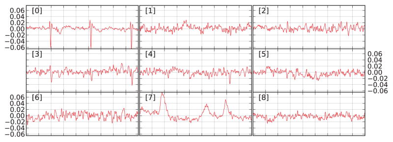
Trellis plot of 9 ICA components. The sources 0 to 5 are reorderd by bivariate Pearson correlation with the ECG channel. The first time series (index 0) displayed in the upper-left window clearly resembles a cardiac signal. The time series 7 closely matches the EOG signal.

MNE handles ICA in a similar manner as an SSP operator; The ICA decomposition can be stored in a FIF file to be accessed later. The unmixing matrix and the selection of the independent sources can then be reviewed and updated as required without having to modify or duplicate the original data. Once the matrices are available, applying them to the data is about as fast as applying SSP projectors.

3.1.5. Combining SSP and ICA

Although SSP and ICA both address the same family of problems, they can be combined in useful ways. The orthonormal basis, as used in SSP, may give a plausible model of environmental noise, but not necessarily so of highly skewed physiological artifact components for which ICA is expected to achieve more accurate signal–artifact separation. On the other hand, the ICA model does not have an explicit noise term. Non-biological artifacts may not be that reliably modeled or detected using ICA, either due to their noise-like distribution, or for not meeting the stationarity requirement in ICA. In practice, it is therefore recommended to first apply empty-room SSP projections and then treat physiological artifacts using ICA. Using MNE-Python covariance objects, optionally equipped with SSP vectors, ICA can take such projections into account when modeling, transforming, and inverse-transforming data.

3.2. Forward modeling

3.2.1. Computation of the magnetic field and and the electric potential

The physical relationship between cerebral electric currents and the extracranial magnetic fields and scalp surface potentials measured by MEG and EEG is governed by Maxwell’s equations. Importantly, the frequencies of the neural electrical signals are sufficiently low to warrant the use of the quasi-static approximation, i.e., the time-dependent terms in Maxwell’s equations can be omitted (Plonsey, 1969; Hämäläinen et al., 1993). Therefore, the MEG/EEG forward problem amounts to providing an accurate enough solution of the quasi-static version of Maxwell’s equations. The problem is further simplified by the fact that we can assume that the magnetic permeability of the head is that of the free space and, therefore, only need to consider the distribution of electrical conductivity.

To solve the forward problem, one needs an approximation of the distribution of the electrical and magnetic properties of the head, the specifications of the elementary source model and the source space, the locations of the EEG electrodes on the scalp and the configurations of the MEG sensors. The elementary source model in MNE is the current dipole, and the electrical conductivity is assumed to be piecewise constant. With the latter approximation we can employ the boundary element model (BEM), see, e.g., (Mosher et al., 1999). MNE supports single- and three-compartment BEMs; the latter has to be employed when EEG data are present (Hämäläinen and Sarvas, 1989). The three compartments need to be nested and correspond to the scalp, the skull, and the brain (cf. Fig. 5). MNE implements the BEM using the linear collocation method (Mosher et al., 1999) with the isolated skull approach (Hämäläinen and Sarvas, 1989) to improve numerical precision. Alternative BEM formulations exist (Mosher et al., 1999; Kybic et al., 2005; Gramfort et al., 2010; Stenroos and Sarvas, 2012) but are not presently implemented in MNE. The default electrical conductivities used by MNE are 0.3 S/m for the brain and the scalp, and 0.006 S/m for the skull, i.e., the conductivity of the skull is assumed to be 1/50 of that of the brain and the scalp.

Figure 5.

Triangulated nested boundary surfaces used in the MNE BEM forward model: the inner skull, the outer skull, and the scalp. The segmentations are obtained from T1 or Flash MRIs using the FreeSurfer package. By default, MNE employs 5120 triangles (2562 vertices) on each surface.

MNE relies on FreeSurfer for the automatic segmentation of the skull and the scalp surfaces. The segmentation can be done from the same T1 MRI used for the FreeSurfer pipeline, which gives the cortical surface segmentation, but also from flash MR images to improve the fidelity of skull segmentation. The triangulations used by MNE usually have 5120 triangles for each of the three surfaces.

In addition to the BEM layers, the forward solver needs the properties of the sensors. For EEG, one only requires the electrode locations, and thus MNE supports all EEG systems with a compatible file format (BrainVision, EDF, eximia). For MEG, the locations, orientations and pick-up loop geometries are needed for all sensors. All major MEG vendors (Neuromag, CTF, 4D, KIT) are supported; the different MEG sensors (magnetometers, axial and planar gradiometers) are implemented with help of a “coil definition” file, which contains the information about the individual pick-up coil geometries. Specifically, the output of the kth MEG sensor, b_k, is approximated by the weighted sum

$$b_{ks}=\sum _{p=1}^{N_k}{w}_{kp}\overrightarrow{B}({\overrightarrow{r}}_{kp};{\overrightarrow{r}}_s,{\widehat{e}}_s)·{\widehat{n}}_{kp}$$ (1)

where B⃗(⇉; ⇉_s, ⇉_s) is the magnetic field at ⇉, generated by a unit current dipole at ⇉_s pointing to direction ê, w_kp are scalar weights, ⇉_kp are locations within the pick-up coil loops comprising the MEG sensor, and ň_kp are the corresponding unit vectors normal to the plane of the pick-up loop. This equation states that the output of an MEG sensor is proportional to the sum of the magnetic fluxes threading the sensing coil loops of the flux transformer of a sensor. The integration over the coil loops is performed numerically rather than analytically using the integration points {⇉_kp, ň_kp} and weights w_kp. The winding direction of the loops is taken into account in w_kp.

The coil definition file contains the numerical integration data for all supported sensor types. Three different accuracies of integration are provided: “minimal”, which usually ignores the finite size of the coil loops, “normal”, which provides sufficient accuracy for practical purposes, and “accurate”, which is the best available accuracy. In addition to the primary sensors on the helmet, the compensation, or reference, magnetometers and gradiometers present in the CTF, 4D, and KIT systems are included in the forward model as well. If the data file to be processed indicates that “virtual gradiometers” have been created using the reference sensors, the forward calculation applies an automatic correction for this noise rejection scheme.

3.2.2. The source space

When working with distributed source models (see Section 3.3) the locations of the elementary dipolar sources need to be specified a priori to compute the forward operator, also known as the gain matrix. This ensemble of dipole locations is called the source space. MNE can handle both volumetric and surface source spaces. For a volumetric source space one must specify the grid spacing, e.g., 5 or 7 mm between neighboring points in 3D space, whereas for a surface-based source space one must specify the surface and the subsampling scheme. In this latter case, MNE by default uses the surface between the gray and the white matter, although this can be changed, e.g. by using a FreeSurfer “mid” surface that is equidistant from white/grey matter interface and pial surface. Subsampling could be done by decimating the surface mesh but preserving surface topology as well as spacing and neighborhood information between vertices can be difficult. Therfore, MNE uses a repeatedly subdivided icosahedron or octahedron as the subsampling method. Once a subdivision step has been accomplished, the resulting polyhedron is overlaid on the cortical surface inflated to a sphere and the cortical vertices closest to the vertices of the the polyhedron are included to the source space. For example, an icosahedron subdivided 5 times, abbreviated ico-5, consists of 10242 locations per hemisphere, which leads to an average spacing of 3.1 mm between dipoles (assuming a surface area of 1000 cm² per hemisphere). Such a source space is presented in Fig. 6. As there is no actual surface decimation, the cortical orientation used for orientation-constrained models is obtained by taking the normal of the high-resolution surface at the selected vertices. In addition, MNE also offers the option to perform a numerical averaging of the normals over a small patch around each selected vertex.

Figure 6.

Cortical segmentation used for the source space in the distributed model with MNE. Left: The pial (red) and white matter (green) surfaces overlaid on an MRI slice. Right: The right-hemisphere part of the source space (yellow dots), represented on the inflated surface of the right hemisphere, was obtained by subdivision of an icosahedron leading to 10242 locations per hemisphere with an average nearest-neighbor distance of 3.1 mm.

3.2.3. Coordinate system alignment

The forward solver requires that the boundary-element surfaces, the source space, and the sensor locations are defined in a common coordinate system. This is made possible by the co-registration step, which outputs the rigid-body transformation (translation and rotation) that relates the MRI coordinate system employed in FreeSurfer and the MEG “head” coordinate system, defined by the fiducial landmarks (two pre-auricular points and the nasion). In the beginning of each MEG study, the locations of the fiducial landmarks, the head-position indicator (HPI) coils, EEG electrodes, and a cloud of scalp surface points are digitized and the MEG head coordinate system is set up. The position of the MEG sensor array in the MEG head coordinates is determined in the beginning (and end) of each recording by feeding currents to the HPI coils and using the MEG sensor array to measure the resulting magnetic fields. In addition, some systems offer the possibility for recording the head position continuously during the actual acquisition and compensation methods to bring all the data to a common coordinate frame, see, e.g., (Uutela et al., 2001; Taulu et al., 2005).

As a result of acquiring the digitization and head position data and possibly applying post-measurement correction for head movements, all information required for MEG–MRI co-registration is available in the FIF files. An initial estimate for the coordinate transformation is obtained by manually identifying the fiducial landmarks from the MRI-based rendering of the head surface. This initial approximation is then automatically refined by using the iterative closest-point algorithm (Besl and McKay, 1992) which optimizes the transformation given the requirement that the digitized scalp surface points must be as close as possible to the MRI-defined scalp. The accuracy of this step is particularly crucial for precise source estimation (Hillebrand and Barnes, 2003). The co-registration tools are available both in MNE-C and MNE-Python.

3.2.4. Summary

As described above, the solution of the forward problem involves a number of steps with a few parameters that have well-established default values. The forward computation pipeline in MNE is fully automatic thanks to the underlying FreeSurfer software. The only manual step is the co-registration, which takes a couple of minutes and needs to be done only once for each MEG session.

3.3. Inverse modeling

Although careful sensor-level data analysis can offer important insight into the location and timing of neural activity, the accurate localization of the underlying neural sources is of major interest for neuroscientific research. For this purpose, the MNE software implements several methods for solving the electromagnetic inverse problem using distributed source spaces, either surface-based or volumetric. MNE employs the same noise-covariance matrix to whiten the data and the forward solution consistently in all implemented source estimation methods.

For reconstructing the source current density, the MNE software implements the minimum norm estimate (MNE), i.e., the Bayesian maximum a posteriori (MAP) estimate with a Gaussian prior distribution on the source amplitudes (Hämäläinen and Ilmoniemi, 1984; Dale and Sereno, 1993; Hämäläinen and Ilmoniemi, 1994). In order to account for the depth localization bias known for MNE, that is, the tendency of MNE methods to favor superficial sources, the MNE software allows to apply a depth-weighting scheme based on scaling the source covariance matrix (Fuchs et al., 1999; Lin et al., 2006b). This approach is often referred to as the weighted minimum norm estimate (wMNE).

The MNE solution can be computed without restricting the source orientations. However, following the general assumption that the primary sources of MEG and EEG signals are postsynaptic currents in the apical dendrites of cortical pyramidal neurons, the net current can be assumed to be normal to the cortical mantle. MNE can constrain the dipole orientations when a cortical surface source space is employed.

The first option is to fix the source orientations to be normal to the underlying surface, which can either be computed based on a single source or on the statistics of a cortical surface patch surrounding the source location. This is known as a fixed-orientation solution (Dale and Sereno, 1993). Accordingly, there is an option in MNE software to compute the forward solution for dipoles oriented normal to the cortical mantle only. However, it is recommended to always compute the gain matrix for all dipole orientations because the depth weighting parameter for wMNE cannot be set correctly without this information (Lin et al., 2006b). Alternatively, the fixed orientation constraint can be relaxed (Lin et al., 2006a). In this loose orientation constraint approach, the variances of the source components oriented tangentially to the cortical surface are scaled by 0 < β < 1, where β = 0 is equivalent to the fixed orientation constraint and β = 1 corresponds to free dipole orientations. The parameter β can also be set automatically and be made location-dependent by using the cortical patch statistics, i.e., the variance of the cortical normals within the patch corresponding to each source space point (Lin et al., 2006a) to determine β for each cortical source site.

In addition to reconstructing the actual current density, the MNE software includes two methods for computing noise-normalized linear inverse estimates. These methods, namely dynamic statistical parameter mapping (dSPM) (Dale et al., 2000) and standardized low-resolution brain electromagnetic tomography (sLORETA) (Pascual-Marqui, 2002), transform the current density values into dimensionless statistical quantities, which help identify where the estimated current differs significantly from baseline noise. Moreover, the noise-normalized methods reduce the location bias of the estimates. In particular, the tendency of the MNE to prefer superficial currents is reduced, and the width of the point-spread function becomes more uniform across the cortex (Dale et al., 2000). An example of a dSPM source estimate is shown in Fig. 7.

Figure 7.

Source localization of an auditory N100 component using dSPM. The regularization parameter was set to correspond to SNR = 3 in the whitened data, source orientation had a loose constraint (β = 0.2), and depth weighting was set to 0.8 (all three default values).

In order to include a priori information on the source location coming from other measurement modalities, the MNE software allows to compute fMRI-guided linear inverse estimates (Dale et al., 2000). The fMRI weighting involves two steps. First, the fMRI activation map is thresholded at a user-defined value to identify significant fMRI activations. Thereafter, the elements of the source-covariance matrix corresponding to sources being located in regions falling below the threshold are scaled down by a user-defined factor (Liu et al., 1998). It is important to note that the fMRI weighting has a strong influence on the MNE solution, whereas the noise-normalized estimates are less affected.

As an addition to the linear inverse methods, the MNE software also includes estimation of equivalent current dipoles (ECDs). At present, dipole fitting is limited to a single ECD at a single time point. The fitting procedure is based on a four-step approach. First, an initial guess of the ECD location is determined by an exhaustive search through a predefined grid. Thereafter, a Nelder-Mead simplex optimization is applied and the risk of arriving at a local minimum is reduced by repeating the optimization using the result of the first minimization as an initial guess; the best solution (highest goodness-of-fit) is retained. Finally, the ECD amplitude is computed.

All methods mentioned above can be applied as batch-mode commands or by using the interactive mne_analyze tool, a graphical user interface provided by the MNE-C code that can also be used for the visual inspection of the source reconstruction results. Alternatively, snapshots and movies of the source reconstruction results can be saved for inspection and processing with a batch-mode command. Python also offers brain visualization capabilities through the PySurfer package (http://pysurfer.github.com). Both MNE-C and MNE-Python allow the user to display source maps in a customizable fashion. MNE-Python extends some of these capabilities by making it much easier to automate generation and annotation of figures via scripting of graphical calls.

In addition to the inverse methods mentioned above, the MNE-Python package contains a set of imaging methods based on spatio–temporal sparse priors, which allow reconstruction of spatially sparse, i.e., ECD-like source estimates with a distributed source model. These priors are applied either in the time domain, e.g., the minimum current estimate (MCE) (Matsuura and Okabe, 1995; Uutela et al., 1999), the γ-MAP estimate detailed in (Wipf and Nagarajan, 2009), and the mixed norm estimate (MxNE) (Ou et al., 2009; Gramfort et al., 2012), or in the time–frequency domain, e.g., the time–frequency mixed norm estimate (TF-MxNE) (Gramfort et al., 2013) (Fig. 8). Furthermore, an implementation of the linearly constrained minimum variance (LCMV) beamformer (Veen et al., 1997) in the time domain is part of the repertoire of MNE-Python, see Fig. 9.

Figure 8.

Source localization obtained with the time–frequency mixed-norm estimates (TF-MxNE) (Gramfort et al., 2013) for the right visual condition. The labels of the primary and secondary visual cortices (V1 in red and V2 in yellow) estimated by FreeSurfer from the T1 MRI are overlaid on the cortical surface.

Figure 9.

Source localization with LCMV Beamformer. A volumetric grid source space was used with the left temporal MEG channels to localize the origin of the N100 component in the left auditory cortex.

3.4. Surface-based normalization

While clinical examinations generally consider data from a single patient, neuroscience questions are often answered by comparing and combining data from a group of subjects. To achieve this, data from all participating subjects need to be transformed to a common space. This procedure is called spatial normalization in the fMRI literature. MNE software exploits the FreeSurfer spherical coordinate system defined for each hemisphere (Dale et al., 1999; Fischl et al., 1999) to accomplish such normalization. For data defined on a subsampled version of the cortical tesselation (including source estimates), morphing from one brain to another comprises three steps. First, to associate all vertices of the high-resolution cortical tesselation with data, the estimates are spread to neighboring vertices using an isotropic diffusion process parametrized by the number of iterations. Second, the FreeSurfer registration is used to linearly interpolate data defined on the subject’s brain to the average brain; this interpolation is encapsulated in morph maps. Finally, the data defined on the average brain is subsampled to yield the same number of source locations in all subjects. The procedure is illustrated in Fig. 10 using dSPM estimates of the auditory N100m response.

Figure 10.

Current estimates obtained in an individual subject can be remapped (morphed), i.e., normalized, to another cortical surface, such as that of the FreeSurfer average brain “fsaverage” shown here. The normalization is done separably for both hemispheres using a non-linear registration procedure defined on the sphere (Dale et al., 1999; Fischl et al., 1999). Here, the N100m auditory evoked response is localized using dSPM and then mapped to “fsaverage”.

3.5. Frequency and time–frequency representations

For several types of M/EEG data analysis it is relevant to quantify oscillatory activity as a function of time and location (Buzsaki, 2006). This is achieved by computing frequency or time–frequency representations of the data. It is worth noting that “oscillations” usually refers to the existence of narrow-band signals whereas in neuroscience literature this term is used more liberally and refers to division of the data to several frequency bands, each of which may have a substantial width. Depending on the bandwidth and signal characteristics, the data may thus resemble band-limited noise rather than oscillations at few distinct frequencies.

Frequency and time–frequency representations include estimation of the power spectra of empty-room M/EEG data for quality control and to find sources of interference, the estimation of induced power in the sensor and source spaces, and connectivity estimation. The MNE-Python package provides functions to compute frequency representations, time–frequency representations, and power spectra in sensor and source space.

The most fundamental non-parametric frequency-domain representation of the data is the power spectrum. It can be estimated using the discrete Fourier transform (DFT), which can be computed efficiently using fast Fourier transform (FFT) algorithms (Cooley and Tukey, 1965). Important parameters in frequency domain transforms are the sampling rate, the number of samples to use, and the resulting frequency resolution. These factors are directly related: if the data were acquired with a sampling rate of f_s and N real-valued time samples are input to the DFT, the resulting complex-valued spectrum (representing amplitude and phase) will consist of N/2 equispaced frequency samples from 0 to f_s/2 − f_s/N (this assumes that N is even; the spacing is slightly different when N is odd). Note that the upper bound is the Nyqvist frequency f_s/2, which is the highest frequency that can be faithfully represented when sampling a continuous signal at a rate of f_s. While the lowest frequency of the spectral estimate is 0, it is important to realize that the data segment has to be sufficiently long to allow reliable estimation of the low-frequency end of the spectrum. As a rule of thumb, the length of the data segment should correspond to at least 5 periods (cycles) of the signal at the lowest frequency of interest. For example, if one is interested in the spectrum around 1 Hz, it is recommended to use data segments at least 5 s long (e.g., for wavelet analysis see Lin et al. (2004a); Ghuman et al. (2011)).

A problem that is also related to the finite length of the data segment is spectral leakage; a purely sinusoidal signal will yield a spectrum with one main lobe at the frequency of the sinusoid and several side lobes. This effect can be mitigated by multiplying the data segment with a windowing function in the time domain. A Hann window (often called “Hanning window”) is typically used in MNE software, which gives a good trade-off between the width of the main lobe and suppression of side lobes. In MNE software, power spectra of raw data are estimated by averaging the magnitudes of DFTs of data segments with a length and overlap specified by the user. This procedure is known as Welch’s method for spectral estimation (Welch, 1967). The resulting source-space power spectrum can be exported as a file for visualization using mne_analyze or it can be analyzed further.

While the averaging employed in Welch’s method reduces the variance of the estimate and proper windowing reduces spectral leakage, more accurate spectra can be obtained using the multi-taper method for spectral estimation (Thomson, 1982). This method also uses DFT but it employs a set of orthogonal windowing functions, known as Slepian tapers or discrete prolate spheroidal sequences (DPSS), and then computes a weighted average of the obtained spectra. By using adaptive weights for each frequency, the multi-taper method can further reduce spectral leakage, which is particularly useful for signals with a large dynamic range. Compared to Welch’s method, the multi-taper method obtains a more accurate spectrum at the price of an increased computational cost. In MNE, we provide multi-taper functions for the estimation of power spectra in sensor and source space.

Pure frequency representations assume stationarity, i.e., that the spectrum does not change over time. For M/EEG data this assumption often does not hold. For example, in event-related experiments, the spectral composition of the signals evolves rapidly during the response to the stimulus. For such data, it is more meaningful to compute a time–frequency representation, which can show the changing spectrum over time. In MNE, time–frequency representations are obtained using Morlet wavelets, which are constructed by multiplying complex sinusoids (90-deg phase difference between the real and imaginary parts) at frequencies of interest with Gaussian windows (Morlet et al. (1982); for a MEG application, see Lin et al. (2004b); Tallon-Baudry and Bertrand (1999)). The user can adjust the transformation by specifying the frequencies of interest and the number of cycles in the wavelets at each frequency; a higher number of cycles results in wider Gaussian windows and thus better frequency resolution but poorer temporal resolution.

We provide functions to compute time–frequency representations in both sensor and source space. Fig. 11 shows an example of an induced power change, i.e., averaged power computed over an ensemble of epochs as opposed to evoked power obtained from averaged epochs, in response to electric stimulation of the left median nerve at wrist. This analysis demonstrates a strong stimulus-induced power increase at about 20 Hz and starting about 500 ms after the stimulus. Such rebounds of the oscillatory activity in the somatomotor system are well known induced responses (Hari and Salmelin, 1997).

Figure 11.

Induced power change in the hand region along the right central sulcus. A total of 111 epochs were used for the computation. The data in each epoch were transformed to the source space using the dSPM method. The time–frequency representation was obtained using 23 Morlet wavelets with center frequencies 8–30 Hz. The number of cycles used increased linearly with the frequency; 4 cycles were used for 8 Hz and 15 cycles for 30 Hz. Finally, the obtained time–frequency representation was averaged over a region of interest in the source space, a.k.a. “label”, in the right central sulcus. The power was baseline-corrected to display percentage of variation (“3” means a 3-fold increase in power compared to the pre-stimulus baseline).

When computing source-space power spectra or time–frequency representations with linear inverse operators (MNE, dSPM, sLORETA), MNE exploits the linearity of the operations to improve efficiency as there are typically far more source points than sensors. This is accomplished by computing the DFT in sensor space, applying the inverse operator on the complex-valued result and taking the magnitude at the source level.

3.6. Connectivity estimation

MNE can compute several bivariate connectivity measures in both the sensor and source space. The supported measures are all spectral, i.e., they are based on estimates of cross spectral densities and, depending on the measure, power spectral densities. Currently, the connectivity module in MNE can compute coherence, coherency (complex-valued coherence), imaginary coherence (Nolte et al., 2004), phase-locking value (PLV) (Lachaux et al., 1999), pairwise phase consistency (PPC) (Vinck et al., 2010), which is an unbiased estimate of PLV, phase lag index (PLI) (Stam et al., 2007), and weighted phase lag index (WPLI) (Vinck et al., 2011). In addition, the unbiased squared PLI and de-biased squared WPLI can be estimated (Vinck et al., 2011). Some methods, like imaginary coherence and WPLI, down weight zero-lag interactions and are therefore less affected by spurious interactions that exist in M/EEG sensor and source space data due to finite spatial resolution (Schoffelen and Gross, 2009). The use of the unbiased and de-biased versions of the estimators is recommended when connectivity is estimated based on a small number of epochs. We refer to the above references for further details of each measure. The connectivity can be computed either in the frequency or time–frequency domain using the appropriate transforms described in the previous section.

To compute reliable connectivity estimates, the spectral estimation has to be performed using tens or even hundreds of observations. In MNE, the observations are obtained by dividing the raw data into epochs using event timings. For data that does not have events associated with them, e.g., recordings of spontaneous brain activity, functions are provided to generate events at fixed intervals, which enables connectivity computation for such data. To compute sensor-space connectivity, the epochs can be directly passed to the connectivity estimation routine. By default, the connectivity measures between all N sensor time series are computed, which, due to symmetry, results in N(N − 1)/2 connectivity estimates for all included frequency or time– frequency bins. For some experiments, one may only be interested in the connectivity between selected pairs of time series, e.g., between a seed and all other time series. In MNE, the user can specify for which pairs of time series the connectivity estimation should be performed.

The ability to compute the connectivity estimates for a subset of connections is especially useful when connectivity is estimated in the source space, where the number of time series is much larger than in the sensor space and all-to-all connectivity computation can be prohibitive. In order to estimate source-space connectivity, the epoch data are first projected to source space by means of one of the inverse methods described earlier. Typically, either MNE, dSPM, sLORETA, or LCMV should be used as these methods work well for single-epoch estimates where the SNR is low. Moreover, these linear methods are computationally efficient. It is important to note that spectral estimates are meaningful only when the source estimates are signed. Therefore, when performing the inverse computation, the current component oriented perpendicular to the cortical mantle must be used instead of combining the components for the three spatial dimensions, which would result in unsigned (magnitude) estimates. The obtained source estimates, one for each epoch, are then passed to the connectivity estimation routine.

As noted before, the large number of source-space time series makes all-to-all connectivity estimation computationally very demanding. An attractive option is therefore to reduce the number of time series and thus the computational demand by summarizing the source time series within a set of cortical regions. We provide functions to do this automatically for cortical parcellations obtained by FreeSurfer, which employs probabilistic atlases and cortical folding patterns for an automated subject-specific segmentation of the cortex into anatomical regions (Fischl et al., 2004; Desikan et al., 2006; Destrieux et al., 2010). The obtained set of summary time series can then be used as input to the connectivity estimation. The association of time series with cortical regions simplifies the interpretation of results and it makes them directly comparable across subjects since, due to the subject-specific parcellation, each time series corresponds to the same anatomical region in each subject. A result of such an analysis is illustrated in Fig. 12, where the connectivity was computed for 68 cortical regions in the FreeSurfer “aparc” parcellation.

Figure 12.

Visualization of connectivity resulting from the presentations of a visual flash to the left visual hemifield. The connectivity was computed for –200– –500 ms relative to the stimulus onset over 67 epochs. The inverse was computed using the dSPM method, with a source-space resolution of 8196 vertices (oct-6). The source estimates were summarized into 68 time series corresponding to the regions in the FreeSurfer “aparc” parcellation. All-to-all connectivity was computed in the alpha band (8– –13 Hz) using the de-biased squared WPLI method (Vinck et al., 2011) with multi-taper spectral estimation. Finally, the connectivity was visualized as a circular graph using a connectivity visualization routine provided in MNE-Python.

Due to the potentially large number of time series and epochs used for connectivity computation, an efficient implementation is important. In MNE, we reduce the computational cost by giving the user the option to compute several connectivity measures at once, which reduces the computational demand as the spectral estimation only has to be performed once. Furthermore, parallel processing enabled by modern multi-core processors can be used to greatly reduce the computation time.

Memory limitations are also important to consider. Assuming an oct-6 source-space resolution (8196 vertices), 512 frequency points, and double-precision floating point representation, storing the multi-taper spectral estimate with 7 tapers for a single epoch requires 224 MB of memory. Therefore, a simplistic implementation which first computes the spectral estimates leads to excessive memory requirements when the connectivity is computed over hundreds or even thousands of epochs. In MNE, we avoid this problem by using pipelined processing which is entirely hidden from the user; the user can write a linear script which first extracts epochs, computes the inverse for each epoch, and then passes the result to the connectivity estimation function. However, internally, the actual computation is delayed in the sense that during the connectivity estimation, single epochs are extracted from the raw file, the inverse is applied, and the spectra are estimated. However, for linear inverses, higher computational efficiency is again achieved by automatically applying the time–frequency or wavelet transforms in sensor space before applying the inverse to the transformed data, which (due to linearity of the operations) results in the source-space spectral estimates. This implementation leads to computationally efficient connectivity estimation with memory requirements that are independent of the number of epochs, which makes it possible to estimate source-space connectivity on desktop computers and laptops with only a few GB of memory.

3.7. Statistics

The non-parametric statistical tests (Maris and Oostenveld, 2007) implemented in MNE are designed to provide a generic framework for statistical analysis. This framework has been designed to be flexible enough for the user to configure the clustering structure to reflect the underlying topological features of interest. For example, the algorithms can be used to cluster in time, which operates based on temporal adjacency alone, or in the time–frequency space, which operates by examining temporally and spectrally contiguous regions. Both of these approaches would be appropriate for dipole fits or region-of-interest activations. Alternatively, clustering can be performed spatio-temporally, where the spatial adjacency of sensors or dipole locations in source space would be taken into account to identify spatially and temporally contiguous regions of significant activity. Since this clustering procedure is independent of the statistic employed to determine similarity between the observations defining clusters, another important implication of the non-parametric cluster-statistics approach is that arbitrary statistical functions can be used in combination with arbitrary contrasts. Currently, MNE-Python directly supports one-sample t-tests, two-sample t-tests, one-way F-tests and two-way repeated-measures ANOVA for clustering-permutation tests. Additional statistical functions are provided by other scientific and numerical Python packages, but also user-defined functions can be included with ease as demonstrated in the MNE documentation.

Once significant clusters are obtained, functions are provided to help summarize them. The temporal center of mass is obtained by weighting each time point by the number of significant vertices, while the spatial center of mass is obtained by weighting each vertex by the number of significant time points. The spatial center of mass can then be easily transformed into MNI Talairach coordinates for simple comparison to previous neuroimaging studies (Larson and Lee, 2012).

4. Discussion

Data processing, such as M/EEG analysis, can be thought of as a chain or pipeline of operations, where each step has an impact on the results. In the preceding sections we have discussed particular choices made in the MNE software to proceed from preprocessing to advanced applications such as statistics in source space, including surface based registration for group studies, or connectivity measures between brain regions of interest.

MNE provides a few modules with graphical user interfaces (GUIs) that are valuable in inspecting and exploration of the data. However, we suggest that all of the processing should be done with scripts in which all parameters can be defined. The software has been designed with this concept in mind. Data visualization GUIs are provided in Python for every stage of processing (raw data, epoched data, evoked data, SSP effects, time–frequency analysis, source estimates, cluster inspection, etc.), but provide very limited functionality for anything besides inspecting the data. The idea is that the GUIs should allow users to be comfortable with (and understand) the effects of the chosen parameters, such as the baseline interval, regularization of MNE/dSPM/sLORETA inversion, or the amount of smoothing used for morphing the source time courses. The downside of this approach is that MNE users are expected to have basic programming skills to write shell, Matlab, or Python scripts. However, given the number of code snippets and examples available on the MNE web site, a user typically ends up copy-pasting blocks of code to assemble their own pipeline. This choice can still limit the user base and the impact of the software, however, this approach has clear benefits. First, our experience from analyzing several M/EEG studies indicates that the processing pipeline needs to be tailored for each study. Even though most pipelines follow the same logic including filtering, epoching, averaging, etc., the number of options is large even for such standard steps. Scripting gives the flexibility to set those options and handle the requirements of different M/EEG studies.

Second, an analysis conducted with the help of scripts leads to more reproducible results. Indeed, reproducing a statistic or a figure can be done by re-executing a script with the same input data. Scripting is also a way to prevent errors that users might introduce by inadvertently changing their behavior in the middle of the analysis, or because they are running multiple studies simultaneously and for data from one subject they use the parameters of another study. As the procedures and steps chosen are accurately recorded in a script, the script is an efficient way to communicate one’s research strategy to colleagues, who in return may provide more concise feedback targeting the level of program code in addition to parameter descriptions from a report. This ultimately helps identify bugs and errors, thereby improving the quality of the particular research project. Nevertheless, it should be pointed out that analysis steps requiring user interaction, e.g., time-varying dipole fits, which are presently not incorporated in MNE, can also be made highly reproducible by proper training and scrutiny (Stenbacka et al., 2002).

Finally, studies that involve processing of data from dozens or hundreds of subjects are made tractable via scripting. This is particularly relevant in an era of large-scale data analysis where massive cohorts of subjects may number more than a thousand, cf., the Human Brain Project or the Human Connectome Project (Van Essen et al., 2012).

Today neuroscientists from different academic disciplines spend an increasing amount of time writing software to process their experimental data. Data analysis is not limited to neuroimaging; Nowadays almost all scientific data are processed by computers and software programs. The practical consequence of this, is that the correctness of the science produced relies on the quality of the software written (Dubois, 2005). The success of digital data analysis is made possible by high-quality data, by sophisticated numerical and mathematical methods, and last but not least by correct implementations. The MNE software, in particular the MNE-Python project, is developed and maintained to work toward high quality in terms of accuracy, efficiency and readability of the code. In order to measure and establish accuracy, the development process requires writing of unit and regression tests to ensure the installation of the software is correct and that the results it gives match with results previously obtained across multiple different computing platforms. This testing framework currently covers about 88% of the MNE-Python code. Besides allowing users to track the stability and accuracy of the software, this also makes it easier to incorporate new contributions quickly without inadvertently breaking existing code.

By leveraging this open development approach, MNE has received many contributions from the community. To control their quality, the policy in MNE development is that any code contribution must be read by two or more people, the author and one reviewer at minimum. This practice aims at establishing coding conventions that facilitate code readability and bug fixing by users as has been demonstrated in other projects (Marchenko et al., 2009; Bhat and Nagappan, 2006; George and Williams, 2004). Importantly, the entire source code (including the full development history) is made publicly available by a distributed version control system. This makes it straightforward to keep track of the project’s development and thus handle code changes in a way that minimizes the risk of rendering existing scripts and analysis pipelines inoperable. Finally, large parts of the source code are commented using inline documentation that allows for automatically building user manuals in PDF and HTML formats. The Ohloh.net¹¹ source code analysis project attests that 36% of the source code consists of documentation and with this, MNE-Python’s extent of documentation scores in the upper third of the Python projects publicly trackable. See (Aruliah et al., 2012; Prlić and Procter, 2012) for a more detailed presentation of the best practices for scientific software development beyond the field of neuroimaging.

The MNE community employs a mailing list (mne analysis@nmr.mgh.harvard.edu; requires an approval to subscribe and post) as the primary support channel, but also makes use of online services such as Twitter to announce new features and bug fixes, and Github to report bugs and propose new features. Github is then used to follow the progress made on bug fixes and added features.

As advocated above, scientific results should be easily reproducible. In addition, applying existing analysis methods on new data should be straighforward as that fosters new scientific discoveries. In other words, analysis pipelines should be reusable across laboratories. Towards that end, the MNE software package and Brainstorm have converged on many aspects of the standard analysis pipeline, such as the implementation of various noise-normalization methods. Continued sharing of methods and best practices facilitates research reproducibility.

In order to maximize the impact of software, care must be taken about the license governing its use. The MNE-Python and MNE-Matlab code are for this reason provided under the very permissive Open Source BSD license. This license allows anybody to reuse and redistribute this code, even for commercial applications. The MNE-Matlab code is for example redistributed with Brainstorm (Tadel et al., 2011), FieldTrip (Oostenveld et al., 2011), NutMeg (Dalal et al., 2011) and SPM (Litvak et al., 2011) to read and write FIF files.

Neuroimaging is a broad field encompassing static images, such as anatomical MRI as well as dynamic, functional data such M/EEG or fMRI. The MNE software relies on other packages such as FreeSurfer for anatomical MRI processing, or NiBabel (http://nipy.org/nibabel) for reading and writing images such as standard NIfTI files. Our ambition is not to make MNE self-contained; the MNE package cannot and does not aim to do everything. MNE has its own scope and leverages the capabilities of external software in the neuroimaging software ecosystem. Tighter integration with fMRI analysis pipelines could be facilitated by NiPype (Gorgolewski et al., 2011) but is first made possible by adopting standards. That is why all data MNE produces are stored in FIF file format which can be read and written by various software packages. The MNE-Python code also relies on core scientific libraries, namely Numpy and Scipy (Milmann and Avaizis, 2011), and works with standard datastructures (Van der Walt et al., 2011) that are also used in most scientific Python packages.

Good science requires not only good hypothesis and theories, creative experimental designs, and principled analysis methods, but also well-established data analysis tools and software. A scientific discovery is the end of a long chain, which will break at its weakest link. The MNE software provides a solid foundation for reproducible scientific discoveries based M/EEG data. As the contributions to the MNE software package continue to grow, the MNE software suite should provide increasing value to the neuroimaging community that has not only helped determine its current form, but continues to shape its future.

Highlights.

• The MNE software provides a complete pipeline for MEG and EEG data analysis

• MNE covers preprocessing, forward modeling, inverse methods, and visualization

• MNE supports advanced analysis: time-frequency, statistics, and connectivity

• MNE-Python enables fast and memory-efficent processing of large data sets

• The MNE-Python is open-source software supporting a collaborative development effort

References

- Aine C, Sanfratello L, Ranken D, Best E, MacArthur J, Wallace T, Gilliam K, Donahue C, Montao R, Bryant J, Scott A, Stephen J. Meg-sim: A web portal for testing meg analysis methods using realistic simulated and empirical data. Neuroinformatics. 2012;10:141–158. doi: 10.1007/s12021-011-9132-z. [DOI] [PMC free article] [PubMed] [Google Scholar]
- Aruliah DA, Brown CT, Hong NPC, Davis M, Guy RT, Haddock SHD, Huff K, Mitchell I, Plumbley M, Waugh B, White EP, Wilson G, Wilson P. Best practices for scientific computing. CoRR. 2012 doi: 10.1371/journal.pbio.1001745. abs/1210.0530. [DOI] [PMC free article] [PubMed] [Google Scholar]
- Barnett L, Seth AK. Behaviour of granger causality under filtering: Theoretical invariance and practical application. Journal of Neuroscience Methods. 2011;201 (2):404– 419. doi: 10.1016/j.jneumeth.2011.08.010. URL http://www.sciencedirect.com/science/article/pii/S0165027011004687. [DOI] [PubMed] [Google Scholar]
- Becker RA, Cleveland WS, Shyu M-J, Kaluzny SP, et al. A tour of Trellis graphics. AT & T Bell Laboratories; 1996. [Google Scholar]
- Besl P, McKay ND. A method for registration of 3-d shapes. Pattern Analysis and Machine Intelligence, IEEE Transactions on. 1992;14 (2):239–256. [Google Scholar]
- Bhat T, Nagappan N. Evaluating the efficacy of test-driven development: industrial case studies. Proceedings of the 2006 ACM/IEEE international symposium on Empirical software engineering; ACM. 2006. pp. 356–363. [Google Scholar]
- Brookes M, Woolrich M, Luckhoo H, Price D, Hale J, Stephenson M, Barnes G, Smith S, Morris P. Investigating the electrophysiological basis of resting state networks using magnetoencephalography. Proceedings of the National Academy of Sciences of the United States of America. 2011;108 (40):16783–16788. doi: 10.1073/pnas.1112685108. [DOI] [PMC free article] [PubMed] [Google Scholar]
- Buzsaki G. Rhythms of the Brain. 1. Oxford University Press; USA: Aug, 2006. [Google Scholar]
- Cooley JW, Tukey JW. An algorithm for the machine calculation of complex fourier series. Mathematics of computation. 1965:297–301. [Google Scholar]
- Dalal SS, Zumer JM, Guggisberg AG, Trumpis M, Wong DDE, Sekihara K, Nagarajan SS. Meg/eeg source reconstruction, statistical evaluation, and visualization with nutmeg. Computational Intelligence and Neuroscience. 2011 doi: 10.1155/2011/758973. [DOI] [PMC free article] [PubMed] [Google Scholar]
- Dale A, Fischl B, Sereno M. Cortical surface-based analysis i: Segmentation and surface reconstruction. NeuroImage. 1999;9:179–194. doi: 10.1006/nimg.1998.0395. [DOI] [PubMed] [Google Scholar]
- Dale A, Liu A, Fischl B, Buckner R. Dynamic statistical parametric mapping: combining fMRI and MEG for high-resolution imaging of cortical activity. Neuron. 2000;26:55–67. doi: 10.1016/s0896-6273(00)81138-1. [DOI] [PubMed] [Google Scholar]
- Dale A, Sereno M. Improved localization of cortical activity by combining EEG and MEG with MRI cortical surface reconstruction: a linear approach. Journal of Cognitive Neuroscience. 1993;5 (2):162–176. doi: 10.1162/jocn.1993.5.2.162. [DOI] [PubMed] [Google Scholar]
- Delorme A, Makeig S. Eeglab: an open source toolbox for analysis of single-trial eeg dynamics including independent component analysis. Journal of Neuroscience Methods. 2004;134:9–21. doi: 10.1016/j.jneumeth.2003.10.009. [DOI] [PubMed] [Google Scholar]
- Delorme A, Mullen T, Kothe C, Acar ZA, Bigdely-Shamlo N, Vankov A, Makeig S. Eeglab, sift, nft, bcilab, and erica: new tools for advanced eeg processing. Intell. Neuroscience 2011. 2011 Jan;10:10–10. 10. doi: 10.1155/2011/130714. URL http://dx.doi.org/10.1155/2011/130714. [DOI] [PMC free article] [PubMed] [Google Scholar]
- Desikan RS, Ségonne F, Fischl B, Quinn BT, Dickerson BC, Blacker D, Buckner RL, Dale AM, Maguire RP, Hyman BT, Albert M, Killiany R. An automated labeling system for subdividing the human cerebral cortex on mri scans into gyral based regions of interest. NeuroImage. 2006;31 (3):968–980. doi: 10.1016/j.neuroimage.2006.01.021. [DOI] [PubMed] [Google Scholar]
- Destrieux C, Fischl B, Dale A, Halgren E. Automatic parcellation of human cortical gyri and sulci using standard anatomical nomenclature. NeuroImage. 2010;53 (1):1. doi: 10.1016/j.neuroimage.2010.06.010. [DOI] [PMC free article] [PubMed] [Google Scholar]
- Dubois P. Maintaining correctness in scientific programs. Computing in Science and Engineering. 2005 May;7 (3):80–85. [Google Scholar]
- Fischl B, Sereno M, Dale A. Cortical surface-based analysis ii: Inflation, flattening, and a surface-based coordinate system. NeuroImage. 1999;9:195–207. doi: 10.1006/nimg.1998.0396. [DOI] [PubMed] [Google Scholar]
- Fischl B, Van Der Kouwe A, Destrieux C, Halgren E, Ségonne F, Salat DH, Busa E, Seidman LJ, Goldstein J, Kennedy D, Caviness V, Makris N, Rosen B, Dale A. Automatically parcellating the human cerebral cortex. Cerebral Cortex. 2004;14 (1):11–22. doi: 10.1093/cercor/bhg087. [DOI] [PubMed] [Google Scholar]
- Florin E, Gross J, Pfeifer J, Fink GR, Timmermann L. The effect of filtering on granger causality based multivariate causality measures. NeuroImage. 2010;50 (2):577– 588. doi: 10.1016/j.neuroimage.2009.12.050. URL http://www.sciencedirect.com/science/article/pii/S1053811909013391. [DOI] [PubMed] [Google Scholar]
- Fries P. Neuronal gamma-band synchronization as a fundamental process in cortical computation. Annual review of neuroscience. 2009;32:209–224. doi: 10.1146/annurev.neuro.051508.135603. [DOI] [PubMed] [Google Scholar]
- Friston KJ. Functional and effective connectivity in neuroimaging: a synthesis. Human Brain Mapping. 1994;2 (1–2):56–78. [Google Scholar]
- Fuchs M, Wagner M, Kohler T, Wischmann HA. Linear and nonlinear current density reconstructions. J Clin Neurophysiol. 1999;16 (3):267–295. doi: 10.1097/00004691-199905000-00006. 99353451 0736-0258 Journal Article Review Review, Tutorial. [DOI] [PubMed] [Google Scholar]
- George B, Williams L. A structured experiment of test-driven development. Information and software Technology. 2004;46 (5):337–342. [Google Scholar]
- Ghuman AS, McDaniel JR, Martin A. A wavelet-based method for measuring the oscillatory dynamics of resting-state functional connectivity in MEG. Neuroimage. 2011 Jan; doi: 10.1016/j.neuroimage.2011.01.046. [DOI] [PMC free article] [PubMed] [Google Scholar]
- Gorgolewski K, Burns CD, Madison C, Clark D, Halchenko YO, Waskom ML, Ghosh SS. Nipype: a flexible, lightweight and extensible neuroimaging data processing framework in python. Front Neuroinform. 2011 Aug;5(13) doi: 10.3389/fninf.2011.00013. [DOI] [PMC free article] [PubMed] [Google Scholar]
- Gramfort A, Kowalski M, Hämäläinen M. Mixed-norm estimates for the m/eeg inverse problem using accelerated gradient methods. Physics in Medicine and Biology. 2012 Mar;57 (7):1937–1961. doi: 10.1088/0031-9155/57/7/1937. [DOI] [PMC free article] [PubMed] [Google Scholar]
- Gramfort A, Papadopoulo T, Olivi E, Clerc M. OpenMEEG: opensource software for quasistatic bioelectromagnetics. BioMed Eng OnLine. 2010;9 (1):45. doi: 10.1186/1475-925X-9-45. [DOI] [PMC free article] [PubMed] [Google Scholar]
- Gramfort A, Strohmeier D, Haueisen J, Hmlinen M, Kowalski M. Time-frequency mixed-norm estimates: Sparse m/eeg imaging with non-stationary source activations. NeuroImage. 2013;70 (0):410– 422. doi: 10.1016/j.neuroimage.2012.12.051. [DOI] [PMC free article] [PubMed] [Google Scholar]
- Granger C. Investigating causal relations by econometric models and cross-spectral methods. Econometrica: Journal of the Econometric Society. 1969;37 (3):424–438. [Google Scholar]
- Granger C, Hatanaka M. Spectral analysis of economic time series. Princeton Univ. Press; 1964. [Google Scholar]
- Gross J, Baillet S, Barnes G, Henson R, Hillebrand A, Jensen O, Jerbi K, Litvak V, Maess B, Oostenveld R, Parkkonen L, Taylor J, van Wassenhove V, Wibral M, Schoffelen J. Good practice for conducting and reporting meg research. NeuroImage. 2013 Jan;65 (15):349–363. doi: 10.1016/j.neuroimage.2012.10.001. [DOI] [PMC free article] [PubMed] [Google Scholar]
- Gross J, Kujala J, Hämäläinen M, Timmermann L. Dynamic imaging of coherent sources: studying neural interactions in the human brain. Proceedings of the National Academy of Sciences. 2001 Jan;98 (2):694–699. doi: 10.1073/pnas.98.2.694. [DOI] [PMC free article] [PubMed] [Google Scholar]
- Hämäläinen M, Hari R, Ilmoniemi R, Knuutila J, Lounasmaa O. Magnetoencephalography - Theory, instrumentation, and applications to noninvasive studies of the working human brain. Reviews of modern physics. 1993;65 (2):413–497. [Google Scholar]
- Hämäläinen M, Ilmoniemi R. Tech Rep TKK-F-A559. Helsinki University of Technology; 1984. Interpreting magnetic fields of the brain: minimum norm estimates. [DOI] [PubMed] [Google Scholar]
- Hämäläinen M, Ilmoniemi R. Interpreting magnetic fields of the brain: minimum norm estimates. Med Biol Eng Comput. 1994 Jan;32 (1):35–42. doi: 10.1007/BF02512476. [DOI] [PubMed] [Google Scholar]
- Hämäläinen MS, Sarvas J. Realistic conductivity geometry model of the human head for interpretation of neuromagnetic data. IEEE Transactions on Biomedical Engineering. 1989 Feb;36 (2):165–171. doi: 10.1109/10.16463. [DOI] [PubMed] [Google Scholar]
- Hari R. On brain’s magnetic responses to sensory stimuli. Journal of clinical neurophysiology : official publication of the American Electroencephalographic Society. 1991 Apr;8 (2):157–169. doi: 10.1097/00004691-199104000-00004. [DOI] [PubMed] [Google Scholar]
- Hari R, Salmelin R. Human cortical oscillations: a neuromagnetic view through the skull. Trends Neurosci. 1997 Jan;20 (1):44–49. doi: 10.1016/S0166-2236(96)10065-5. [DOI] [PubMed] [Google Scholar]
- Haufe S, Nikulin VV, Müller KR, Nolte G. A critical assessment of connectivity measures for EEG data: A simulation study. NeuroImage. 2012;64:120–133. doi: 10.1016/j.neuroimage.2012.09.036. [DOI] [PubMed] [Google Scholar]
- Hillebrand A, Barnes GR. The use of anatomical constraints with MEG beamformers. NeuroImage. 2003 Dec;20 (4):2302–2313. doi: 10.1016/j.neuroimage.2003.07.031. [DOI] [PubMed] [Google Scholar]
- Hipp JF, Hawellek DJ, Corbetta M, Siegel M, Engel AK. Large-scale cortical correlation structure of spontaneous oscillatory activity. Nature neuroscience. 2012 Jun;15 (6):884–890. doi: 10.1038/nn.3101. [DOI] [PMC free article] [PubMed] [Google Scholar]
- Hyvärinen A, Oja E. Independent component analysis: algorithms and applications. Neural networks. 2000 doi: 10.1016/s0893-6080(00)00026-5. [DOI] [PubMed] [Google Scholar]
- Jung TP, Makeig S, Humphries C, Lee TW, Mckeown MJ, Iragui V, Sejnowski TJ. Removing electroencephalographic artifacts by blind source separation. Psychophysiology. 2000;37:163–178. [PubMed] [Google Scholar]
- Khan S, Gramfort A, Shetty NR, Kitzbichler MG, Ganesan S, Moran JM, Lee SM, Gabrieli JD, Tager- Flusberg HB, Joseph RM, et al. Local and long-range functional connectivity is reduced in concert in autism spectrum disorders. Proceedings of the National Academy of Sciences. 2013;110 (8):3107–3112. doi: 10.1073/pnas.1214533110. [DOI] [PMC free article] [PubMed] [Google Scholar]
- Kybic J, Clerc M, Abboud T, Faugeras O, Keriven R, Papadopoulo T. A common formalism for the integral formulations of the forward EEG problem. IEEE Transactions on Medical Imaging. 2005;24 (1):12–28. doi: 10.1109/tmi.2004.837363. [DOI] [PubMed] [Google Scholar]
- Lachaux JP, Rodriguez E, Martinerie J, Varela FJ, et al. Measuring phase synchrony in brain signals. Human Brain Mapping. 1999;8 (4):194–208. doi: 10.1002/(SICI)1097-0193(1999)8:4<194::AID-HBM4>3.0.CO;2-C. [DOI] [PMC free article] [PubMed] [Google Scholar]
- Larson E, Lee AKC. The cortical dynamics underlying effective switching of auditory spatial attention. NeuroImage. 2012 Sep; doi: 10.1016/j.neuroimage.2012.09.006. [DOI] [PMC free article] [PubMed] [Google Scholar]
- Lin F, Belliveau J, Dale A, Hämäläinen M. Distributed current estimates using cortical orientation constraints. Hum Brain Mapp. 2006a;27:1–13. doi: 10.1002/hbm.20155. [DOI] [PMC free article] [PubMed] [Google Scholar]
- Lin FH, Witzel T, Ahlfors SP, Stufflebeam SM, Belliveau JW, Hamalainen MS. Assessing and improving the spatial accuracy in meg source localization by depth-weighted minimum-norm estimates. Neuroimage. 2006b;31 (1):160–71. 1053–8119. doi: 10.1016/j.neuroimage.2005.11.054. (Print) Journal Article. [DOI] [PubMed] [Google Scholar]
- Lin FH, Witzel T, Hmlinen MS, Dale AM, Belliveau JW, Stufflebeam SM. Spectral spatiotemporal imaging of cortical oscillations and interactions in the human brain. Neuroimage. 2004a Sep;23 (2):582–595. doi: 10.1016/j.neuroimage.2004.04.027. [DOI] [PMC free article] [PubMed] [Google Scholar]
- Lin FH, Witzel T, Hamalainen MS, Dale AM, Belliveau JW, Stufflebeam SM. Spectral spatiotemporal imaging of cortical oscillations and interactions in the human brain. Neuroimage. 2004b;23 (2):582–95. 1053–8119. doi: 10.1016/j.neuroimage.2004.04.027. (Print) Journal Article. [DOI] [PMC free article] [PubMed] [Google Scholar]
- Litvak V, Mattout J, Kiebel S, Phillips C, Henson R, Kilner J, Barnes G, Oostenveld R, Daunizeau J, Flandin G, Penny W, Friston K. Eeg and meg data analysis in spm8. Computational Intelligence and Neuroscience. 2011;2011 doi: 10.1155/2011/852961. [DOI] [PMC free article] [PubMed] [Google Scholar]
- Liu AK, Belliveau JW, Dale AM. Spatiotemporal imaging of human brain activity using functional mri constrained magnetoencephalography data: Monte carlo simulations. Proc Natl Acad Sci U S A. 1998;95 (15):8945–50. doi: 10.1073/pnas.95.15.8945. [DOI] [PMC free article] [PubMed] [Google Scholar]
- Marchenko A, Abrahamsson P, Ihme T. Agile Processes in Software Engineering and Extreme Programming. Springer; 2009. Long-term effects of test-driven development a case study; pp. 13–22. [Google Scholar]
- Maris E, Oostenveld R. Nonparametric statistical testing of EEG- and MEG-data. J Neurosci Methods. 2007 Aug;164 (1):177–90. doi: 10.1016/j.jneumeth.2007.03.024. [DOI] [PubMed] [Google Scholar]
- Martinsson P-G, Rokhlin V, Tygert M. A randomized algorithm for the decomposition of matrices. Applied and Computational Harmonic Analysis 2010 Feb; [Google Scholar]
- Matsuura K, Okabe Y. Selective minimum-norm solution of the biomagnetic inverse problem. IEEE Transactions on Biomedical Engineering. 1995 Jun;42 (6):608–615. doi: 10.1109/10.387200. [DOI] [PubMed] [Google Scholar]
- Milmann K, Avaizis M, editors. Scientific Python. Vol. 11 of Computing in Science & Engineering. IEEE/AIP; Mar, 2011. [Google Scholar]
- Mitra P, Bokil H. Observed Brain Dynamics. Oxford University Press; New York: 2008. [Google Scholar]
- Morlet J, Arens G, Fourgeau E, Giard D. Wave Propagation and Sampling Theory : Part I : Complex signal and scattering multilayered - Part II : Sampling Theory and complex waves. Geophysics. 1982;47:203–236. [Google Scholar]
- Mosher J, Baillet S, Leahy R. Equivalence of linear approaches in bioelectromagnetic inverse solutions. 2003 IEEE Workshop on Statistical Signal Processing; Oct, 2003. pp. 294–297. [Google Scholar]
- Mosher J, Leahy R. RecursiveMUSIC: A framework for EEG andMEG source localization. Biomedical Engineering, IEEE Transactions on. 1998 Jan; doi: 10.1109/10.725331. [DOI] [PubMed] [Google Scholar]
- Mosher JC, Leahy RM, Lewis PS. Eeg and meg: forward solutions for inverse methods. IEEE Trans Biomed Eng. 1999;46 (3):245–59. 0018–9294. doi: 10.1109/10.748978. (Print) Journal Article. [DOI] [PubMed] [Google Scholar]
- Nichols TE, Holmes AP. Nonparametric permutation tests for functional neuroimaging: a primer with examples. Human Brain Mapping. 2002 Jan;15 (1):1–25. doi: 10.1002/hbm.1058. [DOI] [PMC free article] [PubMed] [Google Scholar]
- Nolte G, Bai O, Wheaton L, Mari Z, Vorbach S, Hallett M. Identifying true brain interaction from eeg data using the imaginary part of coherency. Clinical Neurophysiology. 2004;115 (10):2292–2307. doi: 10.1016/j.clinph.2004.04.029. [DOI] [PubMed] [Google Scholar]
- Oostenveld R, Fries P, Maris E, Schoffelen J-M. Open source software for advanced analysis of meg, eeg, and invasive electrophysiological data. Computational Intelligence and Neuroscience. 2011;2011 doi: 10.1155/2011/156869. [DOI] [PMC free article] [PubMed] [Google Scholar]
- Ou W, Hämaläinen M, Golland P. A distributed spatio-temporal EEG/MEG inverse solver. NeuroImage. 2009 Feb;44 (3):932–946. doi: 10.1016/j.neuroimage.2008.05.063. [DOI] [PMC free article] [PubMed] [Google Scholar]
- Pantazis D, Nichols TE, Baillet S, Leahy RM. A comparison of random field theory and permutation methods for the statistical analysis of MEG data. NeuroImage. 2005 Mar;25 (2):383–394. doi: 10.1016/j.neuroimage.2004.09.040. [DOI] [PubMed] [Google Scholar]
- Pascual-Marqui R. Standardized low resolution brain electromagnetic tomography (sLORETA): technical details. Methods Find Exp Clin Pharmacology. 2002;24 (D):5–12. [PubMed] [Google Scholar]
- Pedregosa F, Varoquaux G, Gramfort A, Michel V, Thirion B, Grisel O, Blondel M, Prettenhofer P, Weiss R, Dubourg V, Vanderplas J, Passos A, Cournapeau D, Brucher M, Perrot M, Duchesnay E. Scikit-learn: Machine learning in Python. Journal of Machine Learning Research. 2011;12:2825–2830. [Google Scholar]
- Pérez F, Granger BE. IPython: a System for Interactive Scientific Computing. Comput Sci Eng. 2007 May;9(3):21–29. URL http://ipython.org. [Google Scholar]
- Plonsey R. Bioelectric phenomena. McGraw-Hill; New York: 1969. [Google Scholar]
- Prlić A, Procter JB. Ten simple rules for the open development of scientific software. PLoS Comput Biol. 2012;8(12) doi: 10.1371/journal.pcbi.1002802. [DOI] [PMC free article] [PubMed] [Google Scholar]
- Ridgway GR, Litvak V, Flandin G, Friston KJ, Penny WD. The problem of low variance voxels in statistical parametric mapping; a new hat avoids a “haircut”. NeuroImage. 2012 Feb;59 (3):2131–2141. doi: 10.1016/j.neuroimage.2011.10.027. [DOI] [PMC free article] [PubMed] [Google Scholar]
- Robinson S, Vrba J. Functional neuroimaging by synthetic aperture magnetometry. In: Yoshimoto T, Kotani M, Kuriki S, Karibe H, Nakasato N, editors. Recent Advances in Biomagnetism. Tohoku University Press; Sendai, Japan: 1998. pp. 302–305. [Google Scholar]
- Schelter B, Winterhalder M, Timmer J. Wiley com. 2006. Handbook of Time Series Analysis. [Google Scholar]
- Scherg M, Von Cramon D. Two bilateral sources of the late AEP as identified by a spatio-temporal dipole model. Electroencephalogr Clin Neurophysiol. 1985 Jan;62 (1):32–44. doi: 10.1016/0168-5597(85)90033-4. [DOI] [PubMed] [Google Scholar]
- Schoffelen JM, Gross J. Source connectivity analysis with MEG and EEG. Human brain mapping. 2009 Jun;30 (6):1857–1865. doi: 10.1002/hbm.20745. [DOI] [PMC free article] [PubMed] [Google Scholar]
- Sorrentino A, Parkkonen L, Pascarella A, Campi C, Piana M. Dynamical MEG source modeling with multi-target bayesian filtering. Hum Brain Mapp. 2009;30 (6):1911–1921. doi: 10.1002/hbm.20786. URL http://www.ncbi.nlm.nih.gov/pubmed/19378276. [DOI] [PMC free article] [PubMed] [Google Scholar]
- Stam CJ, Nolte G, Daffertshofer A. Phase lag index: assessment of functional connectivity from multi channel eeg and meg with diminished bias from common sources. Human Brain Mapping. 2007;28 (11):1178–1193. doi: 10.1002/hbm.20346. [DOI] [PMC free article] [PubMed] [Google Scholar]
- Stenbacka L, Vanni S, Uutela K, Hari R. Comparison of minimum current estimate and dipole modeling in the analysis of simulated activity in the human visual cortices. Neuroimage. 2002;16 (4):936–43. doi: 10.1006/nimg.2002.1151. [DOI] [PubMed] [Google Scholar]
- Stenroos M, Sarvas J. Bioelectromagnetic forward problem: isolated source approach revis(it)ed. Phys Med Biol. 2012;57 (11):3517–35. doi: 10.1088/0031-9155/57/11/3517. [DOI] [PubMed] [Google Scholar]
- Tadel F, Baillet S, Mosher JC, Pantazis D, Leahy RM. Brainstorm: A user-friendly application for meg/eeg analysis. Computational Intelligence and Neuroscience. 2011;2011 doi: 10.1155/2011/879716. [DOI] [PMC free article] [PubMed] [Google Scholar]
- Tallon-Baudry C, Bertrand O. Oscillatory gamma activity in humans and its role in object representation. Trends Cogn Sci. 1999;3 (4):151–162. 1364–6613. doi: 10.1016/s1364-6613(99)01299-1. Journal article. [DOI] [PubMed] [Google Scholar]
- Tallon-Baudry C, Bertrand O, Wienbruch C, Ross B, Pantev C. Combined eeg and meg recordings of visual 40 hz responses to illusory triangles in human. Neuroreport NA. 1997;(5):1103–7. doi: 10.1097/00001756-199703240-00008. [DOI] [PubMed] [Google Scholar]
- Taulu S. Spatiotemporal Signal Space Separation method for rejecting nearby interference in MEG measurements. Physics in Medicine and Biology. 2006;51 (7):1759–1769. doi: 10.1088/0031-9155/51/7/008. [DOI] [PubMed] [Google Scholar]
- Taulu S, Simola J, Kajola M. Applications of the signal space separation method. IEEE Trans Signal Proc. 2005;53(9):3359–3372. [Google Scholar]
- Thomson DJ. Spectrum estimation and harmonic analysis. Proceedings of the IEEE. 1982;70 (9):1055–1096. [Google Scholar]
- Uusitalo M, Ilmoniemi R. Signal-space projection method for separating meg or eeg into components. Medical and Biological Engineering and Computing. 1997;35 (2):135–140. doi: 10.1007/BF02534144. [DOI] [PubMed] [Google Scholar]
- Uutela K, Hämäläinen M, Somersalo E. Visualization of magnetoencephalographic data using minimum current estimates. NeuroImage. 1999;10:173–180. doi: 10.1006/nimg.1999.0454. [DOI] [PubMed] [Google Scholar]
- Uutela K, Taulu S, Hamalainen M. Detecting and correcting for head movements in neuromagnetic measurements. Neuroimage. 2001;14 (6):1424–1431. doi: 10.1006/nimg.2001.0915. [DOI] [PubMed] [Google Scholar]
- Van der Walt S, Colbert S, Varoquaux G. The NumPy array: a structure for efficient numerical computation. Computing in Science and Engineering. 2011:11. [Google Scholar]
- Van Essen D, Ugurbil K, Auerbach E, Barch D, Behrens T, Bucholz R, Chang A, Chen L, Corbetta M, Curtiss S, Della Penna S, Feinberg D, Glasser M, Harel N, Heath A, Larson-Prior L, Marcus D, Michalareas G, Moeller S, Oostenveld R, Petersen S, Prior F, Schlaggar B, Smith S, Snyder A, Xu J, Yacoub E. The human connectome project: A data acquisition perspective. NeuroImage. 2012 Oct;62 (4):2222–2231. doi: 10.1016/j.neuroimage.2012.02.018. [DOI] [PMC free article] [PubMed] [Google Scholar]
- Veen BV, Drongelen WV, Yuchtman M, Suzuki A. Localization of brain electrical activity via linearly constrained minimum variance spatial filtering. Biomedical Engineering, IEEE Transactions on. 1997 Jan;44 (9):867–880. doi: 10.1109/10.623056. [DOI] [PubMed] [Google Scholar]
- Vinck M, Oostenveld R, van Wingerden M, Battaglia F, Pennartz C. An improved index of phase-synchronization for electrophysiological data in the presence of volume-conduction, noise and sample-size bias. NeuroImage. 2011;55 (4):1548–1565. doi: 10.1016/j.neuroimage.2011.01.055. [DOI] [PubMed] [Google Scholar]
- Vinck M, van Wingerden M, Womelsdorf T, Fries P, Pennartz C. The pairwise phase consistency: a bias-free measure of rhythmic neuronal synchronization. NeuroImage. 2010;51 (1):112–122. doi: 10.1016/j.neuroimage.2010.01.073. [DOI] [PubMed] [Google Scholar]
- Wang JZ, Williamson SJ, Kaufman L. Magnetic source images determined by a lead-field analysis: the unique minimum-norm least-squares estimation. IEEE Transactions on Biomedical Engineering. 1992 Jul;39 (7):665–675. doi: 10.1109/10.142641. [DOI] [PubMed] [Google Scholar]
- Welch P. The use of fast fourier transform for the estimation of power spectra: a method based on time averaging over short, modified periodograms. IEEE Transactions on Audio and Electroacoustics. 1967;15 (2):70–73. [Google Scholar]
- Wiener N. Modern mathematics for engineers. McGraw-Hill; New York: 1956. The theory of prediction. [Google Scholar]
- Wipf D, Nagarajan S. Beamforming using the relevance vector machine. Proceedings of the 24th international conference on Machine learning. ICML ‘07; New York, NY, USA: ACM; 2007. pp. 1023–1030. URL http://doi.acm.org/10.1145/1273496.1273625. [Google Scholar]
- Wipf D, Nagarajan S. A unified Bayesian framework for MEG/EEG source imaging. NeuroImage. 2009 Feb;44 (3):947–966. doi: 10.1016/j.neuroimage.2008.02.059. [DOI] [PMC free article] [PubMed] [Google Scholar]
- Wolters CH, Köstler H, Möller C, Härdtlein J, Grasedyck L, Hackbusch W. Numerical mathematics of the subtraction method for the modeling of a current dipole in eeg source reconstruction using finite element head models. SIAM J Scientific Computing. 2007;30 (1):24–45. [Google Scholar]