The geometry of Niggli reduction: BGAOL –embedding Niggli reduction and analysis of boundaries

An implicit embedding of the space of Niggli-reduced cells in a higher-dimensional space to facilitate calculation of distances between cells is described. This distance metric is used to create a program, BGAOL, for Bravais lattice determination. Results from BGAOL are compared with results from other metric based Bravais lattice determination algorithms. This embedding depends on understanding the boundary polytopes of the Niggli-reduced cone N in the six-dimensional space G ⁶.

Abstract

Niggli reduction can be viewed as a series of operations in a six-dimensional space derived from the metric tensor. An implicit embedding of the space of Niggli-reduced cells in a higher-dimensional space to facilitate calculation of distances between cells is described. This distance metric is used to create a program, BGAOL, for Bravais lattice determination. Results from BGAOL are compared with results from other metric based Bravais lattice determination algorithms. This embedding depends on understanding the boundary polytopes of the Niggli-reduced cone N in the six-dimensional space G ₆. This article describes an investigation of the boundary polytopes of the Niggli-reduced cone N in the six-dimensional space G ⁶ by algebraic analysis and organized random probing of regions near one-, two-, three-, four-, five-, six-, seven- and eightfold boundary polytope intersections. The discussion of valid boundary polytopes is limited to those avoiding the mathematically interesting but crystallographically impossible cases of zero-length cell edges. Combinations of boundary polytopes without a valid intersection in the closure of the Niggli cone or with an intersection that would force a cell edge to zero or without neighboring probe points are eliminated. In all, 216 boundary polytopes are found. There are 15 five-dimensional boundary polytopes of the full G ⁶ Niggli cone N.

1. Introduction  

In a quantitative science, usable metrics should be defined. In the study of crystal lattices, only a few metrics have been proposed for describing the distance between two lattices (i.e. unit cells). The V7 metric (Andrews et al., 1980 ▶) is quite nonlinear and has known issues in many cases. The metric of Oishi-Tomiyasu (2012 ▶) is nonlinear and changes algorithm in some regions. This study and the work of Macíček & Yordanov (1992 ▶) use a metric based on the differences in metric tensors. This metric is nonlinear outside the Niggli cone. Here we propose a process for obtaining a linear measure from the differences of metric tensors by remaining inside the Niggli cone.

BGAOL (Bravais general analysis of lattices) is a Bravais lattice identification program based on the analysis of Niggli reduction described below. Niggli reduction defines a complex space that has not previously been fully analyzed. Several authors have published interesting commentaries on the properties of this complex space (Hosoya, 2000 ▶; Oishi-Tomiyasu, 2012 ▶; Gruber, 1997 ▶). These studies use the space (Andrews & Bernstein, 1988 ▶), or a similar metric tensor-based space, or a projection of to a space of lower dimensionality, respectively.

Failure to correctly identify the Bravais lattice of a crystal can compromise subsequent least-squares calculations or even the solution of a structure. There are two commonly used ways to obtain a unique representative of the infinite number of cells that may be used to generate a given lattice: Niggli reduction (Niggli, 1928 ▶) and Delaunay reduction (Delaunay, 1932 ▶). We follow the conventions of International Tables for Crystallography (Burzlaff et al., 1992 ▶) in basing this article on Niggli reduction, and we will recast the discussion in terms of Delaunay reduction in a future study.

Given a precisely determined reduced cell, the lattice symmetry may be unambiguously inferred. In addition, reduced cells are useful in searching for sub- and super-cells, in indexing of powder patterns, and in twinned crystal studies. Without a suitable metric and a clear understanding of the geometry of the boundaries of the space, either searches of lattices in the neighborhood of a given cell must be excessively broad and produce many false positives, or, if made tighter, they risk missing important candidates, especially in the vicinity of 90° angles.

As noted by Azaroff & Buerger (1958 ▶), the concept of a reduced cell is strongly related to the concept of a reduced ternary quadratic form (Seeber, 1831 ▶; Selling, 1874 ▶). Reduced cells have become an important computational tool in crystallography (just as reduced quadratic forms are an important tool in computational number theory), but much of the literature focuses on an essentially qualitative approach, taking a reduced cell as an absolute indicator of symmetry and not considering the impact of experimental error (Andrews & Bernstein, 1988 ▶). Consideration of experimental error requires the use of a distance metric dealing with reduced cells. Such metrics have been used in a six-dimensional approach (Zim­mermann & Burzlaff, 1985 ▶), another six-dimensional approach (Andrews & Bernstein, 1988 ▶), a similar six-dimensional approach with a modified norm (Oishi-Tomiyasu, 2012 ▶), a lattice-specific six-dimen­sional approach (Kabsch, 2013 ▶), a B-matrix approach (Macíček & Yordanov, 1992 ▶) and a ‘distortion index’ approach (Minor & Otwinowski, 1997 ▶).

In addition, because the processes of both Niggli and Delaunay reduction can produce large discontinuities in reduced cell parameters from small changes in the lattice, an effective use of a metric must allow for such discontinuities, either by a combinatorial search or by a metric preserving embedding in a higher-dimensional space that removes the discontinuities. Until now, crystallographic software appears either to have used a demanding combinatorial approach or simply to have given up on doing a complete search. The purpose of this article is to take the necessary first steps towards adding an embedding to the existing combinatorial approaches by clearly mapping the boundary discontinuities and their related transformations.

Two principal uses of Niggli reduction are the determination of Bravais lattice type and the construction of a database using a representation of the unit cell for its key (Andrews et al., 1980 ▶; Toby, 1994 ▶; Byram et al., 1996 ▶).

Both uses can be viewed as distance determinations in . In the former case the distances to the Bravais lattice subspaces are used, and in the latter case the distances between pairs of unit cells are used. However, the complexity of the space has consequences in some regions; it is not adequate to consider only one representation of a unit cell in . A standard mathematical solution is to create an ‘embedding’ (Nash, 1956 ▶) of the space with an appropriate associated metric. In such an embedding, separate regions of the space under consideration are sewn together into a single fundamental region preserving distances from the original piecewise presentation.

In the case being considered the regions contain sets of cells that appear to be far apart originally but which can be seen to represent similar lattices as the regions are sewn together, and sets of cells that remain far apart after the sewing can be seen as not representing similar lattices. In concept, this is similar to what we do in folding of atomic coordinates into the asymmetric unit of a crystal. This is an example of a simple embedding, allowing us to see which atoms interact. This is the approach followed in BGAOL. The present article discusses the application to Bravais lattice identification. McGill et al. (2014 ▶) discuss the database application.

In order to define an embedding, the operations defining the fundamental region must be specified. In the case of Niggli reduction, the complete space is , and the fundamental region is the fraction of the space containing only Niggli-reduced cells. Proper unit cells in any other region of can be transformed into the fundamental region by the rules of Niggli reduction. The transformations at the boundaries must be enumerated and their combinations analyzed as in Appendix A (see Table 1 ▶).

Table 1. Fifteen five-dimensional boundary polytopes of Niggli-reduced cells in .

For a given boundary polytope , the column ‘Condition’ gives the constraints (prior to closure) of the boundary polytope. Boundary polytopes 1 and 2 apply in both the all-acute () and the all-obtuse () branches of the Niggli-reduced cone. Boundary polytopes 8, B, E and F are restricted to the all-obtuse () branch of the Niggli-reduced cone, . Boundary polytopes 6, 7, 9, A, C and D are restricted to the all-acute () branch of . Boundary polytopes 3, 4 and 5 are boundaries of both the all-acute () and the all-obtuse () branches.

Class	Boundary	Condition	Transformation matrix
Equal cell edges	1
	2
90°	3
	4
	5
Face diagonal	6	and
	7	and
	8
	9	and
	A	and
	B
	C	and
	D	and
	E
Body diagonal	F

Given the complete set of conditions that define all boundaries of the fundamental unit and their relationships to adjacent units, the transformations of coordinates on crossing the boundaries are enumerated. Oishi-Tomiyasu (2012 ▶) has enumerated transformations in a related space.

There have been multiple investigations of such boundaries, albeit without a consideration of experimental error in most cases. See, for example, Gruber (1997 ▶, 2006 ▶) for a review and an approach using a five-dimensional space based on the metric tensor. Gruber’s 1997 ▶ approach partitions the space of reduced cells into 127 disjoint components (genera), based on 67 one- to four-dimensional ‘hyperfaces’ further subdivided into 227 hyperfaces in order to achieve a common partitioning applicable to both Niggli and Delaunay reduction. Unfortunately, Gruber’s reduction to five dimensions, and any purely topological approach without a metric that allows error propagation from the experimental data, makes it difficult or impossible to carry out a full perturbation analysis of the impact of experimental errors. The linear metric used in the embedding makes such error analysis simpler.

Therefore, in this investigation we return to the full six-dimensional space (Andrews & Bernstein, 1988 ▶), , of unit cells based on the metric tensor and use algebraic techniques confirmed by a Monte Carlo technique to explore the ‘natural’ five-, four-, three-, two- and one-dimensional boundary polytopes of the six-dimensional polytope of Niggli-reduced cells. The two techniques are mutually supportive. The lower-dimensional boundaries are an algebraic consequence of the five-dimensional boundaries. The lower-dimensional boundaries derived algebraically are confirmed by the Monte Carlo technique, which helps to identify unpopulated boundaries and boundaries that drop to lower dimension owing to glancing intersections with multiple other boundaries.

There are 15 five-dimensional boundary polytopes and a total of 216 boundary polytopes. In this approach, all the boundary polytopes are on the surface of the closure of the six-dimensional Niggli-reduced polytope. Identification of these boundary polytopes and the reduction transformations to be applied in crossing them is an essential step either in a combinatorial error analysis or in embedding into a higher-dimensional space for an analytical error analysis, and it is useful for database searches.

The 15 five-dimensional boundary polytopes give the complete shape of the space of Niggli-reduced cells (see Appendix A ). All of the primitive lattice types can be represented as combinations of the 15 five-dimensional boundary polytopes. All of the non-primitive lattice types can be represented as combinations of the 15 five-dimensional boundary polytopes and of the seven special-position subspaces of the five-dimensional boundary polytopes. By confining our attention to just the Niggli reduction, the result is a simpler classification than Gruber’s with more direct applicability to an embedding and database searching.

2. Background  

Crystallography began with the study of crystal morphology and the classification of substances by the shapes of their crystals, a database concept before the creation of databases. Von Laue (1952 ▶) provided an accessible description. Two themes have developed: Bravais lattice assignment and database searches to identify substances by their unit-cell parameters. In this article we consider only the Bravais lattice identification issues.

The following glossary may be helpful in reading the subsequent discussion.

(1) . The six-dimensional space of vectors

See § A1.

(2) N, Niggli cone, Niggli-reduced polytope. The locus of points in G ⁶ that are Niggli reduced. See § A2.

(3) Negative or positive portions of the Niggli cone. Those parts of the Niggli cone that have either all negative or all positive. Together they constitute the entire Niggli cone.

(4) Manifold. A space that in local regions has mappings that establish Euclidean coordinates.

(5) Polytope. A portion of a space with flat sides.

(6) Boundary of a set. The points that have some immediate neighbors in the set and some immediate neighbors not in the set, i.e. the interface between the inside of the set and the points outside of the set. Boundary points need not themselves be members of the set.

(7) Boundary transformations. The transformations to be applied to a point as it crosses from inside the Niggli cone to outside in order to transform its position to the corresponding position inside the Niggli cone.

(8) Boundary polytope. A portion of the boundary that is a polytope, i.e. has flat sides.

(9) Special-position subspace of a boundary polytope. The locus of points in a boundary manifold that are invariant under the boundary transformation. See § A4.

(10) Embedding (in topology). The mapping of one space into another, often of higher dimensionality.

(11) Isometric embedding. An embedding that preserves distances.

(12) L1 norm. Manhattan or city-block distance, the sum of the magnitudes of the differences of the vector components.

(13) L2 norm. Euclidean distance, the square root of the sum of the squares of the differences of the vector components.

(14) Fundamental region. For a repeating mathematical structure, one is chosen as the starting point. For instance, in crystallography, the 0–1, 0–1, 0–1 unit cell is often chosen as the basic cell.

(15) Bravais lattice subspace. Any polytope in that is occupied by a single Bravais lattice type. For instance, cF lattices fall on a line with base vector (1, 1, 1, 1, 1, 1).

(16) Hyperface. Term used by Gruber (1997 ▶) for subspaces.

(17) Monte Carlo. Mathematical technique of random multiple probing of a system to discover its responses.

(18) Glancing intersection. An intersection of a manifold with the intersection of two or more other manifolds, but of measure zero. For instance, in a plane, the line (−1, 1) has a glancing intersection with the all-plus quadrant.

(19) Boundary maps. The list of transformations that must be applied to points exiting the fundamental unit.

(20) Projector into a subspace. A linear mapping from an arbitrary point in a space to the nearest point in the subspace.

(21) Closure. For an open manifold, the closure is the content of the manifold plus the content of the boundary. For instance, the closure of a circular region is the interior of the circle plus the bounding circle.

2.1. Bravais lattice assignment  

Modern work on Bravais lattice assignment has taken two directions: qualitative absolute assignment of lattice type versus quantitative assignment using a metric to measure the distance from the 14 Bravais lattice types. This is a fuzzy distinction because all methods are fundamentally quantitative, being rooted in numeric cell parameters. The advantage of the methods based on, and making full use of, a metric is that they perform well in the presence of experimental error. The more fine grained the metric used, the more easily and efficiently can the alternatives be ranked. Gruber’s work (Gruber, 1997 ▶) is the latest in qualitative assignment of lattice types. DELOS (Zimmermann & Burzlaff, 1985 ▶) is a popular example of a rather coarse-grained metric. Kabsch has incorporated a fine-grained metric in XDS (Kabsch, 1993 ▶, 2010 ▶) based on the sum of the magnitudes of deviations from the various Niggli reduction conditions. See Macíček & Yordanov (1992 ▶) for a reasonably complete review of the relevant literature.

The use of a fine-grained metric under which it is meaningful to ask precisely how far a probe cell is from a given lattice and to compare that distance with the experimental error began with Andrews & Bernstein (1988 ▶), in which the space , consisting of vectors

(a modified metric tensor), was introduced. The concept is simple, but the implementation is complex because a very large number of iterations may be necessary to apply the boundary transformations of the Niggli cone. BLAF (Macíček & Yordanov, 1992 ▶) and OT-BLD (Oishi-Tomiyasu, 2012 ▶) cut off the iterations, creating the possibility of missed symmetries. The implementation of Andrews & Bernstein (1988 ▶), ITERATE, continues without a cutoff until no new candidates are found, to avoid missed symmetries but at the expense of additional execution time. BGAOL resolves this conflict by specifically using the 15 five-dimensional boundaries cited in Appendix A , labeled 1, 2, 3, 4, 5, 6, 7, 8, 9, A, B, C, D, E, F, from which the many remaining internal boundaries of the Niggli cone may be derived as intersections, and by using an isometric (i.e. distance-preserving) embedding that sharply limits the boundary transforms to be applied to the ones directly involved with those 15 five-dimensional boundaries, plus three of the four-dimensional boundaries (8F, BF and EF) in the negative portion of the Niggli cone and two boundaries (69 and 6C) in the positive portion of the Niggli cone that contains the images of 8F, BF and EF under their boundary transforms. For the database application involving points far from the boundaries, additional four-dimensional boundaries and three-dimensional boundaries are used.

2.2. Embeddings  

In mathematics, an embedding is an instance of some mathematical structure within another, described as a map from one structure to the other. Among the purposes of embedding is to map coordinates from a discontinuous space onto a continuous one. An example would be a computer screen where objects exiting to the right reappear on the left. That can be modeled by mapping the screen onto a cylinder and treating the screen coordinate as an angle with range zero to . Two of the ways that embeddings can be implemented are by analytical embedding, where an equation would map between the spaces, and by a collection of boundary maps with actions at the boundaries specified in the map. Treating the above example as cylinder is an analytical embedding. Using a boundary map that says at the right side subtract the screen width and at the left side add the screen width is a boundary map embedding. The latter are frequently used when an analytical embedding is difficult to determine or simply unknown. Often an analytical embedding is a more understandable, compact description, but boundary maps are frequently the more practical. We implemented our embedding of as boundary maps (there is no known analytical mapping), unfolding some transformations that are isometric across the boundaries (essentially an analytical embedding). This may seem to be an overly complex way to describe the distance measure, but it is useful in this case where the distance measure varies outside the fundamental unit (see §2.3).

The problem of finding how far cells in the Niggli cone are from other cells in the Niggli cone is similar to the problem of finding the distance between atoms in a crystal, where the shortest distance may not be the distance within the asymmetric unit of the chosen cell. For example, in Fig. 1 ▶, two atoms, A and B, are shown in the asymmetric unit of a cell chosen from a two-dimensional lattice, with symmetry-related copies of those atoms in neighboring cells. In this case, a symmetry-related copy of B is closer to A (shown with a solid black line) than is the original B in the same asymmetric unit. An alternative to searching through neighboring cells in two dimensions examining all the translational copies would be to pick up the matching left and right edges of the cell and glue them together to form a tube, and then bend the tube to glue the remaining edges together to form a torus. Then we can navigate between points on the surface of the torus (where there is only one copy of B) looking for the shortest distance. Mapping the torus back onto the flat lattice, the shortest path from A to B consists of the three pieces shown in Fig. 1 ▶ as the bold black segments 1, 2 and 3. Even though they appear to be disjoint in the two-dimensional representation, they are contiguous in the embedding.

Figure 1.

Example of the difficulty of finding the shortest distance in a lattice. The distance within the asymmetric unit of the chosen cell is shown as a light dotted line. However, the shortest distance, shown as a heavy solid line, crosses multiple unit cells.

This process of picking up a lower-dimensional manifold in which we know the geometry in Euclidean patches and gluing the edges of the patches together to form a closed surface in a higher-dimensional space but with the same distances between points is called an isometric embedding. ‘All’ we need to know is the distance function on that embedded surface.

2.3. Metric distortions  

Embedding the Niggli cone in into a higher-dimensional space is, as one might expect, more complicated than embedding a three-dimensional lattice as a torus-like object into a six-dimensional space. In addition to having more dimensions, the symmetry operations generated by the boundary transformations in Table 1 ▶ are not, in general, isometric. The face-diagonal boundary transformations through and the body-diagonal boundary transformation significantly compress space in some directions and expand it in others. In measuring the distance between cells in the Niggli cone, we always have to measure distances between representatives of cells within the Niggli cone and not between a representative in the cone and one outside. However, the equal-cell-edge (, ) and 90° boundary transforms (, , ) are isometric. Therefore we can safely ‘unroll’ the cone into multiple images using those transforms and then measure distances between those cell representatives. The non-isometric boundary transforms have anisotropic expansions and contractions, ranging from an expansion by a factor of nearly 3.6 in one direction and a contraction by a factor of less than 0.28 in another direction for the vectors (corresponding to an expansion factor of nearly 1.9 and a contraction factor of less than 0.53 for the cells) for the body-diagonal boundary transform (). For the face-diagonal boundaries (, ) the corresponding expansions and contractions are 2.8 and 0.36 for the vectors (corresponding to expansions and contractions of nearly 1.7 and less than 0.6 for the cells). For those transforms, boundary maps are used to map the transition through a boundary back into another part of the Niggli cone. If, instead of applying these boundary maps, we were to step past those boundaries into the surrounding environment, the effect of those metric distortions would be very much like looking through glass of a high anisotropic refractive index, thereby potentially creating a very large number of distorted images of the distances within the Niggli cone. Using the embedding and confining distance measurements to those entirely within the cone greatly reduces this computationally expensive effect and the need for inappropriately early terminations of iterations. As noted above, a large indeterminate number of iterations may be necessary.

3. The BGAOL embedding distance  

There are two ways in which to compute an embedded distance. In the first way, one maps the lower-dimensional space into a higher-dimensional space and computes distances along the resulting curved surface using the coordinate system of the higher-dimensional space, much as one computes spherical distances on the surface of the Earth to determine the distance between cities (A Society of Gentlemen in Scotland, 1771 ▶). In the second way, one uses the coordinate system of the lower-dimensional space and computes distances in those terms, using the rules of the embedding to join patches together (Helgason, 1962 ▶). Both approaches can involve comparisons of multiple alternative distances, just as one might have to compare going east versus going west in deciding on the shortest distance between New York, USA, and Sydney, Australia. In BGAOL, we chose to work with the coordinate system in rather than with curvilinear coordinates in a higher-dimensional space.

The program BGAOL computes the embedded distance between vectors and , which must both lie within the Niggli cone. This restriction is important because the boundary transformations are not isometric and have significant anisotropies, causing the regions outside the Niggli cone to be viewed as if through glass of anisotropic refractive index. The distances are computed from the coordinates as follows.

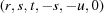
(1) Unroll the Niggli cone by applying the six permutations resulting from interchanging the cell edges and the four possible acute–obtuse angle changes, for an initial set of 24 alternative presentations of each cell, v: v, , , , , , , , , , , , , , , , , , , , , , , .

(2) For each of the 24 resulting cells from step 1, compute the distances to and projections onto each of the 15 five-dimensional Niggli cone boundaries.

(3) For each of the 24 resulting cells from step 1, compute the distances to and projections onto each of the three intersections between the face-diagonal cases and the body-diagonal case in the negative (obtuse angle) portion of the Niggli cone (8F, BF, EF) as well as the distances to and boundary mapping onto the images of those intersections in the positive (acute angle) portion of those intersections. Specifically, for each cell, v, compute the distance, projections and images

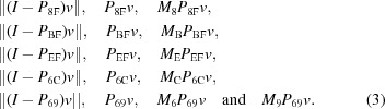(4) For all subsequent distance calculations, also unroll the Niggli standard-form transformations that restrict the Niggli cone to or , by defining

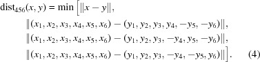This is the minimum distance between two images where one is in the positive branch of the Niggli cone and the other is in the negative branch.

(5) Compute the minimum Euclidean distance from each of the 24 images of the first cell from step 1 to each of the 24 images of the second cell from step 1.

(6) For each of the 15 five-dimensional boundaries and for each of the 576 combinations of one of the 24 images of the first cell and one of the 24 images of the second cell, determine the minimum of the distances computed thus far and the distance going from the first cell to the chosen boundary and then from the boundary to the second cell, treating as equivalent each projection into a boundary and its transformation using the boundary transformation.

(7) For each member of each set of permutations, compute the distance from each permutation to each of the face-diagonal and body-diagonal boundary manifolds. The face-diagonal boundaries are grouped together as three cases (6-7-8, 9-A-B, C-D-E), with two subcases each. In the first three cases these are the full five-dimensional boundaries, and in the subcases these are the four-dimensional boundaries produced by the intersections with the body-diagonal boundary manifold (8F, BF, EF).

(8) For each face-diagonal or body-diagonal boundary manifold, Γ, consider a member from the first set of permutations and from the second set of permutations. Let be the distance from to Γand be the distance from to Γ.

(9) If is less than the minimum distance already found, let be the projection of onto Γ and be the image of that projection under the boundary transformation, and let be the projection of onto Γ and be the image of that projection under the boundary transformation. For the 8F, BF and EF four-dimensional boundaries, use the transformations for the corresponding face-diagonal boundaries (, , ). Compare the minimum distance thus far with { + , , dist, , dist, } and keep the smallest value.

The raw distance in is not sufficient for comparison of lattices of different symmetries and does not consider distances in relationship to the size of experimental errors. The anorthic lattices have the full six degrees of freedom of the space, the monoclinic have four, the orthorhombic have three, the hexagonal and tetragonal have two, and the cubic have one. Multiplying the reported distances by the square root of the number of degrees of freedom provides better comparisons between possible lattices. If one then divides by the experimental error estimate, one gets a dimensionless ‘Z score’.

Computationally, the multiplicities of the combinations used is lower than one might expect because of constant pruning by comparing the distance computed at each stage with the distance to the boundary under consideration. If the boundary distance that was precomputed in step 2 or 3 is larger than the previously computed minimum distance between cells, there is no need to compute path lengths that include that boundary distance.

4. Implementation of the embedding  

BGAOL is a modification of our earlier iteration-based program ITERATE (Andrews & Bernstein, 1988 ▶) using embedding-based distances to search for likely Bravais lattice matches. The only other lattice matching programs that the authors know of that use a metric are BLAF (Macíček & Yordanov, 1992 ▶), DELOS (Zimmermann & Burzlaff, 1985 ▶), XDS (Kabsch, 2010 ▶) and OT-BLD, the lattice matching part of CONOGRAPH (Oishi-Tomiyasu, 2012 ▶). Because of the metric distortions outside the Niggli cone, none of these measures is assured to actually be linear. BLAF uses an (i.e. Manhattan street grid) measure on the metric tensor, while ITERATE and BGAOL use an (i.e. Euclidean) measure. DELOS uses a coarse measure based on ‘cycles’. OT-BLD reports matches using a fractional measure, also based on the metric tensor. XDS uses a ‘quality index’ based on the sum of the extents to which the inequalities of Niggli reduction are not satisfied for components of the metric tensor, essentially an measure of the distance from each Niggli-cone boundary polytope. Table 2 ▶ shows a comparison of BGAOL results with those of other programs, except XDS. Table 3 ▶ shows a com­parison of the BGAOL Z score with the XDS quality indicator.

Table 2. Search results for BGAOL, BLAF, DELOS, OT-BLD and ITERATE for basic beryllium acetate, , ,  Å, , , ° (Himes & Mighell, 1987 ▶).

The BGAOL, BLAF and ITERATE columns show distances in Ų from the probe to the appropriate boundary manifold for the indicated Niggli lattice character in . The BLAF column uses distances versus distances for the others. The DELOS column shows the numbers of cycles of relaxation of the Delaunay reduction needed to find the indicated symmetry. The OT-BLD column is a dimensionless fractional measure of the agreement of metric tensors. The significant differences between the BGAOL and ITERATE values in some cases are a result of the expansion and contraction factors (see the text) when measures are applied outside the Niggli cone.

Lattice character	BGAOL	BLAF	DELOS	OT-BLD	ITERATE
cF	0.067	–	1	1 × 10−5	0.096
tI	0.038	0.014	1	6 × 10−6	0.038
hR	0.065	0.013	1	7 × 10−6	0.076
oF	0.038	–	1	6 × 10−6	0.038
oI	0.019	0.007	1	4 × 10−6	0.018
mI	0.007	0.004	1	1 × 10−6	0.007

Table 3. Partial search results for BGAOL and XDS for the test cell, , ,  Å, , , ° from Kabsch (1993 ▶).

The BGAOL columns show the distance and the degrees-of-freedom weighted Z score, assuming errors of 0.2 in edges and 0.1 on angles, which in this case corresponds to a error estimate of 61.3 Ų. The XDS QI (quality indicator) and scaled QI columns show the raw deviations from Niggli reduction and the same deviations scaled by and capped at 999 as per Kabsch (2013 ▶). Only the three most promising lattice types are shown. The structure solution gave oC. distances are in units of Ų.

Lattice character	distance	BGAOL Z score	XDS QI	Scaled QI
mP	20.138	0.657	1.0	0.13
oC	125.958	3.560	23.8	3.09
mC	125.150	4.085	23.4	3.03

4.1. Distance calculation  

BGAOL distances are calculated using the function NCDIST, which computes the distance between pairs of reduced cells. Bravais lattice determination for a given probe cell consists of finding which boundary polytopes or subspaces among the Bravais lattice subspaces of the Niggli cone are closest to the probe. Constructing and using a cell database requires computing the distance between cells as points in that are arbitrarily far apart. Fig. 2 ▶ illustrates the use of NCDIST to compute distances between well separated points.

Figure 2.

To illustrate distance calculations between arbitrary points, a line was drawn in between an unreduced point close to cF and its reduced image. Each curve shows the distances at 100 points along each line to the corresponding reduced cell of the starting point. The upper curve starts from , ,  Å, , , ° and ends at , ,  Å, , , °. The lower curve starts from , ,  Å, , , ° and ends at , ,  Å, , , °.

4.2. Availability and test results  

A BGAOL-based lattice identification web server is available at http://iterate.sf.net/bgaol. A source kit may also be downloaded from a link on that page.

The prior ITERATE-based lattice identification web server is available at http://www.bernstein-plus-sons.com/software/ITERATE/.

The latest version of the source code of BGAOL is maintained on SourceForge (http://sourceforge.net/) for svn access at

svn checkout

svn://svn.code.sf.net/p/iterate/code/trunk/bgaol

bgaol-code

The source kit contains the test program, Follower.for, that computes the distance for database work as shown in Fig. 2 ▶.

The database code, which will be discussed in a subsequent article, is available from the ‘sauc’ module in the same repository.

Appendix A. The boundary polytopes

The embedding requires an understanding of the space , the process of Niggli reduction, and the resulting Niggli cone and boundaries created thereof on .

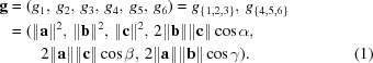
A1. The space G ⁶  

is a reformulation of the crystallographic metric tensor and the ‘Niggli matrix’ (itself a reformulation of the metric tensor) (Andrews & Bernstein, 1988 ▶). A vector in is defined as

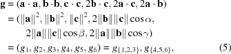where , , are the unit-cell edge vectors, and indicates the dot product. The unit cell is chosen to be primitive.

The notation is used to denote the elements from the full vector.

A2. The Niggli conditions  

The Niggli-reduced cell of a lattice is a unique choice from among the infinite number of alternative cells that generate the same lattice (Niggli, 1928 ▶). A Buerger-reduced cell for a given lattice is any cell that generates that lattice, chosen such that no other cell has shorter cell edges (Buerger, 1960 ▶). Even after allowing for the equivalence of cells in which the directions of axes are reversed or axes of the same length are exchanged, there can be up to five alternative Buerger-reduced cells for the same lattice (Gruber, 1973 ▶). The Niggli conditions allow the selection of a unique reduced cell for a given lattice from among the alternative Buerger-reduced cells for that lattice.

Niggli reduction consists of converting the original cell to a primitive one and then alternately applying two operations: conversion to standard presentation and reduction (Niggli, 1928 ▶; Andrews & Bernstein, 1988 ▶). The convention for meeting the combined Buerger and Niggli conditions is based on increasingly restrictive layers of constraints: if , , , and either or then we have a Niggli-reduced cell, and we are done.

The remaining conditions are imposed when any of the above inequalities becomes an equality or the elements of are not consistently all strictly positive or are not consistently all less than or equal to zero.

The full set of combined Buerger and Niggli conditions in addition to those for the cell edge lengths being minimal is as follows:

The transformations associated with each of these steps are enumerated by Andrews & Bernstein (1988 ▶). Application of these operations must be repeated until all are satisfied.

A3. Notation and boundary polytopes  

We define the manifold of the Niggli-reduced cells in as and refer to it as the ‘Niggli cone’.

The interior of , , is defined as the set of such that there exists such that for all such that .

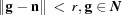The closure of , , is defined as the set of such that for all there exists such that .

The boundary of , , is defined as the set of points in not in .

The boundary of is created by the linear constraints of Niggli reduction and therefore can be decomposed into the union of ‘polytopes’, i.e. flat facets with straight edges.

We distinguish the primary boundary polytopes from their edges, which are also polytopes, by ‘dimension’, which is the number of vectors in a basis for the interior of the polytope.

is a six-dimensional polytope. is a double-ended cone-like region going through the origin to infinity in both directions. The boundary polytopes are flat facets created by the intersections of hyperplanes through the origin. The boundary polytopes are, of course, of lower dimension than . Therefore any randomly selected vector in has a vanishingly small probability of occupying any particular five-dimensional boundary polytope, and it has an even lower probability of occupying one of the lower-dimensional boundary polytopes resulting from the intersections of five-dimensional boundary polytopes. Some boundary polytopes are ‘open’, i.e. while there are Niggli-reduced cells near that boundary, some or all of the points on those boundary polytopes are not themselves Niggli reduced.

Our task is to identify the five-dimensional boundary polytopes that give its shape. Those five-dimensional boundaries and the transforms involved in crossing them generate all the rest of the structure. However, in order to understand the shape of a given five-dimensional boundary polytope, we need the four-dimensional edges that bound it. In order to understand the shape of a given four-dimensional boundary polytope, we need the three-dimensional edges that bound it. In order to understand the shape of a given three-dimensional boundary polytope, we need the two-dimensional edges that bound it. In order to understand the shape of a given two-dimensional boundary polytope, we need the one-dimensional edges that bound it. From this classification we gain a better understanding of the relationships between Bravais lattice types, and, perhaps more importantly, this provides essential information needed to organize computations. Hosoya (1990 ▶) addressed a different, but related, classification. We discuss the relationship between boundary polytope identification, lattice types and Hosoya’s approach in § A10. Hosoya recognized the complexity of boundary identifications for and introduced the use of Monte Carlo searching to clarify the relationships. We apply a Monte Carlo search in Appendix B (Andrews & Bernstein, 1976 ▶; Beltrami, 1873 ▶; Jordan, 1874 ▶; Stewart, 1993 ▶), which is available as supplementary material.2

The reduction steps convert a non-reduced cell into one that has at least one edge shorter than the starting edges, and other steps in the case of equality convert a non-reduced cell into a cell that is more orthogonal than the starting cell. These operations are accomplished by choosing a face or body diagonal to replace one of the cell edges. The conditions added to remove the ambiguities in the case of equalities allow for a unique choice of Niggli cell in all cases but thereby create complex boundary conditions (Andrews & Bernstein, 1988 ▶). For example, the cell edge equalities in equations (7) and (8) create boundary polytopes across which elements of both and are exchanged, while equations (3) and (4) create boundary polytopes across which edges are exchanged for face diagonals.

A boundary polytope does not necessarily consist entirely of Niggli-reduced cells but can contain non-Niggli-reduced cells including nearly reduced cells as well. We define a boundary polytope as a subset of for which there is an associated matrix such that for all points there exists such that for all where , . Each boundary polytope is a portion of the boundary for which there is a single transformation matrix that maps the nearby non-Niggli-reduced cells to Niggli-reduced cells. This is not necessarily a mapping back to the starting point, or even to a point near the starting point, not even for points on the boundary polytope itself. We look for point-by-point invariance in defining special-position subspaces in § A4.

Each boundary polytope has an associated ‘projector’ , which is the linear transformation that maps an arbitrary to the point closest to g in the hyperplane containing . It is important to understand that may not be Niggli reduced or even close to the Niggli cone.

A4. Special-position subspaces  

In an analysis of symmetry, special positions play an important role. A special position is a point invariant under a symmetry transformation, an eigenvector, of eigenvalue 1, of the transformation. We define a special-position subspace of a boundary polytope as the intersection of the eigenspace of eigenvalue 1 of with the boundary polytope. Formally, for a boundary polytope with associated transformation matrix , the special-position subspace is defined as the set of points such that . In the case of boundary polytopes associated with a transformation matrix that goes from the all-acute case to the all-obtuse case or vice versa, there cannot be any Niggli-reduced special-position subspace, because the axial planes of the subspace are excluded from the all-acute case. As we will see, while the special-position subspaces of the boundary polytopes are not needed in order to classify the primitive lattice types, they come into play in classifying the non-primitive lattice types.

If we have two boundary polytopes , , we denote the intersection of the closure of and the closure of as . Note that intersection is a commutative operation, i.e. .

Because we have restricted the boundary polytope in this article to have only one associated matrix, we use the notation for . In general, an infinite number of higher-dimensional polytopes will intersect in . We distinguish such a higher-dimensional polytope as . Thus .

A5. The 15 five-dimensional boundary polytopes  

The 15 five-dimensional boundary polytopes and their special-position subspaces may be organized as shown in Table 1 ▶, in which we use the hexadecimal digits 1 through F as identifiers. For each five-dimensional boundary polytope in Table 1 ▶ having a nontrivial special-position subspace, we designate the particular choice of higher-dimensional polytope intersecting in as . See § A5.3 for a concrete example.

In the discussions of the 15 five-dimensional boundary polytopes below, we give the condition being satisfied, the right-handed representation of the boundary transformation cell edge by cell edge, a matrix representation of the same boundary transformation and a matrix representation of a projector into the hyperplane of that boundary. Note that both a right-handed representation and its negative (left-handed) representation would map into the same representation.

A5.1. Equal-cell-edge case  

Cases 1 and 2 arise when two cell edges have equal length. In this section some scalar components are in bold face to direct the attention of the reader to values that are changing. The conditions of Niggli reduction impose a secondary condition on the associated angles for those two edges that resolves the ambiguity in ordering them. For example, in case 1, () and the Niggli-reduced vector produces the same lattice as , which is not Niggli reduced if and have different values. In going from Niggli-reduced cells near U to Niggli-reduced cells near V (e.g. by decreasing slightly), we are crossing a boundary polytope with a discontinuity in each of and (Andrews & Bernstein, 1988 ▶). We may represent the transformation that takes U into V at the first boundary polytope by the matrix that maps U into V and the projector that maps any vector into the boundary polytope.

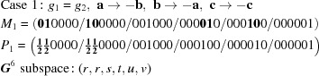Similarly, for case 2, (), and are exchanged, yielding

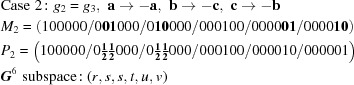The remaining equal-cell-edge case, in which (), is only considered under Niggli reduction when and , which is a combination of case 1 and case 2. This requires two simultaneous five-dimensional constraints, thereby making a four-dimensional rather than a five-dimensional case.

The special-position subspaces and are obtained by adding the constraints and , respectively.

A5.2. Ninety degree case  

Cases 3, 4 and 5 arise when a reduced cell angle is 90°. In those cases, the remaining cell angles both can be replaced by their supplements. This changes the sign of .

In each 90° case, the special-position subspace consists of 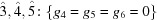, i.e. the primitive orthorhombic case, and we take , , .

A5.3. Face-diagonal case  

Cases 6 through E are all face-diagonal cases, in which a cell edge is equal in length to a face diagonal. Some complexity arises in the analysis because, unlike Delaunay reduction, Niggli reduction permits non-obtuse angles. We can always change the sign of any two elements of by changing the direction of the cell edge involved with those two elements. For example, if we transform to then, while remains unaffected, the signs of each of and will change. Thus we can transform a cell having three acute angles to a cell having one acute angle and two obtuse angles, and we can transform a cell having three obtuse angles to a cell having one obtuse angle and two acute angles. The complete list of possible sign changes in by changing the directions of axes are

Unless one of the angles is 90° (which introduces a zero into ), we cannot ordinarily transform a Niggli-reduced cell with all-acute angles to one with all-obtuse angles by changing the directions of axes, nor can we transform a Niggli-reduced cell with all-obtuse angles to one with all-acute angles by changing the directions of the axes. Note that changing the direction of all three axes has no effect because all the sign changes cancel.

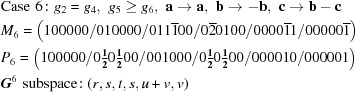
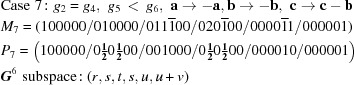
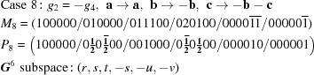
The face-diagonal cases do include cases in which transformations from, for example, to do occur. Let us look in detail at cases 6 and 7, .

Thus transforming to will not change the cell edge lengths. In this case, , and are, of course, unchanged and

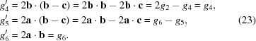This shows that a single element of , , will change sign depending on the sign of . Cases 6 and 7 cannot start from the all-obtuse case because and because must be nonnegative. Starting from an all-acute case, , we will remain in the all-acute case if is greater than or equal to but go to one having one obtuse angle (not reduced) if is less than . We then change to having all-obtuse angles, , by reversing the direction of b. The resulting matrices in these face-diagonal cases are

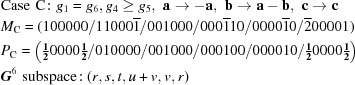
The special-position subspaces of the face-diagonal boundary polytopes 6, 8, 9, B, C and E are empty because such a special position would require a common point in the all-acute and all-obtuse cases that only meet at the axial planes of the subspace, which are excluded from the all-acute case. For cases 7, A and D there are non-trivial special-position subspaces. An invariant point in case 7 would have to satisfy or . Thus we define and similarly define and .

A5.4. Body-diagonal case  

There is only one five-dimensional body-diagonal case, :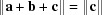

In order to have a special-position subspace in case F, in addition to , we need (from the fourth and fifth rows of ) and , from which we have , from which we take . This is equivalent to , i.e. that the shorter b-face diagonal is the same length as the shorter a-face diagonal.

A6. The four-dimensional boundary polytopes  

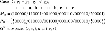
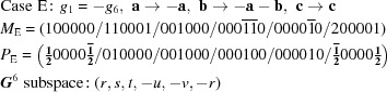
The four-dimensional boundary polytopes are created by the intersection of two five-dimensional boundary polytopes. Certain intersections are degenerate. For example, cases 8, B, E and F are restricted to the branch of the boundary of the Niggli cone, while cases 6, 7, 9, A, C and D are restricted to the branch. More subtly, cases 6 and 7 require , maximizing , forcing and which would conflict with cases A and D. Only cases 9 and C, taken to their boundaries with A and D, respectively, are possible. Those boundaries are designated 9A and CD, respectively. Similarly, cases 9 and A maximize , which would conflict with case 7 and force 6 to the 67 boundary, and cases C and D maximize , which would conflict with case 6 except at the 67 boundary. Thus cases 6A, 7A, 6D, 7D, 79, 7A and 6C actually are the lower dimension cases 69A, 79A, 6CD, 7CD, 79A, 79A and 6CD, respectively. This process can result in three- or even two-dimensional boundary polytopes from the intersection of two five-dimensional boundary polytopes (see below). After excluding the cases that involve any of , there are 55 four-dimensional cases as shown in the supporting information (Appendix B, Table 3). The relative populations for all the two-dimensional boundary polytopes except 26, 28, 2A and 2D have Z scores above −1. The Z scores for those four cases range from −1.1 down to −1.9. (See the supplementary materials for a discussion of Z scores).

The edges of the five-dimensional polytopes can be read directly from Appendix B, Table 3. For example the 6 polytope is bounded by 16, 26, 56, 67 and 69, and the F polytope is bounded by 1F, 2F, 8F, BF and EF. It is important to note that the polytopes 1, 2, 3, 4 and 5 extend into the boundaries of both the and the branches of . Even though the polytopes 3, 4 and 5 do not contain any valid Niggli-reduced cells, they are part of both branches of even for .

A7. The three-dimensional boundary polytopes  

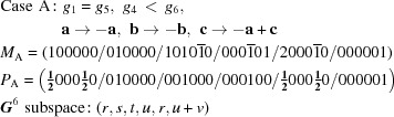
The three-dimensional boundary polytopes are created by the intersection of three five-dimensional boundary polytopes. In some cases the boundary polytope is better represented by a fourfold intersection. The boundary polytope 34CD is equivalent to 34C and 34D, 359A is equivalent to 359 and 35A, 4567 is equivalent to 456 and 457, 679C is equivalent to 69C and 79C, and 9ACD is equivalent to 9AD and ACD. These are ‘flat boundary intersection’ cases in which one side of the flat boundary intersection implies the other. On the other hand 126 and 127, 12A and 129, 12C and 12D, 2AD and 29C, and 69C and 79C are distinct rather than equivalent pairs of flat boundary intersections. Six twofold intersections of five-dimensional boundary polytopes (6A, 6C, 79, 7D, 9D and AC) result in three-dimensional boundary polytopes, rather than in four-dimensional boundary polytopes. In each case both boundary polytopes have mismatched partners from ‘flat boundary intersections’. Let us examine the 6A case in detail, elaborating on the discussion of the four-dimensional boundary polytopes above.

Cases 6 and A are and , and and , respectively. For intersections, we use the closures of the boundary polytopes, so we have the closure of A as and . The Niggli cone itself imposes the additional restrictions and , but from 6, , and from the closure of A, , so we have

and from the Niggli reduction conditions

Thus and , meaning that, in addition to satisfying the constraints of case A, we also satisfy the constraints of case 9, and . Thus case 6A is actually case 69A, producing a true three-dimensional boundary polytope from the intersection of two five-dimensional boundary polytopes owing to the additional constraints of Niggli reduction. As we will see in the discussion of the two-dimensional boundary polytopes, the Niggli reduction constraints can result in shedding one or more degrees of freedom, allowing some twofold intersections of five-dimensional boundary polytopes to result in two-dimensional boundary polytopes.

After excluding the cases that involve any of , there are 79 cases as shown in Appendix B, Table 4. The relative populations for all the three-dimensional boundary polytopes have Z scores greater than −1.1.

For completeness, if one wished to include the boundary polytope with it would be considered in the three-dimensional polytopes. In , forces , , leaving only three degrees of freedom at . Note that is of even lower dimension, one, because forces as well as , leaving only one degree of freedom (). is just the origin.

A8. The two-dimensional boundary polytopes  

The two-dimensional boundary polytopes are, in general, created by the intersection of four five-dimensional boundary polytopes, but several well populated fourfold intersections result in three-dimensional boundary polytopes rather than two-dimensional boundary polytopes. Several fourfold intersections are most naturally presented as higher multiplicity intersections, and in some cases the intersection of as few as two five-dimensional boundary polytopes is sufficient to create a two-dimensional boundary polytope. After excluding the cases that involve any of , there are 55 cases as shown in Appendix B, Table 5. The combination of seven boundary polytopes 1679ACD is the hexagonal rhombohedral hR, lattice character 9, Roof/Niggli symbol 49B, subspace . Alternatively, lattice character 9 can be viewed as any of 81 other intersections, including two twofolds (6D, 7A), 18 threefolds (179, 16A, 16C, 16D, 17A, 17D, 19D, 1AC, 67A, 67D, 69D, 6AC, 6AD, 6CD, 79A, 79D, 7AC, 7AD), 33 fourfolds (1679, 167A, 167C, 167D, 169A, 169C, 169D, 16AC, 16AD, 16CD, 179A, 179C, 179D, 17AC, 17AD, 17CD, 19AC, 19AD, 19CD, 1ACD, 679A, 679D, 67AC, 67AD, 67CD, 69AC, 69AD, 69CD, 6ACD, 79AC, 79AD, 79CD, 7ACD), 21 fivefolds (1679A, 1679C, 1679D, 167AC, 167AD, 167CD, 169AC, 169AD, 169CD, 16ACD, 179AC, 179AD, 179CD, 17ACD, 19ACD, 679AC, 679AD, 679CD, 67ACD, 69ACD, 79ACD) and seven sixfolds (1679AC, 1679AD, 1679CD, 167ACD, 169ACD, 179ACD, 679ACD), and is a very highly populated two-dimensional boundary polytope. If we exclude this case, the remaining 54 cases have Z scores ranging from −1.36 (for 1456) to 0.84 (for 123E) to 2.75 (for 29ACD).

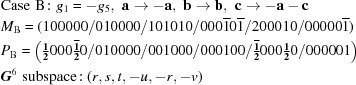
Let us consider how one of the twofolds, 6D, results in only two degrees of freedom. Cases 6 and D are and , and and , respectively. The closure of D is and , and Niggli reduction requires , from which it follows that

and therefore

creating the subspace , i.e. two degrees of freedom.

A9. The one-dimensional boundary polytopes  

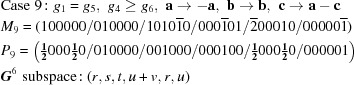
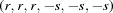
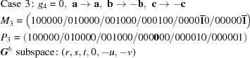
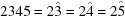
There are 14 distinct one-dimensional boundary polytopes, with many equivalent presentations. The most complex situation is best presented as an eightfold intersection, 12679ACD, i.e. , which is the face-centered cubic . There are 81 other equivalent presentations of the face-centered cubic, inherited from the sevenfold intersection hexagonal rhombohedral discussed above by adding case 2 to each of those presentations, thereby providing two threefolds for the face-centered cubic case (26D and 27A). 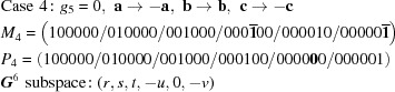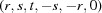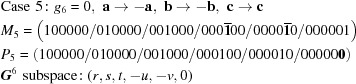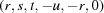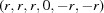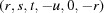The remaining 13 one-dimensional boundary polytopes are 12345 , 1234CD (equivalent to 1234C, 1234D, 123CD, 124CD), 1234E , 12359A (equivalent to 12359, 1235A, 1239A, 1259A), 1235B , 123AD , 123BEF (equivalent to 123BE, 123BF, 123EF, 12BEF, 23BEF), 124567 (equivalent to 12456, 12457, 12467, 12567), 12458 , 1247C , 1248EF (equivalent to 1248E, 1248F, 124EF, 128EF), 12569 and 1258BF (equivalent to 1258B, 1258F, 125BF, 128BF).

These 14 one-dimensional boundary polytopes of correspond exactly to the 14 vertices of the hyperpolyhedra given by Gruber (1997 ▶, Table 1) for which none of are zero. The 14 that match are a confirmation of the completeness of this analysis. Owing to the distortion introduced by projection, the rejection of the cases for which any of are zero is important in preserving the metric for incommensurate edges near the origin.

If we exclude the highly populated face-centered cubic, the Z scores for the relative populations of the remaining 13 one-dimensional boundary polytopes range from more than −1.1 for 12569 to 1.44 for 123BEF.

A10. Relationship between boundary polytopes and lattice type  

‘Lattice characters’ provide a finer-grained division of lattice type than the 14 Bravais lattice types (International Tables for Crystallography, Vol. A, Burzlaff et al., 1992 ▶). In order to understand the relationship between the 216 boundary polytopes and the 44 lattice characters in International Tables, we use combinations of the 15 five-dimensional boundary polytopes and of the special-position subspaces of those polytopes. There are multiple alternative representations of some of the lattice characters. We discuss some of them below.

We refer to Roof’s redrawn Niggli figure identifiers (Roof, 1967 ▶) as ‘Roof/Niggli symbols’. We may associate the Roof/Niggli symbols, lattice characters and Bravais lattice types with the indicated subspaces of and combinations of boundary polytopes and special conditions as shown in Table 4 ▶. The triclinic lattice characters 31 and 44 are not included because no boundary polytopes are needed for the triclinic case as they fill the Niggli-reduced cone.

Table 4. Roof/Niggli symbol, International Tables (IT) lattice character, Bravais lattice type, subspace (Andrews & Bernstein, 1988 ▶) and boundary polytope.

Roof/Niggli symbol	IT lattice character	Bravais lattice type	subspace	boundary polytope
44A	3	cP
44C	1	cF		12679ACD
44B	5	cI
45A	11	tP
45B	21	tP
45D	6	tI
45D	7	tI
45C	15	tI		158BF
45E	18	tI
48A	12	hP		134E
48B	22	hP		2458
49C	2	hR
49D	4	hR
49B	9	hR		1679ACD
49E	24	hR
50C	32	oP
50D	13	oC		134
50E	23	oC		245
50A	36	oC		35B
50B	38	oC		34E
50F	40	oC		458
51A	16	oF
51B	26	oF
52A	8	oI		12F
52B	19	oI		29C = 2AD
52C	42	oI		58BF
53A	33	mP		35
53B	35	mP		45
53C	34	mP		34
55A	10	mC
55A	14	mC
57B	17	mC		1F
55B	20	mC
55B	25	mC
57C	27	mC		9C = AD
56A	28	mC
56C	29	mC
56B	30	mC
54C	37	mC		5B
54A	39	mC		4E
54B	41	mC		58
57A	43	mC

The primitive Bravais lattice types have a simple relationship to the boundary polytopes. The primitive cubic, which has one degree of freedom as a subspace, is the intersection of five five-dimensional boundary polytopes. The primitive tetragonal and primitive hexagonal lattice types each have two degrees of freedom as subspaces and each is the intersection of four five-dimensional boundary polytopes. The primitive ortho­rhombic lattice type has three degrees of freedom as a subspace and is the intersection of three five-dimensional boundary polytopes. The primitive monoclinic lattice types each have four degrees of freedom as subspaces, and each is the intersection of two five-dimensional boundary polytopes.

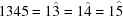
The combination of eight boundary polytopes 12679ACD (equivalent to the threefold combinations 26D and 27A) is the face-centered cubic cF, lattice character 1, Roof/Niggli symbol 44C, subspace (Andrews & Bernstein, 1988 ▶). Alternatively, cF can be viewed as any of , or and of several other intersections. As one would expect from the large number of intersecting boundary polytopes, this is a very complex region of and will be the subject of a later article.

The one-dimensional combinations of six boundary polytopes 1234CD (equivalent to the fivefolds 1234C, 1234D, 123CD, 124CD), 12359A (equivalent to the fivefolds 12359, 1235A, 1239A, 1259A), 123BEF (equivalent to the fivefolds 123BE, 123BF, 123EF, 12BEF, 23BEF), 124567 (equivalent to the fivefolds 12456, 12457, 12467, 12567), 1248EF (equivalent to the fivefolds 1248E, 1248F, 124EF, 128EF) and 1258BF (equivalent to the fivefolds 1258B, 1258F, 125BF, 128BF) form the subspaces

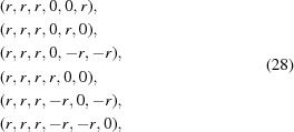of which none are Niggli-reduced and which are therefore a set of open-boundary polytopes.

Most of the 216 boundary polytopes are non-Niggli-reduced open-boundary polytopes of the Niggli region. Therefore only two of the fivefold boundary polytopes, five of the fourfold boundary polytopes, eight of the threefold boundary polytopes and 11 of the twofold boundary polytopes correspond directly to lattice characters. None of the single five-dimensional boundary polytopes correspond to lattice characters.

We are working from the boundary polytopes, looking for the resulting symmetries. Hosoya (1990 ▶) started, instead, from the three highest-symmetry lattice types (the three cubics), added the lower-symmetry primitive hexagonal lattice type, and inferred boundary polytopes from the symmetries, having to treat open-boundary polytopes as if they were Niggli reduced. The resulting six boundary polytopes of the three cubics and the primitive hexagonal restated in terms of are given in Table 5 ▶.

Table 5. The Hosoya boundary polytopes of the three cubic lattice types and the primitive hexagonal in terms of .

Hosoya1
Hosoya2
Hosoya3
Hosoya4	, the special-position subspace of case 1
Hosoya5	, the special-position subspace of case 2
Hosoya6	, the special-position subspace of case D

A11. Boundary polytope summary  

The widespread use of Niggli reduction in crystallography implies that it should be thoroughly understood. Robust identification of Bravais lattices and lookup of unit-cell parameters in databases would be improved if a successful embedding of the Niggli space could be achieved. We have investigated and enumerated the several kinds of boundary polytopes on the Niggli cone and enumerated the transformations and projectors specific to each. While other, related, work has often used three-dimensional sections, our work natively addresses the boundary polytopes and transformations in the Euclidean space . The single point of view and the simple linear algebra involved makes the presentation more consistent.

Some unexpected complexities have been encountered, such as the occurrence of one boundary polytope that is the intersection of eight five-dimensional boundary polytopes, a fruitful area for further investigation.

References

- Andrews, L. C. & Bernstein, H. J. (1976). Acta Cryst. A32, 504–506.
- Andrews, L. C. & Bernstein, H. J. (1988). Acta Cryst. A44, 1009–1018.
- Andrews, L. C., Bernstein, H. J. & Pelletier, G. A. (1980). Acta Cryst. A36, 248–252.
- A Society of Gentlemen in Scotland (1771). Editor. Encyclopedia Britannica, or, a Dictionary of Arts and Sciences, Compiled upon a New Plan, Vol. II(54), p. 677. Edinburgh: A. Bell and C. Macfarquhar.
- Azaroff, L. V. & Buerger, M. J. (1958). The Powder Method in X-ray Crystallography, ch. 11, pp. 124–159. New York: McGraw-Hill.
- Beltrami, E. (1873). G. Mat. Uso Studenti Univ. 11, 98–106.
- Buerger, M. J. (1960). Z. Kristallogr. 113, 52–56.
- Burzlaff, H., Zimmermann, H. & de Wolff, P. M. (1992). International Tables for Crystallography, Vol. A, edited by T. Hahn, ch. 9, pp. 734–744. Dordrecht: Kluwer Academic Publishers.
- Byram, S. K., Campana, C. F., Fait, J. & Sparks, R. A. (1996). J. Res. NIST, 101, 295–300. [DOI] [PMC free article] [PubMed]
- Delaunay, B. N. (1932). Z. Kristallogr. 84, 109–149.
- Gruber, B. (1973). Acta Cryst. A29, 433–440.
- Gruber, B. (1997). Acta Cryst. A53, 505–521.
- Gruber, B. (2006). International Tables for Crystallography, Vol. A, 1st online ed., edited by T. Hahn, ch. 9.3, pp. 756–760. Chester: International Union of Crystallography.
- Helgason, S. (1962). Differential Geometry and Symmetric Spaces New York, London: Academic Press.
- Himes, V. L. & Mighell, A. D. (1987). Acta Cryst. A43, 375–384.
- Hosoya, M. (1990). Bull. Coll. Sci. Univ. Ryukyus, 50, 1–13.
- Hosoya, M. (2000). Acta Cryst. A56, 259–263. [DOI] [PubMed]
- Jordan, C. (1874). J. Math. Pures Appl. Deuxiéme Ser. 19, 35–54.
- Kabsch, W. (1993). J. Appl. Cryst. 26, 795–800.
- Kabsch, W. (2010). Acta Cryst. D66, 133–144. [DOI] [PMC free article] [PubMed]
- Kabsch, W. (2013). Personal communication.
- Macíček, J. & Yordanov, A. (1992). J. Appl. Cryst. 25, 73–80.
- McGill, K. J., Mojgan, A., Karakasheva, M. T., Andrews, L. C. & Bernstein, H. J. (2014). J. Appl. Cryst. 47, 360–354. [DOI] [PMC free article] [PubMed]
- Minor, W. & Otwinowski, Z. (1997). Crystallographic Computing 7. Proceedings from the Macromolecular Crystallography Computing School. Chester: International Union of Crystallography.
- Nash, J. (1956). Ann. Math. 63, 20–63.
- Niggli, P. (1928). Krystallographische und Strukturtheoretische Grundbegriffe, Handbuch der Experimentalphysik, Vol. 7(1). Leipzig: Akademische Verlagsgesellschaft.
- Oishi-Tomiyasu, R. (2012). Acta Cryst. A68, 525–535. [DOI] [PubMed]
- Roof, R. B. Jr (1967). A Theoretical Extension of the Reduced-Cell Concept in Crystallography Report No. LA-4038, TID-4500. Los Alamos Scientific Laboratory, New Mexico, USA. http://lib-www.lanl.gov/cgi-bin/getfile?00378045.pdf.
- Seeber, L. A. (1831). Untersuchungen über die Eigenschaften der positiven ternæren quadratischen Formen, Vol. 1. Mannheim: Tobias Loeffler.
- Selling, E. (1874). J. Reine Angew. Math. 1874, 143–229.
- Stewart, G. W. (1993). SIAM Rev. pp. 551–566.
- Toby, B. (1994). Personal communication.
- Von Laue, M. (1952). International Tables for X-ray Crystallography, Vol. I, edited by N. F. M. Henry & K. Lonsdale, pp. 1–5. Birmingham: Kynoch Press.
- Zimmermann, H. & Burzlaff, H. (1985). Z. Kristallogr. 170, 241–246.
Associated Data
This section collects any data citations, data availability statements, or supplementary materials included in this article.
Supplementary Materials
Appendix B. DOI: 10.1107/S1600576713031002/kk5144sup1.pdf