

Abstract
We propose a new method to maximize biomarker efficiency for detecting anatomical change over time in serial MRI. Drug trials using neuroimaging become prohibitively costly if vast numbers of subjects must be assessed, so it is vital to develop efficient measures of brain change. A popular measure of efficiency is the minimal sample size (n80) needed to detect 25% change in a biomarker, with 95% confidence and 80% power. For multivariate measures of brain change, we can directly optimize n80 based on a Linear Discriminant Analysis (LDA). Here we use a supervised learning framework to optimize n80, offering two alternative solutions. With a new medial surface modeling method, we track 3D dynamic changes in the lateral ventricles in 2065 ADNI scans. We apply our LDA-based weighting to the results. Our best average n80—in two-fold nested cross-validation—is 104 MCI subjects (95% CI: [94,139]) for a 1-year drug trial, and 75 AD subjects [64,102]. This compares favorably with other MRI analysis methods. The standard “statistical ROI” approach applied to the same ventricular surfaces requires 165 MCI or 94 AD subjects. At 2 years, the best LDA measure needs only 67 MCI and 52 AD subjects, versus 119 MCI and 80 AD subjects for the stat-ROI method. Our surface-based measures are unbiased: they give no artifactual additive atrophy over three time points. Our results suggest that statistical weighting may boost efficiency of drug trials that use brain maps.
Keywords: Linear Discriminant Analysis, Shape analysis, ADNI, Lateral ventricles, Alzheimer’s disease, Mild cognitive impairment, Biomarker, Drug trial, Machine learning
Introduction
Biomarkers of Alzheimer’s disease based on brain imaging must offer relatively high power to detect longitudinal changes in subjects scanned repeatedly over time (Cummings, 2010; Ross et al., 2012; Wyman et al., accepted for publication). Even so, recruitment and scanning are costly, and a drug trial may not be attempted at all, unless disease-slowing effects can be detected in an achievable sample size, and in a reasonable amount of time. Imaging measures from standard structural MRI show considerable promise. Their use stems from the premise that longitudinal changes may be more precisely and reproducibly measured with MRI than comparable changes in clinical, CSF, or proteomic assessments; clearly, whether that is true depends on the measures used. Brain measures that are helpful for diagnosis, such as PET scanning to assess brain amyloid or CSF measures of amyloid and tau proteins, may not be stable for longitudinal trials that aim to slow disease progression. As a result, there is interest in testing the reproducibility of biomarkers, as well as methods to weight or combine them to make the most of all the available measures (Yuan et al., 2012).
Recent studies have tested the reproducibility and accuracy of a variety of MRI-derived measures of brain change. Several are highly correlated with clinical measures, and can predict future decline on their own, or in combination with other relevant measures. Although not the only important consideration, some analyses have assessed which MRI-based measures show greatest effect sizes for measuring brain change over time, while avoiding issues of bias and asymmetry that can complicate longitudinal image analysis (Fox et al., 2011; Holland et al., 2011; Hua et al., 2011), and while avoiding removing scans from the analysis that may lead to unfairly optimistic sample size estimates (Hua et al., 2012; Wyman et al., accepted for publication). Promising MRI-based measures include the brain boundary shift integral (Leung et al., 2012; Schott et al., 2010), the ventricular boundary shift integral (Schott et al., 2010) and measures derived from anatomical segmentation software such as Quarc or FreeSurfer, some of which have been recently modified to handle longitudinal data more accurately (Fischl and Dale, 2000; Holland and Dale, 2011; Reuter et al., 2012; Smith et al., 2002).
Although several approaches are possible, one type of power analysis, advocated by the ADNI Biostatistics Core (Beckett, 2000), is to estimate the minimal sample size required to detect, with 80% power, a 25% reduction in the mean annual change, using a two-sided test and standard significance level α=0.05 for a hypothetical two-arm study (treatment versus placebo). The estimate for the minimum sample size is computed from the formula below. denotes the annual change (average across the group) and refers to the variance of the annual rate of change.
| (1) |
Here zα is the value of the standard normal distribution for which P [Z<zα]=α. The sample size required to achieve 80% power is commonly denoted by n80. Typical n80s for competitive methods are under 150 AD subjects and under 300 MCI subjects; the larger numbers for MCI reflect the fact that brain changes tend to be slower in MCI than AD and MCI is an etiologically more heterogeneous clinical category. For this reason, it is harder to detect a modification of changes that are inherently smaller, so greater sample sizes are needed to guarantee sufficient power to detect the slowing of disease. In addition, there is some interest in prevention trials targeting cognitively normal subjects who are at risk for AD by virtue of a family history or specific genetic profile (e.g., ApoE genotype); for these and other cohorts, efficiency must be a high priority, and measures that can distinguish AD from normal aging may be unable to track subtle changes efficiently in controls.
Many algorithms can detect localized or diffuse changes in the brain, creating detailed 3D maps of changes (Avants et al., 2008; Leow et al., 2007; Shi et al., 2009), but the detail in the maps they produce is often disregarded when making sample size estimates according to Eq. (1), as the formula expects a single, univariate measure of change. In other words, it requires a single number, or ‘numeric summary’ to represent all the relevant changes occurring within the brain. To mitigate this problem, Hua et al. (2009) defined a “statistical ROI” based on a small sample of AD subjects by thresholding the t-statistic of each feature (voxel) and summing the relevant features over the ROI; this approach was initially advocated in the FDG-PET literature to home in on regions that show greatest effects (Chen et al., 2010). In spirit, the statistical ROI is a rudimentary supervised learning approach, as it finds regions that show detectable effects in a training sample, and uses them to empower the analysis of future samples; the samples used are non-overlapping and independent, to avoid circularity. However, a simple threshold-based masking is known to potentially eliminate useful features, as binarization loses a lot of the information present in continuous weights (Duda et al., 2001). While many studies have used machine learning to predict the progression of neurodegenerative diseases and differentiate diagnostic groups such as AD, MCI, and controls (Kloppel et al., 2012; Kohannim et al., 2010; Vemuri et al., 2008), we found no attempts in the literature that used learning to directly optimize power to detect brain change. The closest work is perhaps that of Hobbs et al. (2010). In this paper, SVM was used to separate subjects with Huntington’s disease from controls, and the resulting score used to calculate sample size estimates. Our goal here was to generalize the very simple binary feature weighting in the stat-ROI approach by directly maximizing the power estimate in a training sample. A linear weighting that optimizes Eq. (1) directly, while using multiple features at once, is exactly analogous to a one-class Linear Discriminant Analysis (LDA), discriminating the disease class from an imaginary sample of zero mean whose covariance is identical to the disease group. We propose two approaches to perform this task: one optimizes Eq. (1) directly by Tikhonov regularization; the other is based on principal components analysis (PCA).
A common criticism of the power analysis provided by Eq. (1) is that it does not take into consideration normal aging in non-high risk healthy subjects (Holland et al., 2011). To mitigate this, several researchers have proposed simply subtracting the mean value of the change computed from controls, while using only the diseased subjects for a variance estimate. This same issue can be directly addressed in the LDA framework. In this case, the problem reduces to the usual 2-class LDA classification, except that the covariance structure is based on the diseased group only, and no assumption of homoscedasticity (equality of variance) is made. This modification is particularly useful for revealing subtle disease-specific atrophy in regions that also change, to some extent, with normal aging.
We apply our LDA approach to maps of surface-based “thickness” changes in the lateral ventricles over intervals of 1 and 2 years after a baseline scan. The analyses are performed on MRI scans from the ADNI-1 dataset. Using two follow-up time points, where available, in addition to the baseline scan allows us to estimate the presence of any longitudinal bias, or intransitivity, which has been a subject of controversy in recent ADNI studies (Hua et al., 2011, 2012; Thompson and Holland, 2011). To register the ventricles and compute radial thickness measures, we modify a recently proposed (Gutman et al., 2012) medial curve algorithm for longitudinal registration. Our general approach is to compute a single continuous curve skeleton and use the curve to induce feature functions on the surface. Shape registration is then performed parametrically by minimizing the L2 difference (summed squared difference) between corresponding feature functions of a pair of shapes.
We note that ventricular expansion is not specific to AD and the ventricles are often also abnormally enlarged in vascular dementia, frontotemporal lobar degeneration, traumatic brain injury, Huntington’s disease, and schizophrenia, among other conditions. Even so, using detailed surface-based maps of the location of expansion—in conjunction with a modified 2-class LDA—helps to reveal aspects of ventricular expansion associated with the progression of Alzheimer’s disease.
Materials and methods
Alzheimer’s Disease Neuroimaging Initiative
Data used in the preparation of this article were obtained from the Alzheimer’s Disease Neuroimaging Initiative (ADNI) database (adni.loni.ucla.edu). The ADNI was launched in 2003 by the National Institute on Aging (NIA), the National Institute of Biomedical Imaging and Bioengineering (NIBIB), the Food and Drug Administration (FDA), private pharmaceutical companies and non-profit organizations, as a $60 million, 5-year public-private partnership. The primary goal of ADNI has been to test whether serial magnetic resonance imaging (MRI), positron emission tomography (PET), other biological markers, and clinical and neuropsychological assessment can be combined to measure the progression of mild cognitive impairment (MCI) and early Alzheimer’s disease (AD). Determination of sensitive and specific markers of very early AD progression is intended to aid researchers and clinicians to develop new treatments and monitor their effectiveness, as well as lessen the time and cost of clinical trials.
The Principal Investigator of this initiative is Michael W. Weiner, MD, VA Medical Center and University of California, San Francisco. ADNI is the result of efforts of many co-investigators from a broad range of academic institutions and private corporations, and subjects have been recruited from over 50 sites across the U.S. and Canada. The initial goal of ADNI was to recruit 800 adults, ages 55 to 90, to participate in the research, approximately 200 cognitively normal older individuals to be followed for 3 years, 400 people with MCI to be followed for 3 years and 200 people with early AD to be followed for 2 years. For up-to-date information, see www.adni-info.org.
Longitudinal brain MRI scans (1.5 T) and associated study data (age, sex, diagnosis, genotype, and family history of Alzheimer’s disease) were downloaded from the ADNI public database (http://www.loni.ucla.edu/ADNI/Data/) on July 1st 2012. The first phase of ADNI, i.e., ADNI-1, was a five-year study launched in 2004 to develop longitudinal outcome measures of Alzheimer’s progression using serial MRI, PET, biochemical changes in CSF, blood and urine, and cognitive and neuropsychological assessments acquired at multiple sites similar to typical clinical trials.
All subjects underwent thorough clinical and cognitive assessment at the time of scan acquisition. All AD patients met NINCDS/ADRDA criteria for probable AD (McKhann et al., 1984). The ADNI protocol lists more detailed inclusion and exclusion criteria (Mueller et al., 2005a, 2005b), available online http://www.nia.nih.gov/alzheimers/clinical-trials). The study was conducted according to the Good Clinical Practice guidelines, the Declaration of Helsinki and U.S. 21 CFR Part 50-Protection of Human Subjects, and Part 56-Institutional Review Boards. Written informed consent was obtained from all participants before performing experimental procedures, including cognitive testing.
MRI acquisition and image correction
All subjects were scanned with a standardized MRI protocol developed for ADNI (Jack et al., 2008). Briefly, high-resolution structural brain MRI scans were acquired at 59 ADNI sites using 1.5 Tesla MRI scanners (GE Healthcare, Philips Medical Systems, or Siemens). Additional data was collected at 3-T, but is not used here as it was only collected on a subsample that is too small for making comparative assessments of power. Using a sagittal 3D MP-RAGE scanning protocol, the typical acquisition parameters were repetition time (TR) of 2400 ms, minimum full echo time (TE), inversion time (TI) of 1000 ms, flip angle of 8°, 24 cm field of view, 192×192×166 acquisition matrix in the x-, y-, and z-dimensions, yielding a voxel size of 1.25×1.25×1.2 mm3, later reconstructed to 1 mm isotropic voxels. For every ADNI exam, the sagittal MP-RAGE sequence was acquired a second time, immediately after the first using an identical protocol. The MP-RAGE was run twice to improve the chance that at least one scan would be usable for analysis and for signal averaging if desired.
The scan quality was evaluated by the ADNI MRI quality control (QC) center at the Mayo Clinic to exclude failed scans due to motion, technical problems, significant clinical abnormalities (e.g., hemispheric infarction), or changes in scanner vendor during the time-series (e.g., from GE to Philips). Image corrections were applied using a standard processing pipeline consisting of four steps: (1) correction of geometric distortion due to gradient non-linearity (Jovicich et al., 2006), i.e. “gradwarp” (2) “B1-correction” for adjustment of image intensity inhomogeneity due to B1 non-uniformity (Jack et al., 2008), (3) “N3” bias field correction for reducing residual intensity inhomogeneity (Sled et al., 1998), and (4) phantom-based geometrical scaling to remove scanner and session specific calibration errors (Gunter et al., 2006).
The ADNI-1 dataset
For our experiments, we analyzed data from 683 ADNI subjects with baseline and 1 year scans, and 542 subjects with baseline, 1 year and 2 year scans. The former group consisted of 144 AD subjects (age at screening: 75.5±7.4, 67 females (F)/77 males (M)), 337 subjects with Mild Cognitive Impairment (MCI) (74.9±7.2, 122 F/215 M), and 202 age-matched healthy controls (NC) (76.0±5.1, 95 F/107 M). The 2-year group (i.e., people with scans at baseline, and after a 1-year and 2-year interval) had 111 AD (75.7±7.3, 52 F/59 M), 253 MCI (74.9±7.1, 87 F/166 M), and 178 NC (76.2±5.2, 85 F/93 M) subjects. All raw scans, images with different steps of corrections, and the standard ADNI-1 collections are available to the general scientific community at http://adni.loni.ucla.edu. These data are summarized in Table 1. We used exactly all ADNI subjects available to us (on Feb. 1, 2012) who had both baseline and 12 month scans, and all subjects with 24 month scans (available July 1, 2012). The use of all subjects without data exclusion has been advocated by (Wyman et al., accepted for publication) and (Hua et al., 2012), because any scan exclusion can lead to power estimates that are unfairly optimistic, and many drug trials prohibit the exclusion of any scans at all.
Table 1.
Available scans for ADNI-1 on February 1, 2012, for 12 months and July 1, 2012, for 24 months. Total number of scans used: N=2065.
| Screening | 12Mo | 24Mo | |
|---|---|---|---|
| AD | 200 | 144 | 111 |
| MCI | 408 | 337 | 253 |
| Normal | 232 | 202 | 178 |
| Total | 840 | 683 | 542 |
Surface extraction
Our surfaces were extracted from 9-parameter affine-registered, fully processed T1-weighted anatomical scans. We used a modified version of Chou’s registration-based segmentation (Chou et al., 2008), using inverse-consistent fluid registration with a mutual information fidelity term (Leow et al., 2007). To avoid issues of bias and non-transitivity, we segmented each of our subjects’ two or three scans separately. In this approach, a set of hand-labeled “templates” are aligned to each scan, with multiple atlases being used to greatly reduce error. There were an equal number of templates from each of the three diagnostic groups, with an equal number of males and females in each. However, using only AD or MCI templates instead is unlikely to have any measurable effect on the segmentation, due to the fact that many templates are used.
Medial curve-based surface registration
In this study, we focus on mapping changes in the lateral ventricles, a fluid-filled space that expands as brain atrophy progresses (Fig. 1). Clearly, other features could be used with our multivariate approach, and it would be equally possible to apply the learning of discriminative features from voxel-based maps of changes throughout the brain, as measured by tensor-based morphometry, for example. The method is completely general, and it could even be simultaneously applied to multiple types of features; for example, thickness measures from anatomical surfaces (cortical and subcortical), maps of volumetric changes throughout the brain, and any other biomarkers such as maps of brain amyloid or CSF analytes. In that case the meaning of a 25% slowing the pattern of change would be less intuitive, but it might identify biomarkers whose progression is slowed by a treatment. For simplicity we present our analysis on measures of ventricular expansion, computed from surface models of the ventricles in serial MRI. For completeness, we first explain some mathematical concepts from differential geometry—such as medial curves and mappings—that are useful when analyzing patterns of changes on these surface meshes.
Fig. 1.
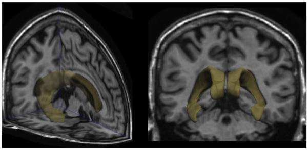
Lateral ventricles in the human brain.
Mathematical preliminaries
Anatomical surfaces in the brain, such as the ventricles, hippocampus, or caudate, have often been analyzed using surface meshes and features derived from them, such as a medial curve, or “skeleton”, that threads down the center of a 3D structure (Thompson et al., 2004). These reference curves are often used to compute the “thickness” of the structure, by assessing the distance from each boundary point to a central line or curve that runs through a structure.
The problem of finding the “medial curve” or “skeleton” of an orientable surface is not well-defined, but a few properties are generally accepted as desirable (Cornea et al., 2005). Here we focus on those properties that are particularly pertinent for registering and comparing surfaces across multiple subjects:
Centered: we would like our curve to be “locally” in the middle of the shape. This is important for accurately estimating local thickness on boundaries of shapes.
Onto, smooth mapping: There must exist a surjective, smooth mapping from the surface to the curve. This is essential in order to use the medial curve for registration.
Consistent geometry: The geometry of the curve should vary smoothly with smooth variations of the shape.
Exploiting the approximately tubular structure of many subcortical regions of interest (ROI), we make the simplifying assumption that our skeleton is a single open curve with no branches or loops. While this is a strong assumption, it greatly simplifies computation, and allows us to focus on (P1) and (P3). In practice, single curve skeletons are robust, even for representing branching shapes like the ventricles (Gutman et al., 2012). Focusing on (P1), we say that a curve is the medial curve if it is smooth and every point on it is “locally in the middle” of the shape. Formalizing this intuition for approximately tubular shapes, we have the following expression for a medial cost function. Given a surface , the medial curve , should be a global minimum of
| (2) |
where c(0),. Here, is the weight defining the “localness” of point p relative to c. Our weight function is defined as in Gutman et al. (2012). Adding a smoothness term penalizing curvature κc, we have our final cost function:
| (3) |
While (P3) is not formally satisfied, it generally holds in practice due to the regularization and the fact that is piecewise smooth. We equip the shapes with two scalar functions for registration based on the medial curve, the global orientation function (GOF) G and medial thickness D:
| (4) |
| (5) |
An example of a medial curve and the corresponding GOF is shown in Fig. 2(A) and the weighting function is illustrated in Fig. 2(B). To ensure (P2), we apply constrained Laplacian smoothing to the GOF if there are any local extrema not at curve endpoints. This step generally requires just a few iterations and is needed in only a small proportion of cases. We modify the framework of Gutman et al. (2012) for longitudinal registration by adding the longitudinal change term:
| (6) |
Fig. 2.
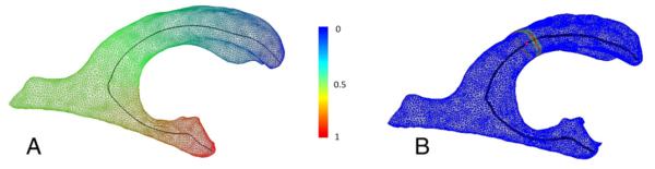
The medial curve of a lateral ventricle surface in one subject from the ADNI cohort. (A) Mesh vertices are colorized by the corresponding Global Orientation Function. (B) Surface weight map from Eq. (2) corresponding to the curve point marked in red. The weight is maximal at the cross-section of the surface with the normal plane of the curve, and decays quickly away from the normal plane.
We first perform longitudinal registration following (Gutman et al., 2012) between each follow-up ventricle model and the corresponding baseline model. Thus, the group-wise registration step of Gutman et al. (2012) is done on only two shapes at a time. We then register each pair of shapes to a corresponding target pair. Unlike Gutman et al. (2012), we do not use group-wise registration during the cross-sectional step to avoid “peaking,” or unfairly biasing our n80 estimate by using information from the testing sample during the learning stage. Instead, we modify the GOF to minimize the L2 difference between the 1D thickness and thickness change maps of the target surface and each new surface, expressed as
| (7) |
where * can correspond to D or ΔD. The 1D registration minimizes
| (8) |
Here the functions f* are the feature functions of each subject’s surface, and g* are the corresponding features of the target shape. The 1D displacement field r is restricted by r:[0,1]→(−1, 1). The GOF is adjusted by Gadj=h−1ºG, h(t)=t–r(t). Surfaces are then registered parametrically on the sphere by simultaneously minimizing the L2 difference between Gadj, D, and ΔD of the new shape and the target shape. The target shape is excluded from LDA training or testing. In this way, each time point and each subject are treated entirely independently; adding new subjects or time points to the dataset does not affect previous results.
LDA-based feature weighting
In designing an imaging biomarker, one generally seeks a balance between the intuitiveness of the biomarker and its power to detect disease or disease progression. A natural choice for ventricular shape-based features is radial expansion. It directly measures anatomical change that correlates with the severity of AD and MCI (Carmichael et al., 2007; Chou et al., 2009; Nestor et al., 2008; Ott et al., 2010; Schott et al., 2010; Thompson et al., 2004; Weiner, 2008). We use the thickness change defined in Eq. (7) as our local measure. Having made this choice, we would now like to find an optimal linear weighting for each vertex on the surface to maximize the effect size of our combined global measure of change. A linear model may not have the intuitive clarity of a binary weighting (i.e., specifying or masking a restricted region to measure), but its meaning is still sufficiently clear and can be easily visualized. Thus we would like to minimize our sample size estimate (1) as a function of the weights, w:
| (9) |
Here C = 32(z1−α/2+Zpower)2, xi is the thickness change for the ith subject, m is the mean vector, the covariance matrix , and SB=mmT. Minimizing Eq. (9) is to maximizing
| (10) |
which is a special case of the LDA cost function, with a maximum given by
| (11) |
For our purposes, m represents the mean of the diseased group. We denote this by m=mAD,MCI, where mAD,MCI stands for the mean expansion vector in the combined MCI and AD group. We make no distinction between these two groups during LDA training. Maximizing (10) directly is generally not stable when SW has a high condition number, as is typically the case when the number of features greatly exceeds the number of examples. For the same reason, even if a stable solution is found, it is unlikely to generalize to a new sample. This is indeed observed for our ventricle data: direct unregularized solutions yield 1-year training n80s between 10 and 30 for MCI subjects, but applying the weighting to a new, non-overlapping sample of MCI data can lead to n80s over 200, comparable to the stat-ROI results. To mitigate this, we use two regularization approaches, one aimed at speed and scalability, and the other at precision and generalizability.
To avoid dealing with dense covariance matrices directly, we apply Principal Components Analysis to our training sample, storing the first k principal components (PCs) in the rows of a matrix, P, and computing the corresponding k eigenvalues λj. This is a standard approach when applying LDA to actual two-class problems, as it makes the mixed covariance matrix nearly diagonal. In our case, the covariance in PCA space is exactly diagonal, which reduces Eq. (11) to a direct computation:
| (12) |
This approach is very fast: one can compute the first k eigenvectors and eigenvalues of SW without explicitly computing SW itself. An alternative to PCA is to incorporate spatial smoothing into Eq. (11) as Tikhonov regularization. This approach is not as efficient as PCA, but allows us to incorporate prior knowledge about the spatial distribution of vertex weights into the solution. Thus it has better potential to generalize across samples. The regularized solution then becomes
| (13) |
Here a is the smoothing weight, and L is the Tikhonov matrix. We use the matrix of surface Laplacian weights between vertices of the average shape computed from healthy controls. To avoid “peaking” with respect to the test n80s for control subjects, a different average shape and Laplacian matrix are computed for each fold during cross-validation. To address the potential lack of disease specificity of ventricular expansion and the power analysis of Eq. (1), we also optimize Eq. (10) for NC-modified sample size estimates. In this case, the mean estimate is modified to
| (14) |
where mNC is the mean expansion among controls.
The order of subjects in each diagnostic group is randomly changed to avoid any confounds such as scanner type, as well as the age or sex of the subject. This step is needed mainly because the standard ADNI subject order corresponds to scanning sites. Where the subjects are scanned is known to correlate with reliability in many morphometric measures. This is only done once before LDA training, with the same order and same subdivision of diagnostic groups used for each method. To validate our data-driven weighting approaches, we create two groups of equal size, with an equal number of MCI, AD and NC subjects in each. Each of these folds is then used to optimize the relevant parameter, i.e., the number of principal components k, the smoothing weight a, or the parametric p-value threshold for stat-ROI. The training fold is again divided into two groups with an equal number of AD and MCI subjects in each, to tune the parameters. The best parameter is then used to train a model on the whole fold, and the model is tested on the other fold. We note that for the PCA approach, a different set of principal components is computed for each fold so that the covariance information from the test set is not used. We further stress that group-wise registration, even if it is blind to diagnosis and time, would constitute a circular analysis here, as the covariance structure of the test set would again be used to inform the training even if indirectly. In fact, the method proposed in Gutman et al. (2012) exploits covariance quite directly. One alternative would be to group-wise register each fold separately. The analysis would even remain objective if we then registered the test fold to a probabilistic atlas created with the training fold, in which case each fold would have two independent homologies, one for testing, and the other for training. However, we did not pursue such complicated schemes, and simply registered all subjects to a single subject template.
A thoughtful reviewer suggested that the two novel aspects of the LDA model compared to the stat-ROI—the continuous weighting, and the multivariate analysis compared to the mass-univariate approach—should be tested separately. In practice, this suggests two additional weightings: a continuous t-statistic weighting, which can be computed directly with no parameter tuning; and a masked version of the LDA. In the latter case, two parameters need to be tuned. In addition to the single parameter already embedded in the model, we also need to find an optimal threshold. For computational speed, we choose to threshold the PCA model. To devise a reasonable set of mask thresholds to test, we compute the cumulative distribution functions (CDFs) of the vertex weights, and space our cutoff values at regular intervals along the y-axis. In other words, each subsequent threshold adds a surface region of a roughly constant area. Further, because the LDA maps are signed, we consider both signed and unsigned masks. For the unsigned case, we use the prior knowledge that ventricles are generally expected to expand, thus considering only positively weighted areas, and weighing the vertices by 1 when the threshold is exceeded. For the signed case, we also assign a value of –1 to vertices whose contraction rate exceeds a threshold. In the latter case, different CDFs and threshold magnitudes are used for the positive and negative regions.
To compute a meaningful anatomical summary from the vertex weights of each weighting scheme, we normalized the weights by their 1-norm, which corresponds to averaging over the ROI for the discrete methods, assuming equal area elements for all vertices. This assumption, however, is only approximately true. These results do not exactly correspond to mean sample sizes reported, since the mean n80 is defined as the average of the two folds’ sample size estimates.
Results
To verify that our measure of annual thickness change has good potential as a biomarker of AD and MCI, we initially performed a group mean comparison of radial thickness change over 1 year using a permutation test as in Thompson et al. (2004). This test relies on the standard t statistic at each vertex, and computes a non-parametric null distribution for the surface area that exceeds the given t-threshold. A threshold corresponding to α<0.05 was used as in Thompson et al. (2004). We compared AD vs. NC groups, and MCI vs. NC. After 100000 random re-assignments of the group data, permutation-based p-values for the overall pattern of group difference for AD vs. NC and MCI vs. NC were below the threshold for each hemisphere, i.e., p<10−5. Localized p-maps of the results are shown in Fig. 3, and are consistent with prior papers by Carmichael et al. (2007), Wang et al. (2011).
Fig. 3.

P-maps show the group differences in annual atrophy rates between healthy controls and (left) AD, and (right) MCI subjects. The progressive expansion from normal aging to MCI/AD is in line with prior reports. Loss of significance near the ends of the medial curve are likely due to the nature of the measurement rather than true anatomical change.
Below we compare the performance of our PCA-based vertex weighting, the Tikhonov-regularized weighting, and the standard stat-ROI approach, as well as t-statistic weighting and signed and unsigned LDA-ROI weightings. In testing each of these weighting methods, we used nested 2-fold cross-validation. Only AD and MCI subjects were used in the training stage. Further, we restricted our training sample to include only 1-year changes. Twenty-four month data was only used for testing, applying 1-year models to the non-overlapping subgroups of the 24-month data.
Our 1-year sample size estimates based on cross-validation were nearly identical for the PCA and the Tikhonov approaches. During training of the PCA model, the optimal number of principal components was chosen to be 28 and 47, for folds 1 and 2, respectively. Maps of the weights averaged over the two folds are shown in Fig. 4A. The Tikhonov approach resulted in predictably smoother weight maps, the mean of which is shown in Fig. 4B. Twenty exponentially increasing values of smoothing weight a were tested, between a=10−2 and a=107. The two folds returned 103.5 and 104 as the optimal values.
Fig. 4.

Continuous weight maps, scaled by standard deviation of the weights. (A) PCA-LDA; (B) Tikhonov-LDA; (C) t-statistic weighting; (D) 2-class PCA-LDA. The weights in (A) and (B) are quite different from the stat-ROI, which indicates that areas of importance in detecting atrophy do not always correspond to the area with highest t-statistic. Compared to (A), (B) shows a similar, but smoother pattern. Most of the area is positively weighted - as expected - though some ventricular contraction is used for a scalar measure as well. This may be partially explained by registration artifact and imprecision in the medial axis, as there is no obvious biological explanation. (D) shows a more disease-specific atrophy pattern. Significantly more weight is given to the inferior horns bordering the hippocampus, and more weighting is also given to the middle of the occipital horns, characteristic of white matter degeneration. Unlike (A)–(C), this map is directly comparable with Fig. 3. The pattern is again different compared to a mass-univariate weighting.
The “stat-ROI” approach led to inferior results with n80s notably higher for all three diagnostic groups, especially MCI. The optimal t-threshold was chosen to be p=10−6 in both folds. The range of tested p-values contained every power of 10 between p=10−4 and p=10−20, which corresponded to ROIs of every size, from patches covering nearly the entire surface (>95%) to just a handful of mesh vertices. The average stat-ROI mask is shown in Fig. 5C. As an additional control, we computed sample size estimates based on ventricular volume change in both hemispheres. Volume-based estimates for the n80 were significantly higher than the three surface-based measures. Table 2 shows a summary of all 1 year sample size estimates. Fig. 6 illustrates the mean sample size estimates for all four measures at 1 year. Bootstrapped 95% confidence intervals (CIs) for each fold were computed as in Schott et al. (2010). To estimate confidence intervals for the whole cohort in an unbiased way, we normalized the linear weights of each fold by their standard deviation. Although the scale of the weighting vector has no bearing on Eq. (1) within each fold, the relative scales of the two vectors can skew the CIs significantly when considered together. Thus, a similar scaling is necessary when computing overall CIs. After this step, the overall CIs were computed the same way as for each fold. We also computed bootstrapped mean n80 comparisons between the different methods for each fold, and for the overall sample. While the two LDA approaches were not significantly different, both led to significantly lower n80s for an MCI clinical trial. The PCA method showed significantly lower estimates for NC subjects, if not corrected for multiple comparisons. P-values for n80 comparisons across the first three methods are summarized in Table 3a.
Fig. 5.

Discrete weight maps. (A) Unsigned LDA-ROI; (B) Signed LDA-ROI; (C) Stat-ROI. Positive ROI is colored in red, negative in blue.
Table 2.
Sample size estimates for clinical trials, using ventricular change over 12 months as an outcome measure. Depending on how we weight the features on the ventricular surfaces, the sample size estimates can be reduced, and the power of the study increased. The two LDA-based methods (top two rows) show lower sample size estimates (i.e., greater effect sizes) than the standard “statistical ROI” approach, which uses a binary mask to select a region of interest. The “t-stat” row shows results when weighting the vertex expansion rates with the t-statistic. “PCA sign.” and “PCA uns.” show results when thresholding PCA-LDA based weight maps, with “sign.” meaning that negatively weighted areas were considered and assigned a weight of −1 when below the threshold. “Uns.” means “unsigned,” i.e. only positively weighted vertices were considered, and weighted with 1 if exceeding the threshold. All surface-based approaches (top six rows) outperform measures of change based on ventricular volume. The “mean” columns display n80s and CIs of the two folds’ estimates averaged. Bold entries represent the lowest point estimates for sample size requirements among the listed methods.
| MCI | AD | NC | Mean MCI | Mean AD | Mean NC | |
|---|---|---|---|---|---|---|
| PCA | 111/96 (85,150)/(75,127) |
65/86 (46,92)/(64,128) |
134/192 (106,177)/(150,260) |
104 (94,139) |
75 (64,102) |
163 (114,190) |
| Tik. | 116/105 (92,154)/(81,146) |
71/95 (49,100)/(65,155) |
155/186 (121,205)/(156,247) |
110 (92,135) |
83 (63,110) |
170 (119,196) |
| Stat-ROI | 184/145 (143,256)/(108,215) |
95/94 (64,143)/(67,143) |
207/201 (159,279)/(155,271) |
165 (134,209) |
94 (72,125) |
204 (156,273) |
| t-stat | 205/151 (154,289)/(112,247) |
91/99 (63,143)/(67,147) |
218/212 (166,298)/(162,288) |
178 (143,232) |
95 (72,128) |
215 (175,264) |
| PCA sign. |
134/111 (104,184)/(83,157) |
85/81 (61,124)/(55,128) |
170/187 (128,242)/(144,251) |
123 (100,154) |
83 (63,111) |
178 (146,222) |
| PCA uns. |
226/161 (166,332)/(120,263) |
95/100 (65,146)/(68,150) |
242/233 (182,339)/(176,323) |
193 (155,261) |
98 (74,130) |
237 (192,296) |
| Vol. | – | – | – | 266 (216,355) |
145 (108,199) |
352 (262,533) |
Fig. 6.
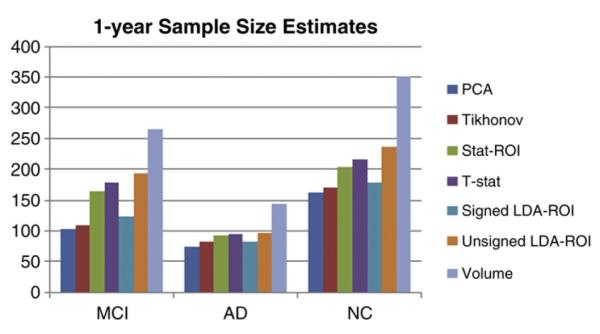
Sample Size Estimates at 1 year. The surface-based estimates are based on nested cross-validation, and averaging the estimates in each non-overlapping fold. PCA and Tikhonov methods require nearly identical samples, while Stat-ROI requires a significantly larger sample of MCI subjects. All surface-based methods need fewer subjects than ventricular volume.
Table 3a.
P-values estimating the evidence that the true 12-month n80 (sample size requirement) of the first method is equal to or greater than that of the second method. Null distributions were created by bootstrapping 100,000 samples with replacement. Note that depending on how rigorous one is about hypothesis testing, the true p-values may need a Bonferroni correction by a factor of 3, if one accepts a separate correction for each subset of the data, or 9 (in which case the two p-values lower than 0.05/9, here, should be considered significant). In either case, n80s for NC subjects are not significantly different among the surface-based methods. At 12 months, the two LDA-based methods give statistically indistinguishable results. P-values below the uncorrected α=0.05 level are shown in bold.
| PCA vs. Tikhonov |
PCA vs. stat-ROI |
Tikhonov vs. stat-ROI |
||||||
|---|---|---|---|---|---|---|---|---|
| MCI | AD | NC | MCI | AD | NC | MCI | AD | NC |
| 0.545 | 0.437 | 0.419 | 0.00475 | 0.200 | 0.0366 | 0.0035 | 0.256 | 0.0529 |
The sample sizes based on t-statistic weighting were very similar to stat-ROI results, with no significant difference, though stat-ROI n80s were generally slightly lower. These weights are visualized in Fig. 4C. The LDA-ROI sample sizes were greater than the continuous weighting, though the difference only reached significance for the unsigned case. For the signed case, 81 and 71 PCs were selected during parameter tuning for the two folds, and the threshold corresponded to 80% of the vertices. For the unsigned case, only 15 and 7 PCs were used, with the threshold set at 90% of the vertices. Comparisons of continuous vs. discrete weightings are presented in Table 3b. The masks resulting from the three discrete methods are visualized in Fig. 5. P-values for n80 comparisons between the discrete and the corresponding continuous weightings are summarized in Table 3b.
Table 3b.
P-values estimating the evidence that the true 12-month n80 (sample size requirement) of the first method is equal to or greater than that of the second method. For LDA, continuous weighting gives better results, but the difference is only significant when using unsigned masking. For stat-ROI, masking is better, but the improvement is not significant. P-values below the uncorrected α=0.05 level are shown in bold.
| PCA vs. signed LDA-ROI |
PCA vs. unsigned LDA-ROI |
Stat-ROI vs. t-stat weighting |
||||||
|---|---|---|---|---|---|---|---|---|
| MCI | AD | NC | MCI | AD | NC | MCI | AD | NC |
| 0.27697 | 0.43547 | 0.27105 | 0.00037 | 0.15134 | 0.00421 | 0.30627 | 0.48339 | 0.35982 |
Finally, the control-augmented sample sizes resulting from the 2-class LDA model resulted in noticeably different maps compared to the 1-class models. We again used the PCA approach, with 32 and 54 principal components used in the two folds. The pattern of the 2-class LDA model was characteristic of AD: significantly more weight was given to the inferior horns bordering the hippocampus, and more weighting was also given to the middle of the occipital horns, characteristic of white matter degeneration. These results are displayed in Fig. 4D. For comparison purposes, we show the control-adjusted sample size estimates for our weightings in Table 4b and Fig. 7B, and also those reported in Holland et al. (2011), in Fig. 9B.
Table 4b.
Sample size estimates for clinical trials, using ventricular change over 24 months as an outcome measure, modified by change in controls. The NC-modified analogues to Table 4a show a marked increase in required sample size. The 2-class model greatly outperforms all other ventricular measures, with ventricular volume performing on par with the best 1-class surface measures: unsigned LDA-ROI and Stat-ROI. Bold entries represent the lowest point estimates for sample size requirements among the listed methods.
| MCI | AD | Mean MCI | Mean AD | |
|---|---|---|---|---|
| PCA | 1170/1373 (659,2758)/(689,4240) |
426/276 (240,1157)/(165,576) |
1272 (760,2239) |
351 (222,610) |
| Tik. | 1661/1595 (859,4892)/(737,6306) |
534/302 (286,1743)/(167,747) |
1628 (902,3440) |
418 (261,875) |
| Stat-ROI | 852/1171 (529,1610)/(623,3171) |
266/241 (169,509)/(150,449) |
1011 (660,1704) |
254 (176,379) |
| t-stat | 840/1298 (517,1628)/(670,3708) |
238/249 (152,433)/(157,459) |
1069 (697,1880) |
244 (171,355) |
| PCA sign. |
1480/1380 (794,3803)/(681,4488) |
482/244 (257,1309)/(140,527) |
1430 (835,2674) |
363 (229,676) |
| PCA uns. |
841/1133 (514,1650)/(611,2958) |
238/233 (150,444)/(147,423) |
987 (641,1696) |
235 (167,357) |
| 2-class |
461/628 (290,841)/(380,1244) |
115/174 (76,191)/(112,306) |
544 (371,802) |
145 (101,192) |
| Vol. | – | – | 916 (658,1385) |
253 (182,372) |
Fig. 7.
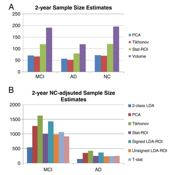
(A) Sample Size Estimates at 2 years. The pattern is similar to estimates at 1 year. The relative difference between stat-ROI and LDA-based methods is greater. (B) NC-adjusted Sample Size Estimates at 2 years. The 2-class model outperforms all other measures. Volume is second best for MCI and on par with the best 1-class measures for AD.
Fig. 9.

(A) Sample size estimates for different ventricular biomarkers. The PCA method is designated here as “Medial Vent-LDA.” The Quarc and Freesurfer measures are for a two-year trial. (B) NC-adjusted Sample size estimates for different ventricular biomarkers. The 2-class PCA method is designated here as “Medial Vent-LDA.” All other results are taken from Holland et al. (2011).
All methods had good agreement between the two folds’ models. The sample sizes in each fold were similar, and the weight patterns were also in good agreement. We used ordinary linear regression for each weighting scheme’s pair of linear models. The null hypothesis that the regression model does not fit the data (F-test) returned p<10−20 for all weighting schemes.
Tables 4a, 4b and 5 show corresponding results for 24-month sample sizes. Here, the general trend is similar to 1-year, though the sample size estimates in controls are closer to estimates for MCI and AD. Fig. 7 illustrates this effect graphically.
Table 4a.
Sample size estimates for clinical trials, using ventricular change over 24 months as an outcome measure. Depending on how the features on the ventricular surfaces are weighted, the sample size estimates can be reduced, and the power of the study increased. The two LDA-based methods (top two rows) show lower sample size estimates than the stat-ROI approach. Control subjects’ average atrophy now approaches that of MCI subjects in magnitude. Bold entries represent the lowest point estimates for sample size requirements among the listed methods.
| MCI | AD | NC | Mean MCI | Mean AD | Mean NC | |
|---|---|---|---|---|---|---|
| PCA | 80/62 (65,108)/(44,86) |
67/47 (47,122)/(31,67) |
69/74 (54,91)/(57,102) |
71 (65,98) |
57 (45,89) |
72 (52,89) |
| Tik. | 73/60 (57,99)/(42,87) |
63/41 (44,117)/(26,63) |
60/80 (47,82)/(62,105) |
67 (54,84) |
52 (38,76) |
70 (48,82) |
| Stat-ROI | 141/96 (113,193)/(69,130) |
93/66 (69,150)/(43,98) |
119/122 (89,177)/(92,182) |
119 (98,149) |
80 (61,108) |
121 (90,179) |
| Vol. | – | – | – | 191 (157,258) |
119 (88,169) |
196 (155,253) |
Table 5.
P-values estimating the chance that the true 24 month n80 of the first method is equal to or greater than that of the second method. Null distributions were created by bootstrapping 100,000 samples with replacement. Note that depending on how rigorous one is about hypothesis testing, the true p-values may need a Bonferroni correction by a factor of 3, if one accepts a separate correction for each subset of the data, or 9. The improvement of the Tikhonov-LDA method over the stat-ROI approach reaches significance, when uncorrected, for AD subjects. At 24 months, the improvement in power when using Tikhonov-regularized LDA model over the PCA model approaches trend levels for MCI subjects. P-values below the uncorrected α=0.05 level are shown in bold.
| Tikhonov vs. PCA |
PCA vs. stat-ROI |
Tikhonov vs. stat-ROI |
||||||
|---|---|---|---|---|---|---|---|---|
| MCI | AD | NC | MCI | AD | NC | MCI | AD | NC |
| 0.129 | 0.257 | 0.334 | 0.00249 | 0.11 | 0.00278 | 0.0001 | 0.0276 | 0.00076 |
To assess whether there is any evidence of longitudinal bias in our weighted measures, we applied our 1 year models to healthy controls at 12 and 24 months. Using a method similar to Hua et al. (2011), we used the y-intercept of the linear regression as a measure of bias (bearing in mind the caveats noted that there may be some biological acceleration or deceleration that could appear to be a bias). We again used bootstrapping to estimate the intercept and linear fit confidence intervals (DiCicio and Efron, 1996). Fig. 8 shows the regression plots for all surface models over the two follow-up time points. Confidence intervals for the linear fits are shown in dotted green lines. The units of change along the y-axis represent the weighted ventricular expansion, normalized by the 1-norm of the weight vectors. The 95% confidence interval for the PCA method was (−0.0218, 0.036) mm, with a mean expansion of 0.111 mm at 1 year and 0.214 mm at 2 years. For the Tikhonov model, the 95% CI was (−0.0126, 0.0242), with mean change at 1 and 2 years of 0.0704 mm and 0.1351 mm, respectively. The stat-ROI summary resulted in a 95% CI of (−0.0411, 0.0645) mm, mean expansion 0.158 mm at 1 year, and 0.306 mm at two years. The bias test results are summarized in Table 6. Group averages for atrophy rates, with each model, are reported in Tables 7a and 7b.
Fig. 8.

Regression plots for surface-based ventricular expansion measures in controls. 95% confidence belts for the regression models are shown with dotted green lines. All surface models are longitudinally unbiased, since the zero intercept is contained in the 95% confidence interval on the intercept, for each of the methods. The 2-class model is trending on additive bias; however, in this model the mean of controls is subtracted for power estimates.
Table 6.
Longitudinal bias analysis of ventricular surface-based measures. Change in healthy controls is linearly regressed over two time points. The intercept is very close to zero, with the confidence interval clearly containing zero for each method. The surface-based measures do not show any algorithmic bias according to the CI test.
| PCA | Tikhonov | T-stat | 2-class LDA |
Signed LDA-ROI | Unsigned LDA-ROI | Stat-ROI |
|---|---|---|---|---|---|---|
| 0.0064 (−0.0218, 0.06) |
0.0048 (−0.0126, 0.0242) |
−0.0102 (−0.0617, 0.0416) |
0.0172 (−0.0031, 0.036) |
−0.0031 (−0.0208, 0.0143) |
−0.0189 (−0.0665, 0.0304) |
0.0115 (−0.0411, 0.0645) |
Table 7a.
Ventricular surface summary atrophy measures for continuous weightings. Averages and standard deviations (in italics) for atrophy rates are in millimeters of radial expansion. The vertex weights are normalized by their 1-norm, which corresponds to averaging over the ROI for the stat-ROI method, assuming equal area elements for all vertices.
| Tikhonov |
PCA |
t-stat |
2-class LDA |
|||||||||
|---|---|---|---|---|---|---|---|---|---|---|---|---|
| MCI | AD | NC | MCI | AD | NC | MCI | AD | NC | MCI | AD | NC | |
| 12 mo | 0.0872±0.060 | 0.105±0.062 | 0.0704±0.054 | 0.151±0.10 | 0.191±0.11 | 0.111±0.084 | 0.247±0.21 | 0.349±0.21 | 0.146±0.14 | 0.058±0.06 | 0.0835±0.073 | 0.0299±0.05 |
| 24 mo | 0.146±0.079 | 0.181±0.086 | 0.135±0.067 | 0.257±0.14 | 0.33±0.17 | 0.214±0.11 | 0.46±0.32 | 0.68±0.37 | 0.304±0.21 | 0.101±0.1 | 0.175±0.13 | 0.0412±0.08 |
Table 7b.
Ventricular surface summary atrophy measures for discrete weightings. Discrete analogues of results in Table 7a, because negative weights are allowed in signed LDA-ROI, the normalized average expansion is closer to the 2-class LDA result, while the unsigned version is closer to stat-ROI and t-statistic weighting. Standard deviations are in italics.
| stat-ROI |
Signed LDA-ROI |
Unsigned LDA-ROI |
|||||||
|---|---|---|---|---|---|---|---|---|---|
| MCI | AD | NC | MCI | AD | NC | MCI | AD | NC | |
| 12 months | 0.262±0.21 | 0.367±0.22 | 0.158±0.14 | 0.0602±0.042 | 0.0796±0.046 | 0.0411±0.035 | 0.226±0.2 | 0.328±0.2 | 0.132±0.13 |
| 24 months | 0.468±0.32 | 0.690±0.39 | 0.306±0.21 | 0.108±0.06 | 0.14±0.068 | 0.083±0.046 | 0.438±0.3 | 0.652±0.36 | 0.284±0.19 |
Discussion
Here we introduced and tested an approach to increase the efficiency of clinical trials in Alzheimer’s disease and MCI, based on multiple neuroimaging features, with a straightforward application of Linear Discriminant Analysis (LDA). We applied our measure of brain change to a surface-based measure of atrophy in the lateral ventricles. Despite the simplicity of our approach, the resulting sample size estimates are significantly better than the stat-ROI approach, which has been the standard feature weighting method to date. The linear feature weighting also produces an intuitive, univariate measure of change—a single number summary that can be correlated to other relevant variables and outcome measures. The linear weights can be easily visualized, adding insight into the pattern and 3D profile of disease progression. Our longitudinal ventricular morphometry showed high sensitivity to local differences in shape change due to AD. Local maps of shape change were consistent with previous studies.
We applied our LDA approach to local ventricular shape change features, with promising results. We used two alternative methods for solving the LDA optimization problem. The first approach, based on principal components analysis, is very fast and scalable to larger feature sets, such as dense Jacobian determinant maps in volumetric Tensor Based Morphometry (TBM). The other optimization method exploits the relatively sparse nature of our surface data by adding Tikhonov regularization in the form of surface-based scalar Laplacian smoothing.
To distinguish between the two novel aspects of the LDA approach with respect to the stat-ROI—multivariate analysis and continuous weighting—we compared three additional weighting schemes. The first is simply the continuous version of the mass-univariate approach used in the stat-ROI, the t-statistic weighting. In cross-validation, this weighting performed slightly worse than the stat-ROI, but the difference did not reach significance. The second and third weighting schemes were designed to be discrete analogues of the PCA-LDA model. These performed worse than the continuous PCA model, with the difference between the unsigned LDA-ROI and the PCA models reaching significance for MCI and NC subjects. However, the signed LDA-ROI model performed notably better than the stat-ROI. These results together suggest that both the continuous and the multivariate aspects of the LDA models contribute to sample size reduction, but the multivariate aspect may play a larger role.
Shape analysis
We have modified a shape registration approach for longitudinal shape analysis in the lateral ventricles. A variety of “medial-curve type” analysis methods for subcortical shapes have been developed over the years. A discrete approach called M-reps was popularized by Pizer et al. (2005) and extended to the continuous setting by Yushkevich et al. (2005). M-reps consist of a discrete web of “atoms,” each of which describes the position, width and local directions to the boundary, and an object angle between corresponding boundary points. The approach leads to an extremely compact representation of the shape model. However, the method requires a specific m-rep model for each type of shape. For a given brain region, this model may need to be modified before it can be applied to a different dataset, if the geometry of the new set of shapes is slightly different, e.g. after being segmented using a different protocol. This drawback is partially overcome when the medial core is continuous.
“CM-reps” are an elegant extension of M-reps to the 2-D continuous medial core. CM-reps offer a way to derive boundaries from skeletons, by solving a Poisson-type partial differential equation with a nonlinear boundary condition (Yushkevich et al., 2005). The resulting 2D medial “sheet” continuously parameterizes the shape-enclosed volumetric region, as well as the surface. Thus in spirit it is very similar to our approach: a particular topology of the continuous medial model is assumed, and the model is deformed to fit each shape. However in certain practical applications, the 2D aspect of the cm-reps model can become a liability, leading to inconsistent parameterization for a family of similar shapes. One such case is the lateral ventricle, where the 2D medial sheet can twist unpredictably around the junction of the superior and occipital horns. Instead, our general approach is to compute a single 1D continuous curve skeleton and use the curve to induce feature functions on the surface. Shape registration is then performed parametrically by minimizing the L2 difference between corresponding feature functions of a pair of shapes. Wang et al. (2011) used radial distance in conjunction with a conformal parameterization and surface-based TBM as an improved measure of ventricular expansion. In this case, a single-curve skeleton was computed based on the conformal parameterization for each ventricular horn. Curve-skeletons of fixed topology have also been used before in medical imaging with distance fields (DFs) (Golland et al., 1999). Our approach avoids the use of DFs, and defines a cost function relating the skeleton directly to the surface, eliminating the imprecision associated with the additional discretization due to DFs. Further, relying only on the discretization of the surface allows us to greatly speed up computation, making analysis of many hundreds of 3D shapes with the continuous medial axis achievable in little time without using large computing clusters.
Machine learning in shape analysis and Alzheimer’s disease
PCA-type approaches have been used in prior shape analyses. A regularized components analysis approach called LoCA (Alcantara et al., 2009) is similar to sparse PCA (Zou et al., 2006). The idea, similar to PCA, is to generate an orthogonal basis for shape space, while adding a penalty term. However, instead of penalizing the number of non-zero weights in each basis vector, as is done in sparse PCA, LoCA instead forces all the non-zero components to be spatially clustered on a surface, which gives each component a clearer anatomical meaning. However, both of these methods come at a much higher computational cost than ordinary PCA: they are iterative, while PCA only relies on eigen-decomposition, making it feasible for much larger feature sets. LoCA has been applied to shape analysis in AD, including ADNI hippocampal data (Carmichael et al., 2012), finding specific component associations with AD and other biomarkers. Here, the measure used was very similar to ours, the radial distance. Only baseline data were used in assessing morphometric differences, while our current study is longitudinal.
Sparse basis decomposition has also been used as a preprocessing step for training an AD classifier, for example by applying Independent Component Analysis (ICA) to gray matter density maps before using machine learning methods, such as Support Vector Machines (SVM), for classification (Yang et al., 2010). Many machine learning approaches have been applied to image-based diagnosis or classification of AD and MCI. Davatzikos and colleagues applied SVM to RAVENS maps (Fan et al., 2008), an approach similar to modified VBM (Good et al., 2002) which assigns relative tissue composition to every voxel after a high-dimensional warp. A similar approach was used by Vemuri et al. (2008), using tissue probability maps (TPMs)—essentially the same VBM measures that are constructed using the SPM package. Kloppel et al. (2008) further showed that such a model can be stable across different datasets. In general, classification algorithms can achieve AD-NC cross-validation accuracy in the mid-nineties (~95%) within the same dataset, although performance inevitably degrades when applied to new datasets, especially if the cohort demographics or scanning protocols are different.
Cuingnet et al. (2010) developed a Laplacian-regularized SVM approach for classifying AD and NC subjects, which is very similar in spirit to our Tikhonov-regularized LDA. They show that using the Laplacian regularizer improves classification rates for AD vs. NC subjects. SVM has also been used, in our prior work, to separate AD and NC subjects based on hippocampal shape invariants and spherical harmonics (Gutman et al., 2009). Another recent surface-based classification effort by Cho et al. (2012) uses an approach very similar to our PCA method, where surface atlas-registered cortical thickness data is smoothed with a low-pass filter of the Laplace-Beltrami operator, computed on the atlas shape. Following this procedure, PCA is performed on the smoothed surface thickness data and LDA is performed on a subset of the PCA coefficients to train a linear classifier. The resulting classification accuracy is very competitive. Another surface-based classifier (Gerardin et al., 2009) uses the SPHARM-PDM approach to classify AD and NC subjects based on hippocampal shape. SPHARM-PDM (Styner et al., 2005) computes a small number of spherical harmonic coefficients based on an area-preserving surface map, and normalizes the spherical correspondence by aligning the first-order ellipsoid with the poles. The result is a rudimentary surface registration and a spectral decomposition of the shape. Gerardin et al. reported competitive classification rates compared to whole-brain approaches. Shen et al. (2010) recently used a Bayesian feature selection approach and classification on cortical thickness data and showed that AD-NC and MCI-NC classification accuracy remains competitive with SVM. Finally, to combine multiple modalities for classification, Zhang et al. (2011) developed a multiple kernel SVM classifier to further improve diagnostic AD and MCI classification.
It is important to stress that while many studies have used machine learning to derive a single measure of “AD-like” morphometry for discriminating AD and MCI subjects from the healthy group, no study we are aware of has used machine learning to maximize the power of absolute atrophy rates in AD. We have attempted this by using a straightforward application of LDA, using either PCA or Tikhonov regularization. The Tikhonov approach was intended to improve generalization relative to PCA, but surprisingly, there were essentially no major differences in test sample size estimates for AD and MCI subjects between the two methods. Only one subgroup at 24 months approached a trend level for a difference in efficiency (sample size difference) between the Tikhonov and PCA model. The Tikhonov method was slightly better for reducing sample size estimates in MCI, generalizing better - as expected. A potential cause of this may be an insufficiently thorough optimal parameter search for the Tikhonov approach, as the search must remain fairly coarse due to computational constraints. On the other hand, it is possible that the covariance structure of the training samples captures the spatial priors sufficiently well, and an explicit prior does not significantly improve generalizability.
Outside of Alzheimer’s literature we found one approach for explicitly minimizing sample size estimates (Qazi et al., 2010), and another that uses SVM for classification of Huntington’s disease patients versus controls, with reduced sample sizes as a by-product (Hobbs et al., 2010). The first paper is methodologically closest in spirit to this work: a fidelity term is explicitly defined to be the control-adjusted sample size estimate. A number of non-linear constraints are then added: the total variation norm (TV1-norm), sparsity and non-negativity. While the first two have analogues that can be linearly optimized as we do here (TV2 and L2 norm), the third constraint forces the authors to use non-linear conjugate gradient (CG), which leads to far slower convergence than the linear CG we use. More importantly, due to the differences in the nature of their data—knee cartilage CT images—and ours, the sparsity and non-negativity constraints are perhaps not appropriate for brain imaging. We expect the effect over soft tissue to be diffuse without many discontinuities, and non-negativity is generally not appropriate in brain MR either. Admittedly, though, as we have focused only on the ventricles, non-negativity would probably be appropriate here, though it would lead to slower convergence. The second paper (Hobbs et al., 2010), which we mention in the introduction, simply uses leave-one-out linear SVM weighting of fluid registration-based TBM maps to derive an atrophy measure. No spatial regularization, or sample size-specific modification to the learning approach is used. In both of these cases the measure used is based on the difference between the mean of controls and the diseased group, which is not the main goal of the present work. Though we have used the NC-adjusted measure here as well to show the potential to reveal AD-specific ventricular change patterns, the main goal was to optimize detection of absolute change.
Other ventricular measures
Several studies have used a ventricular measure alone, as a predictor of cognitive decline. Ott et al. (2010) showed that ventricular volume is associated with CSF Aβ. Carmichael et al. (2007) compared ventricular volume and ventricle–brain ratio (VBR) across MCI converters and non-converters with significantly increased volume, and VBR at baseline among converters. Nestor et al. (2008) used a semi-automated highly precise ventricular segmentation to estimate differences in rates of volumetric change. Rates of volumetric increase in the ventricles were significantly greater in MCI and AD subjects compared to NC, which is in line with expectations about the rates of atrophy in each group. Chou et al. (2009) performed a cross-sectional ventricular study on the baseline ADNI dataset, using a surface-based model. Surfaces were registered—in a similar way to Thompson et al. (2004)—by separating each horn and computing three separate medial axes. The radial distance measure was shown to be significantly different between NC and AD, and NC and MCI subjects. Several other cognitive measures and CSF biomarkers were shown to correlate significantly with the local ventricular surface expansion, in a direction expected from the advancing pathology and the intensification of the disease. Ferrarini et al. (2006) showed differences in local ventricular surface morphometry between AD and NC subjects using permutations testing and a novel algorithm—known as “GAMEs”—for surface meshing and matching.
Power estimates of other measures in AD
Our ventricular change measures outperformed other common ventricular measures as an AD biomarker with respect to the sample size requirements, assuming of course that the reference data are comparable. Schott et al. (2010) reported 1-year n80s for the “Ventricular Boundary Shift Integral” (VBSI) of 118 (92, 157) for AD and 234 (191,295) for MCI at 1 year. Holland et al. (2011) reported a Quarc ventricle measure of 92 (69, 135) for AD and 183 (146, 241) for MCI for a 2-year trial. FreeSurfer ventricular measures give similar 2-year estimates of 90 (68,128) for AD and 164 (133, 211) for MCI. Our approach performs comparably well or better than many other imaging measures, in particular those using the entire cortex. An FSL tool, known as SIENA (Smith et al., 2002; Cover et al., 2011), achieved a 1-year point estimate for sample size of 132 for AD and 278 for MCI. Quarc achieved 2-year whole brain estimates of 84 (63, 123) for AD and 149 (121, 193) for MCI. FreeSurfer is reported (Holland et al., 2011) to achieve 2-year whole brain estimates of 252 (175, 408) for AD and 384 (294, 531) for MCI. Schott reported that BBSI, a whole brain gray matter atrophy measure (Schott et al., 2010), required 1-year samples of 81 (64, 109) for AD and 149 (122, 188) for MCI. Hua et al. (2012) used improved Tensor Based Morphometry (TBM) with the stat-ROI voxel weighting to achieve 1-year sample sizes of 58 (45,81) for AD and 124 (98,160) for MCI. These comparisons are summarized in Figs. 9 and 10. Though all sample size estimates mentioned here are based on the same ADNI-1 dataset, different studies were done on ADNI subsamples of different size. To shed some light on this, we give the number of subjects used for each study in Table 8. Comparison between our study and others is more meaningful where there are fewer exclusions. We note that while the Quarc and Freesurfer results from Holland et al. (2011) are for a 2-year study, and using a slightly different power calculation, in fact even subjects who only had scans up to 1 year were considered. The variance and disease effect in these calculations were based on a mixed effect model using all available time points for each subject. However, there are still roughly 10% fewer subjects used for Quarc and 7% fewer for Freesurfer compared to the full ADNI dataset.
Fig. 10.
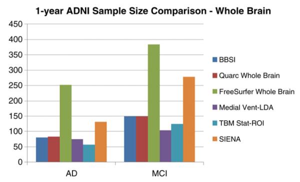
Sample size estimates for different whole biomarkers compared to our ventricular measure. The PCA method applied to ventricular surfaces is designated here as “Medial Vent-LDA.” The Quarc and Freesurfer measures are for a 2-year trial. SIENA estimates are computed from the means and variances reported in Cover et al. (2011).
Table 8.
| AD | MCI | |
|---|---|---|
| Quarc | 131 | 311 |
| FreeSurfer | 135 | 320 |
| BSI | 144 | 334 |
| SIENA | 85 | 195 |
| TBM Stat-ROI | 138 | 326 |
| Medial Vent-LDA | 144 | 337 |
Algorithmic bias
Importantly, we showed that our surface-based measures are longitudinally unbiased according to the intercept CI test (Yushkevich et al., 2010), alleviating common concerns about overly optimistic sample size estimates due to, for example, additive algorithmic bias. The fact that the baseline and follow-up scans were processed identically, and independently, avoids several sources of subtle bias in longitudinal image processing that can arise from not handling the images in a uniform way (Thompson and Holland, 2011). Some issues have been raised regarding the validity of the intercept CI test as a test for bias in estimating rates of change. The CI test assumes that the true morpho-metric change from baseline increases in magnitude linearly over time in healthy controls. Relying on this assumption, the test examines whether the intercept of the linear model, fitted through measures of change at successive time intervals in controls, is zero. If this is not the case, the measure of change is said to have additive bias. There are two common criticisms of this test. First, the linearity assumption may not always be valid, i.e., true biological changes may be nonlinear. In this case, a truly unbiased algorithm could fail the test, while giving accurate results. For example, the loss of tissue may be proportional to the amount of tissue left, so the change in volume as measured by TBM, or medial distance to a ventricular boundary relative to baseline might decay or expand exponentially. Alternatively, if loss of tissue volume is linear in time, radial distance measures might be expected to change in proportion to the cube-root of time, or to vary according to some empirical power law relating the distance to volumetric measures, depending on which directional changes contribute most to the overall change (Zhang and Sejnowski, 2000; Brun et al., 2009). This may partially explain the slight additive “bias” that is detectable in AD and MCI subjects (though not in controls). In disease, the power law describing changes as a function of time may be different compared to controls due to disease effects. As a result, only control subjects should be used when using the linear fit CI test, but even in that case, it is not a perfect test, in that an accurate algorithm could fail the test.
The second common criticism of the CI bias test is that non-additive, atrophy-dependent type of bias may not be detected with the test. In other words, if there exists a complex transfer function between the true change and measured change, a simple linear regression through several time points may not reveal this as a non-zero y-intercept. However, care must be taken when such a transfer function is discovered in an algorithm. It is not simply enough to show the existence of such a function to call an algorithm “biased”; one must also show that the function systematically scales the square of the mean and the variance of the whole sample differently over any number of time points. To address this, we will break the possible transfer functions into four somewhat-overlapping categories, ordered by plausibility, and discuss each. We assume that in all cases an observed transfer function for the mean change is similar in form to the true transfer function for individual subjects.
1. No additive bias and a transfer function whose second derivative has the same sign everywhere
This is perhaps the most likely scenario. For example, measures derived from non-linear deformation fields such as TBM are known to undergo this kind of bias when inverse-consistency is not enforced; page 5 of Tagare et al. (2009) gives a clear explanation for this. In this case, assuming a linear true change, the measured change will follow a non-decreasing (or non-increasing) curve with the same convexity everywhere. Since we assume a zero y-intercept for the curve, a linear fit through two or more time points will inevitably show a non-zero intercept, given enough true change. Thus, the CI intercept test can detect this kind of bias even with just two time points in addition to baseline. Most “known” cases of algorithmic bias that the CI test has so far revealed in literature (Yushkevich et al., 2010; Holland et al., 2011) may well fall in this category.
2. An additive bias and a transfer function whose second derivative has the same sign everywhere
In this case, the additive bias may indeed cancel out the effect of the atrophy-dependent bias, if the second derivative and the additive bias have the same sign. However, this would require quite a special set of circumstances: the sampled time-points and the additive portion of the bias would have to be just right for the linear fit to have a zero y-intercept. With sufficiently many time points, this situation becomes virtually impossible. However, as we have only used three time points, we must admit that this is a possibility, however unlikely, in our study.
3. A strictly linear transfer function with or without additive bias
This scenario is the clearest example of when the CI test would fail. In this case, the measured mean change would be a constant multiple of true mean change. However, it is unclear whether this kind of transfer function can be properly called a “bias.” If such a transfer function had similar form for individual subjects as their sample mean, the sample size estimates would remain unchanged, as the variance would scale in the same way as the square of the mean. On the other hand, it is somewhat difficult to imagine a linear bias that scales the variance and the square of the mean differently for many time points. This would violate our assumption.
4. “Other:” A transfer function with one or more inflection points, with or without additive bias
Though experience with image processing algorithms shows that this scenario is highly improbable, in the interest of completeness we note that this kind of bias can indeed be missed by the CI test, while unfairly inflating power estimates. This is also the only scenario in which our assumption regarding individual bias and bias of the mean will be invalid.
Having gone through this exercise, we hope to have shown that while certain kinds of non-additive bias can potentially be left undetected by the intercept CI test, such a bias is either improbable or does not lead to unfair sample size estimation. Far more likely is the breakdown in the linearity assumption of the CI test, which renders the test inappropriate. Using a subset of the data in which the change is small enough to be at least approximately linear in time, i.e. the control subjects, alleviates the latter issue.
We deliberately chose to use only 12-month data in training our optimized atrophy models. This choice was motivated by practical concerns: we wanted to show that using LDA for optimizing power generalizes sufficiently well to later time points without requiring real drug trials to recompute the atrophy measure for all scans with each new batch of data. This latter situation could be considered a “moving target.” While it may be argued that a better, more parsimonious model could be trained on a sample that includes all available time points, perhaps even incorporating the time variable explicitly, such an approach potentially hides any methodological bias that is inherent in a particular algorithm. Further, a real clinical trial would likely require an ability to apply the same measure to new follow-up scans without requiring one to recompute the measure for all time points every time a new batch of follow-up scans becomes available. In this way, we avoid the moving target problem that bedevils methods requiring scans from all time points. Further, because such methods rely on data-driven techniques to reduce longitudinal bias, for example by computing a per-subject brain atlas based on all available time points, the perceived absence of bias does not indicate that the imaging algorithms themselves are unbiased. This may be called a kind of “peaking” or circularity, as the data used to assess the bias is also used to compute the atrophy measure. However, we do not rely on any data-driven techniques which explicitly force the results to be transitive over time for all available scans. In this sense, the absence of bias in our measures is more indicative of algorithmic objectivity with respect to the amount and direction of morphometric change.
Total and relative atrophy
There has been some recent debate regarding the need to subtract the mean of the healthy controls when estimating sample sizes for a drug trial. Some ADNI collaborators seem to have rejected this idea (Hua et al., 2012; Wyman et al., accepted for publication), in part because real drug trials do not tend to enroll controls, and even if they did, many controls already harbor incipient Alzheimer pathology or some degree of vascular pathology that may also be resisted by treatment. However, the idea is not completely without merit, since all meaningful trials must compare a treatment against another (placebo or established) treatment group. Further, any additive algorithmic bias could be excluded by subtracting the mean rate of controls. In this paper, we addressed this issue by computing an additional linear ventricular expansion model, specific to AD and MCI progression. We did this by directly applying a 2-class, as opposed to 1-class, LDA with the covariance defined strictly by the diseased group, as required by the current practice of NC-adjusted sample size estimates. The resulting power estimates for NC-adjusted atrophy outperform all previous ventricular measures.
Future work
Future work will include combination of multiple biomarkers, including other imaging biomarkers, such as TBM or even non-imaging biomarkers (such as CSF or proteomic measures), into the framework. For example, there is no mathematical reason why only the ventricular measures should be included, as any pertinent structural or functional measure could be incorporated. In the former case, only the PCA-based approach would be feasible due to the high computational cost. It is also important to validate the LDA-weighted measures as well as stat-ROI measures across different data sets. Further, we would like to extend the use of supervised learning to further reduce our sample size estimates. For example, in the PCA experiment, we simply used all principal components—up to a cutoff value. Although the resulting patterns lead to low sample sizes, their spatial distribution contained high-frequency components that may not have anatomical meaning. A more advanced approach would be to perform a greedy boosting-type search over the principal components, with the goal of making the pattern more generalizable and more congruent across the folds. Such a blended LDA-boost approach with built-in cross validation for better fold agreement was proposed in Lu et al. (2003). As our linear weighting is likely to contain a combination of disease effect and systematic registration artifact, a boosting approach over the principal components could potentially isolate and discount any PCs containing the artifactual portion of the variance. Further improvements in sample size estimates could potentially be achieved by modeling out confounding factors such as age and sex, as is done in Schott et al. (2010), and by enrichment techniques that take into account ApoE genotype or family history of AD.
There are two other caveats about comparing n80s that have been raised before. First, basing a measure of brain change on a certain region or parameter of the brain may overlook valuable disease-modifying effects that affect other regions or measures. This is an inevitable consequence when choosing any surrogate outcome measure. Second, the slowing of a change measure by 25% may have different value to the patient, depending on whether the measure is volumetric loss, amyloid clearance, or decline in cognition. As a result, the n80 is a guide to biomarker utility that must be weighed against other relevant criteria, in much the same way as we advocated the weighting of multiple features within an image here, rather than relying on any one marker of disease progression.
Acknowledgments
Data collection and sharing for this project was funded by the Alzheimer’s Disease Neuroimaging Initiative (ADNI) (National Institutes of Health Grant U01 AG024904). ADNI is funded by the National Institute on Aging, the National Institute of Biomedical Imaging and Bioengineering, and through generous contributions from the following: Abbott; Alzheimer’s Association; Alzheimer’s Drug Discovery Foundation; Amorfix Life Sciences Ltd.; AstraZeneca; Bayer HealthCare; BioClinica, Inc.; Biogen Idec Inc.; Bristol-Myers Squibb Company; Eisai Inc.; Elan Pharmaceuticals Inc.; Eli Lilly and Company; F. Hoffmann-La Roche Ltd and its affiliated company Genentech, Inc.; GE Healthcare; Innogenetics, N.V.; IXICO Ltd.; Janssen Alzheimer Immunotherapy Research & Development, LLC.; Johnson & Johnson Pharmaceutical Research & Development LLC.; Medpace, Inc.; Merck & Co., Inc.; Meso Scale Diagnostics, LLC.; Novartis Pharmaceuticals Corporation; Pfizer Inc.; Servier; Synarc Inc.; and Takeda Pharmaceutical Company. The Canadian Institutes of Health Research is providing funds to support ADNI clinical sites in Canada. Private sector contributions are facilitated by the Foundation for the National Institutes of Health (www.fnih.org). The grantee organization is the Northern California Institute for Research and Education, and the study is coordinated by the Alzheimer’s Disease Cooperative Study at the University of California, San Diego. ADNI data are disseminated by the Laboratory for Neuro Imaging at the University of California, Los Angeles. This research was also supported by NIH grants P30 AG010129 and K01 AG030514. Algorithm development for this study was also funded by the NIA, NIBIB, the National Library of Medicine, and the National Center for Research Resources (AG016570, EB01651, LM05639, RR019771 to PT).
Footnotes
Author contributions were as follows: BG and PT wrote the manuscript; BG, XH, PR, YC, AT, and PT performed image analyses; BG, YC, YW, IY, and PT developed algorithms used in the analyses. PT and IY made substantial comments on the manuscript; CJ and MW contributed substantially to the image and data acquisition, study design, quality control, calibration and pre-processing, databasing and image analysis.
References
- Alcantara DA, Carmichael O, Harcourt-Smith W, Sterner K, Frost SR, Dutton R, Thompson P, Delson E, Amenta N. Exploration of shape variation using localized components analysis. IEEE T Pattern Anal. 2009;31:1510–1516. doi: 10.1109/TPAMI.2008.287. [DOI] [PMC free article] [PubMed] [Google Scholar]
- Avants BB, Epstein CL, Grossman M, Gee JC. Symmetric diffeomorphic image registration with cross-correlation: evaluating automated labeling of elderly and neurodegenerative brain. Med. Image Anal. 2008;12:26–41. doi: 10.1016/j.media.2007.06.004. [DOI] [PMC free article] [PubMed] [Google Scholar]
- Beckett LA. Community-based studies of Alzheimer’s disease: statistical challenges in design and analysis. Stat. Med. 2000;19:1469–1480. doi: 10.1002/(sici)1097-0258(20000615/30)19:11/12<1469::aid-sim439>3.0.co;2-j. [DOI] [PubMed] [Google Scholar]
- Brun CC, Lepore N, Luders E, Chou YY, Madsen SK, Toga AW, Thompson PM. Sex differences in brain structure in auditory and cingulate regions. Neuroreport. 2009;20:930–935. doi: 10.1097/wnr.0b013e32832c5e65. [DOI] [PMC free article] [PubMed] [Google Scholar]
- Carmichael OT, Kuller LH, Lopez OL, Thompson PM, Dutton RA, Lu A, Lee SE, Lee JY, Aizenstein HJ, Meltzer CC, Liu Y, Toga AW, Becker JT. Ventricular volume and dementia progression in the Cardiovascular Health Study. Neurobiol. Aging. 2007;28:389–397. doi: 10.1016/j.neurobiolaging.2006.01.006. [DOI] [PMC free article] [PubMed] [Google Scholar]
- Carmichael O, Xie J, Fletcher E, Singh B, DeCarli C. Localized hippocampus measures are associated with Alzheimer pathology and cognition independent of total hippocampal volume. Neurobiology of Aging. 2012;33 doi: 10.1016/j.neurobiolaging.2011.08.016. [DOI] [PMC free article] [PubMed] [Google Scholar]
- Chen K, Langbaum JB, Fleisher AS, Ayutyanont N, Reschke C, Lee W, Liu X, Bandy D, Alexander GE, Thompson PM, Foster NL, Harvey DJ, de Leon MJ, Koeppe RA, Jagust WJ, Weiner MW, Reiman EM. Twelve-month metabolic declines in probable Alzheimer’s disease and amnestic mild cognitive impairment assessed using an empirically pre-defined statistical region-of-interest: findings from the Alzheimer’s Disease Neuroimaging Initiative. Neuroimage. 2010;51:654–664. doi: 10.1016/j.neuroimage.2010.02.064. [DOI] [PMC free article] [PubMed] [Google Scholar]
- Cho Y, Seong JK, Jeong Y, Shin SY. Individual subject classification for Alzheimer’s disease based on incremental learning using a spatial frequency representation of cortical thickness data. Neuroimage. 2012;59:2217–2230. doi: 10.1016/j.neuroimage.2011.09.085. [DOI] [PMC free article] [PubMed] [Google Scholar]
- Chou YY, Lepore N, de Zubicaray GI, Carmichael OT, Becker JT, Toga AW, Thompson PM. Automated ventricular mapping with multi-atlas fluid image alignment reveals genetic effects in Alzheimer’s disease. Neuroimage. 2008;40:615–630. doi: 10.1016/j.neuroimage.2007.11.047. [DOI] [PMC free article] [PubMed] [Google Scholar]
- Chou YY, Lepore N, Avedissian C, Madsen SK, Parikshak N, Hua X, Shaw LM, Trojanowski JQ, Weiner MW, Toga AW, Thompson PM. Mapping correlations between ventricular expansion and CSF amyloid and tau biomarkers in 240 subjects with Alzheimer’s disease, mild cognitive impairment and elderly controls. Neuroimage. 2009;46:394–410. doi: 10.1016/j.neuroimage.2009.02.015. [DOI] [PMC free article] [PubMed] [Google Scholar]
- Cornea ND, Silver D, Yuan XS, Balasubramanian R. Computing hierarchical curve-skeletons of 3D objects. Visual Comput. 2005;21:945–955. [Google Scholar]
- Cover KS, van Schijndel RA, van Dijk BW, Redolfi A, Knol DL, Frisoni GB, Barkhof F, Vrenken H. Assessing the reproducibility of the SienaX and Siena brain atrophy measures using the ADNI back-to-back MP-RAGE MRI scans. Psychiatry Res. 2011;193:182–190. doi: 10.1016/j.pscychresns.2011.02.012. [DOI] [PubMed] [Google Scholar]
- Cuingnet R, Chupin M, Benali H, Colliot O. Spatial prior in SVM-based classification of brain images. Proc SPIE 7624: Medical Imaging 2010: Computer-Aided Diagnosis.2010. p. 7624. [Google Scholar]
- Cummings JL. Integrating ADNI results into Alzheimer’s disease drug development programs. Neurobiol. Aging. 2010;31:1481–1492. doi: 10.1016/j.neurobiolaging.2010.03.016. [DOI] [PMC free article] [PubMed] [Google Scholar]
- DiCicio TJ, Efron B. Bootstrap confidence intervals. Stat. Sci. 1996;11:10. [Google Scholar]
- Duda RO, Hart PE, Stork DG. Pattern classification. Wiley; New York: 2001. [Google Scholar]
- Fan Y, Batmanghelich N, Clark CM, Davatzikos C. Spatial patterns of brain atrophy in MCI patients, identified via high-dimensional pattern classification, predict subsequent cognitive decline. Neuroimage. 2008;39:1731–1743. doi: 10.1016/j.neuroimage.2007.10.031. [DOI] [PMC free article] [PubMed] [Google Scholar]
- Ferrarini L, Palm WM, Olofsen H, van Buchem MA, Reiber JH, Admiraal-Behloul F. Shape differences of the brain ventricles in Alzheimer’s disease. Neuroimage. 2006;32:1060–1069. doi: 10.1016/j.neuroimage.2006.05.048. [DOI] [PubMed] [Google Scholar]
- Fischl B, Dale AM. Measuring the thickness of the human cerebral cortex from magnetic resonance images. Proc. Natl. Acad. Sci. U.S.A. 2000;97:11050–11055. doi: 10.1073/pnas.200033797. [DOI] [PMC free article] [PubMed] [Google Scholar]
- Fox NC, Ridgway GR, Schott JM. Algorithms, atrophy and Alzheimer’s disease: cautionary tales for clinical trials. Neuroimage. 2011;57:15–18. doi: 10.1016/j.neuroimage.2011.01.077. [DOI] [PubMed] [Google Scholar]
- Gerardin E, Chetelat G, Chupin M, Cuingnet R, Desgranges B, Kim HS, Niethammer M, Dubois B, Lehericy S, Garnero L, Eustache F, Colliot O. Multidimensional classification of hippocampal shape features discriminates Alzheimer’s disease and mild cognitive impairment from normal aging. Neuroimage. 2009;47:1476–1486. doi: 10.1016/j.neuroimage.2009.05.036. [DOI] [PMC free article] [PubMed] [Google Scholar]
- Golland P, Grimson WEL, Kikinis R. Statistical shape analysis using fixed topology skeletons: corpus callosum study. Lect. Notes Comput. Sci. 1999;1613:382–387. [Google Scholar]
- Good CD, Scahill RI, Fox NC, Ashburner J, Friston KJ, Chan D, Crum WR, Rossor MN, Frackowiak RS. Automatic differentiation of anatomical patterns in the human brain: validation with studies of degenerative dementias. Neuroimage. 2002;17:29–46. doi: 10.1006/nimg.2002.1202. [DOI] [PubMed] [Google Scholar]
- Gunter J, Bernstein M, Borowski B, Felmlee J, Blezek D, Mallozzi R, Levy J, Schuff N, Jack CR., Jr. Validation testing of the MRI calibration phantom for the Alzheimer’s Disease Neuroimaging Initiative Study. ISMRM 14th Scientific Meeting and Exhibition.2006. [Google Scholar]
- Gutman B, Wang Y, Morra J, Toga AW, Thompson PM. Disease classification with hippocampal shape invariants. Hippocampus. 2009;19:572–578. doi: 10.1002/hipo.20627. [DOI] [PMC free article] [PubMed] [Google Scholar]
- Gutman BA, Yalin W, Rajagopalan P, Toga AW, Thompson PM. Shape matching with medial curves and 1-D group-wise registration. Biomedical Imaging (ISBI), 2012 9th IEEE International Symposium on.2012. pp. 716–719. [Google Scholar]
- Hobbs NZ, Henley SMD, Ridgway GR, Wild EJ, Barker RA, Scahill RI, Barnes J, Fox NC, Tabrizi SJ. The progression of regional atrophy in premanifest and early Huntington’s disease: a longitudinal voxel-based morphometry study. J. Neurol. Neurosurg. Psychiatry. 2010;81:756–763. doi: 10.1136/jnnp.2009.190702. [DOI] [PubMed] [Google Scholar]
- Holland D, Dale AM. Nonlinear registration of longitudinal images and measurement of change in regions of interest. Med. Image Anal. 2011;15:489–497. doi: 10.1016/j.media.2011.02.005. [DOI] [PMC free article] [PubMed] [Google Scholar]
- Holland D, McEvoy LK, Dale AM. Unbiased comparison of sample size estimates from longitudinal structural measures in ADNI. Hum. Brain Mapp. 2012;33:2586–s2602. doi: 10.1002/hbm.21386. [DOI] [PMC free article] [PubMed] [Google Scholar]
- Hua X, Lee S, Yanovsky I, Leow AD, Chou YY, Ho AJ, Gutman B, Toga AW, Jack CR, Jr., Bernstein MA, Reiman EM, Harvey DJ, Kornak J, Schuff N, Alexander GE, Weiner MW, Thompson PM. Optimizing power to track brain degeneration in Alzheimer’s disease and mild cognitive impairment with tensor-based morphometry: an ADNI study of 515 subjects. Neuroimage. 2009;48:668–681. doi: 10.1016/j.neuroimage.2009.07.011. [DOI] [PMC free article] [PubMed] [Google Scholar]
- Hua X, Gutman B, Boyle CP, Rajagopalan P, Leow AD, Yanovsky I, Kumar AR, Toga AW, Jack CR, Jr., Schuff N, Alexander GE, Chen K, Reiman EM, Weiner MW, Thompson PM. Accurate measurement of brain changes in longitudinal MRI scans using tensor-based morphometry. Neuroimage. 2011;57:5–14. doi: 10.1016/j.neuroimage.2011.01.079. [DOI] [PMC free article] [PubMed] [Google Scholar]
- Hua X, Hibar DP, Ching CR, Boyle CP, Rajagopalan P, Gutman BA, Leow AD, Toga AW, Jack CR, Jr., Harvey D, Weiner MW, Thompson PM. Unbiased tensor-based morphometry: improved robustness and sample size estimates for Alzheimer’s disease clinical trials. Neuroimage. 2013;66C:648–661. doi: 10.1016/j.neuroimage.2012.10.086. [DOI] [PMC free article] [PubMed] [Google Scholar]
- Jack CR, Jr., Bernstein MA, Fox NC, Thompson P, Alexander G, Harvey D, Borowski B, Britson PJ, Whitwell JL, Ward C, Dale AM, Felmlee JP, Gunter JL, Hill DL, Killiany R, Schuff N, Fox-Bosetti S, Lin C, Studholme C, DeCarli CS, Krueger G, Ward HA, Metzger GJ, Scott KT, Mallozzi R, Blezek D, Levy J, Debbins JP, Fleisher AS, Albert M, Green R, Bartzokis G, Glover G, Mugler J, Weiner MW. The Alzheimer’s Disease Neuroimaging Initiative (ADNI): MRI methods. J. Magn. Reson. Imaging. 2008;27:685–691. doi: 10.1002/jmri.21049. [DOI] [PMC free article] [PubMed] [Google Scholar]
- Jovicich J, Czanner S, Greve D, Haley E, van der Kouwe A, Gollub R, Kennedy D, Schmitt F, Brown G, Macfall J, Fischl B, Dale A. Reliability in multi-site structural MRI studies: effects of gradient non-linearity correction on phantom and human data. Neuroimage. 2006;30:436–443. doi: 10.1016/j.neuroimage.2005.09.046. [DOI] [PubMed] [Google Scholar]
- Kloppel S, Stonnington CM, Barnes J, Chen F, Chu C, Good CD, Mader I, Mitchell LA, Patel AC, Roberts CC, Fox NC, Jack CR, Jr., Ashburner J, Frackowiak RS. Accuracy of dementia diagnosis: a direct comparison between radiologists and a computerized method. Brain. 2008;131:2969–2974. doi: 10.1093/brain/awn239. [DOI] [PMC free article] [PubMed] [Google Scholar]
- Kloppel S, Abdulkadir A, Jack CR, Jr., Koutsouleris N, Mourao-Miranda J, Vemuri P. Diagnostic neuroimaging across diseases. Neuroimage. 2012;61:457–463. doi: 10.1016/j.neuroimage.2011.11.002. [DOI] [PMC free article] [PubMed] [Google Scholar]
- Kohannim O, Hua X, Hibar DP, Lee S, Chou YY, Toga AW, Jack CR, Jr., Weiner MW, Thompson PM. Boosting power for clinical trials using classifiers based on multiple biomarkers. Neurobiol. Aging. 2010;31:1429–1442. doi: 10.1016/j.neurobiolaging.2010.04.022. [DOI] [PMC free article] [PubMed] [Google Scholar]
- Leow AD, Yanovsky I, Chiang MC, Lee AD, Klunder AD, Lu A, Becker JT, Davis SW, Toga AW, Thompson PM. Statistical properties of Jacobian maps and the realization of unbiased large-deformation nonlinear image registration. IEEE Trans. Med. Imaging. 2007;26:822–832. doi: 10.1109/TMI.2007.892646. [DOI] [PubMed] [Google Scholar]
- Leung KK, Ridgway GR, Ourselin S, Fox NC. Consistent multi-time-point brain atrophy estimation from the boundary shift integral. Neuroimage. 2012;59:3995–4005. doi: 10.1016/j.neuroimage.2011.10.068. [DOI] [PubMed] [Google Scholar]
- Lu J, Plataniotis KN, Venetsanopoulos AN. Boosting linear discriminant analysis for face recognition. ICIP.2003. pp. 657–660. [Google Scholar]
- McKhann G, Drachman D, Folstein M, Katzman R, Price D, Stadlan EM. Clinical diagnosis of Alzheimer’s disease: report of the NINCDS-ADRDA Work Group under the auspices of Department of Health and Human Services Task Force on Alzheimer’s Disease. Neurology. 1984;34:939–944. doi: 10.1212/wnl.34.7.939. [DOI] [PubMed] [Google Scholar]
- Mueller SG, Weiner MW, Thal LJ, Petersen RC, Jack CR, Jagust W, Trojanowski JQ, Toga AW, Beckett L. Ways toward an early diagnosis in Alzheimer’s disease: the Alzheimer’s Disease Neuroimaging Initiative (ADNI) Alzheimers Dement. 2005a;1:55–66. doi: 10.1016/j.jalz.2005.06.003. [DOI] [PMC free article] [PubMed] [Google Scholar]
- Mueller SG, Weiner MW, Thal LJ, Petersen RC, Jack C, Jagust W, Trojanowski JQ, Toga AW, Beckett L. The Alzheimer’s Disease Neuroimaging Initiative. Neuroimaging Clin. N. Am. 2005b;15:869–877. xi–xii. doi: 10.1016/j.nic.2005.09.008. [DOI] [PMC free article] [PubMed] [Google Scholar]
- Nestor SM, Rupsingh R, Borrie M, Smith M, Accomazzi V, Wells JL, Fogarty J, Bartha R. Ventricular enlargement as a possible measure of Alzheimer’s disease progression validated using the Alzheimer’s disease neuroimaging initiative database. Brain. 2008;131:2443–2454. doi: 10.1093/brain/awn146. [DOI] [PMC free article] [PubMed] [Google Scholar]
- Ott BR, Cohen RA, Gongvatana A, Okonkwo OC, Johanson CE, Stopa EG, Donahue JE, Silverberg GD. Brain ventricular volume and cerebrospinal fluid biomarkers of Alzheimer’s disease. J. Alzheimers Dis. 2010;20:647–657. doi: 10.3233/JAD-2010-1406. [DOI] [PMC free article] [PubMed] [Google Scholar]
- Pizer SM, Fletcher PT, Joshi S, Gash AG, Stough J, Thall A, Tracton G, Chaney EL. A method and software for segmentation of anatomic object ensembles by deformable m-reps. Med. Phys. 2005;32:1335–1345. doi: 10.1118/1.1869872. [DOI] [PubMed] [Google Scholar]
- Qazi AA, Jorgensen DR, Lillholm M, Loog M, Nielsen M, Dam EB. A framework for optimizing measurement weight maps to minimize the required sample size. Med. Image Anal. 2010;14:255–264. doi: 10.1016/j.media.2010.01.004. [DOI] [PubMed] [Google Scholar]
- Reuter M, Schmansky NJ, Rosas HD, Fischl B. Within-subject template estimation for unbiased longitudinal image analysis. Neuroimage. 2012;61:1402–1418. doi: 10.1016/j.neuroimage.2012.02.084. [DOI] [PMC free article] [PubMed] [Google Scholar]
- Ross J, Thompson PM, Tariot P, Reiman EM, Schneider L, Frigerio E, Fiorentini F, Giardino L, Calzà L, Norris D, Cicirello H, Casula D, Imbimbo BP. Primary and Secondary Prevention Trials in Subjects at Risk of Developing Alzheimer’s Disease: the GEPARD-AD (Genetically Enriched Population At Risk of Developing Alzheimer’s Disease) Studies. CTAD conference; Monte Carlo, Monaco. 2012. [Google Scholar]
- Schott JM, Bartlett JW, Barnes J, Leung KK, Ourselin S, Fox NC. Reduced sample sizes for atrophy outcomes in Alzheimer’s disease trials: baseline adjustment. Neurobiol. Aging. 2010;31:1452–1462. 1462 e1451–1452. doi: 10.1016/j.neurobiolaging.2010.04.011. [DOI] [PMC free article] [PubMed] [Google Scholar]
- Shen L, Qi Y, Kim S, Nho K, Wan J, Risacher SL, Saykin AJ. Sparse Bayesian learning for identifying imaging biomarkers in AD prediction. Med. Image Comput. Comput. Assist. Interv. 2010;13:611–618. doi: 10.1007/978-3-642-15711-0_76. [DOI] [PMC free article] [PubMed] [Google Scholar]
- Shi Y, Morra JH, Thompson PM, Toga AW. Inverse-consistent surface mapping with Laplace–Beltrami eigen-features. Information Processing in Medical Imaging: Proceedings of the Conference; 2009. pp. 467–478. [DOI] [PMC free article] [PubMed] [Google Scholar]
- Sled JG, Zijdenbos AP, Evans AC. A nonparametric method for automatic correction of intensity nonuniformity in MRI data. IEEE Trans. Med. Imaging. 1998;17:87–97. doi: 10.1109/42.668698. [DOI] [PubMed] [Google Scholar]
- Smith SM, Zhang Y, Jenkinson M, Chen J, Matthews PM, Federico A, De Stefano N. Accurate, robust, and automated longitudinal and cross-sectional brain change analysis. Neuroimage. 2002;17:479–489. doi: 10.1006/nimg.2002.1040. [DOI] [PubMed] [Google Scholar]
- Styner M, Lieberman JA, McClure RK, Weinberger DR, Jones DW, Gerig G. Morphometric analysis of lateral ventricles in schizophrenia and healthy controls regarding genetic and disease-specific factors. Proc. Natl. Acad. Sci. U.S.A. 2005;102:4872–4877. doi: 10.1073/pnas.0501117102. [DOI] [PMC free article] [PubMed] [Google Scholar]
- Tagare HD, Groisser D, Skrinjar O. Symmetric non-rigid registration: a geometric theory and some numerical techniques. J. Math. Imaging Vision. 2009;34:61–88. [Google Scholar]
- Thompson WK, Holland D. Bias in tensor based morphometry Stat-ROI measures may result in unrealistic power estimates. Neuroimage. 2011;57:1–4. doi: 10.1016/j.neuroimage.2010.11.092. [DOI] [PMC free article] [PubMed] [Google Scholar]
- Thompson PM, Hayashi KM, De Zubicaray GI, Janke AL, Rose SE, Semple J, Hong MS, Herman DH, Gravano D, Doddrell DM, Toga AW. Mapping hippocampal and ventricular change in Alzheimer disease. Neuroimage. 2004;22:1754–1766. doi: 10.1016/j.neuroimage.2004.03.040. [DOI] [PubMed] [Google Scholar]
- Vemuri P, Gunter JL, Senjem ML, Whitwell JL, Kantarci K, Knopman DS, Boeve BF, Petersen RC, Jack CR., Jr. Alzheimer’s disease diagnosis in individual subjects using structural MR images: validation studies. Neuroimage. 2008;39:1186–1197. doi: 10.1016/j.neuroimage.2007.09.073. [DOI] [PMC free article] [PubMed] [Google Scholar]
- Wang Y, Song Y, Rajagopalan P, An T, Liu K, Chou YY, Gutman B, Toga AW, Thompson PM. Surface-based TBM boosts power to detect disease effects on the brain: an N=804 ADNI study. Neuroimage. 2011;56:1993–2010. doi: 10.1016/j.neuroimage.2011.03.040. [DOI] [PMC free article] [PubMed] [Google Scholar]
- Weiner MW. Expanding ventricles may detect preclinical Alzheimer disease. Neurology. 2008;70:824–825. doi: 10.1212/01.wnl.0000304743.72127.cc. [DOI] [PMC free article] [PubMed] [Google Scholar]
- Wyman BT, Harvey DJ, Crawford K, Bernstein MA, Carmichael O, Cole PE, Crane P, DeCarli C, Fox NC, Gunter J, Hill D, Killiany R, Pachai C, Schwarz A, Schuff N, Senjem M, Suhy J, Thompson PM, Weiner MW, Jack CR. Standardization of analysis sets for reporting results from ADNI MRI data, Alzheimers Dement. accepted for publication. (epub ahead of print) [DOI] [PMC free article] [PubMed]
- Yang W, Chen X, Hong X, Huang X. ICA-Based Automatic Classification of Magnetic Resonance Images from ADNI Data. Proceedings of the 2010 international conference on Life system modeling and simulation and intelligent computing, and 2010 international conference on Intelligent computing for sustainable energy and environment: Part III.2010. p. 8. [Google Scholar]
- Yuan L, Wang Y, Thompson PM, Narayan VA, Ye J. Multi-source feature learning for joint analysis of incomplete multiple heterogeneous neuroimaging data. Neuroimage. 2012;61:622–632. doi: 10.1016/j.neuroimage.2012.03.059. [DOI] [PMC free article] [PubMed] [Google Scholar]
- Yushkevich PA, Zhang H, Gee JC. Parametric medial shape representation in 3-D via the Poisson partial differential equation with non-linear boundary conditions. Inf. Process. Med. Imaging. 2005;19:162–173. doi: 10.1007/11505730_14. [DOI] [PubMed] [Google Scholar]
- Yushkevich PA, Avants BB, Das SR, Pluta J, Altinay M, Craige C. Bias in estimation of hippocampal atrophy using deformation-based morphometry arises from asymmetric global normalization: an illustration in ADNI 3 T MRI data. Neuroimage. 2010;50:434–445. doi: 10.1016/j.neuroimage.2009.12.007. [DOI] [PMC free article] [PubMed] [Google Scholar]
- Zhang K, Sejnowski TJ. A universal scaling law between gray matter and white matter of cerebral cortex. Proc. Natl. Acad. Sci. U.S.A. 2000;97:5621–5626. doi: 10.1073/pnas.090504197. [DOI] [PMC free article] [PubMed] [Google Scholar]
- Zhang D, Wang Y, Zhou L, Yuan H, Shen D. Multimodal classification of Alzheimer’s disease and mild cognitive impairment. Neuroimage. 2011;55:856–867. doi: 10.1016/j.neuroimage.2011.01.008. [DOI] [PMC free article] [PubMed] [Google Scholar]
- Zou H, Hastie T, Tibshirani R. Sparse principal component analysis. J. Comput. Graph. Stat. 2006;15:265–286. [Google Scholar]