Abstract
Background
Methods using cell line microarray and drug sensitivity data to predict patients’ chemotherapy response are appealing, but groups may be reluctant to release details to preserve intellectual property. Here we describe a case study to validate predictions while treating the methods as a “black box.”
Methods
Medical Prognosis Institute (MPI) constructed cell-line-derived sensitivity scores (SSs) and combined scores (CSs) that incorporate clinical variables. MD Anderson researchers evaluated their predictions. We searched the Gene Expression Omnibus (GEO) to identify validation datasets, and we performed statistical evaluation of the agreement between prediction and clinical observation.
Results
We identified 3 suitable datasets: GSE16446 (n = 120; binary outcome), GSE17920 (n = 130; binary outcome), and GSE10255 (n = 161; continuous and time-to-event outcomes). The SS was statistically significantly associated with primary treatment responses for all studies (GSE16446: P = .02; GSE17920: P = .02; GSE10255: P = .02). Dichotomized SSs performed no better than chance for GSE16446 and GSE17920, and categorized SSs did not predict disease-free survival (GSE10255). SSs sometimes improved on predictions using clinical variables (GSE16446: P = .05; GSE17920: P = .31; GSE10255: P = .045), but gains were limited (95% confidence intervals for GSE16446 and GSE17920 include 0). The CS did not predict treatment response for GSE16446 (P = .55), but it did for GSE17920 (P < .001). Coefficients of clinical variables provided by MPI for CSs agree with estimates for GSE17920 better than estimates for GSE16446.
Conclusions
Model predictions were better than chance in all three datasets. However, these scores added little to existing clinical predictors; statistically significant contributions were likely to be too small to change clinical practice. These findings suggest that discovering better predictors will require both cell line data and a clinical training dataset of patient samples.
A key step in realizing the promise of personalized medicine is to use patients’ genomic profiles and clinical characteristics to predict their response to possible treatments. The first person to develop a practical clinical assay to achieve this goal stands to reap substantial rewards, so there is some incentive to protect intellectual property by presenting the resulting models as “black boxes.” Naturally, evaluating the performance of such black boxes presents considerable challenges.
One particularly appealing approach combines microarray and drug sensitivity data from cell lines to predict chemotherapy response. One high-profile attempt (1–4) had to be retracted (5,6). The Medical Prognosis Institute (MPI) has developed their own method to construct predictive models from cell line data (7). Our research groups agreed to evaluate this method, treating it as a black box. First, the M.D. Anderson authors independently chose datasets satisfying certain conditions (see Methods). The lists of drugs used to treat patients in the chosen datasets were sent to MPI. Second, MPI used their method to develop a predictive model for each drug and sent them back (coded in R). Third, the M.D. Anderson group independently applied the MPI model and compared the predictions to the actual patient outcomes to evaluate the performance. The methods are described, both as an assessment of the MPI models and as an example of how to evaluate black box predictors.
Methods
Dataset Selection
We used two sets of criteria to select datasets. The first set, provided by MPI to ensure the prediction model’s applicability, was as follows:
1. Gene expression profiles should be derived from an Affymetrix Human Genome U133A or U133 Plus 2.0 Array.
2. Let
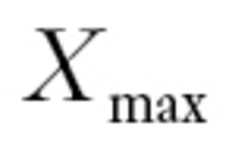 (
(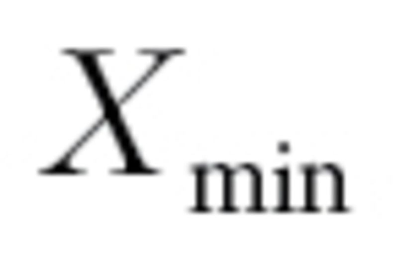 ) denote the largest (smallest) log10 GI50 values for drug X (December 2010; http://dtp.nci.nih.gov/docs/cancer/cancer_data.html). Define
 to be
to be the range of GI50 values. Every drug should have
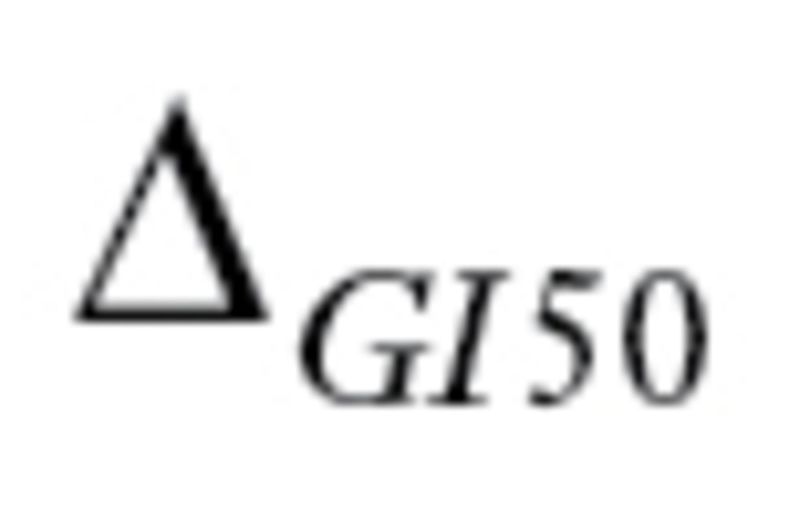 greater than 1 and at least 10 distinct GI50 values. If the National Cancer Institute (NCI) tested drugs using multiple dose ranges, we only used values from the dose range with the most trials.
The second set, determined by M.D. Anderson researchers for model evaluation, was as follows:
3. The dataset should contain at least 100 distinct patients with the same type of cancer.
4. All patients should have received the same treatment.
5. Clinical outcome information that defines treatment success should be available for all patients.
An ideal dataset would meet all criteria, with outcomes blinded to MPI (8). Because such datasets are not available, we chose validation datasets from the public domain. Note, however, that MPI did not use these datasets for model development. We searched GEO (http://www.ncbi.nlm.nih.gov/geo/) and ArrayExpress (http://www.ebi.ac.uk/arrayexpress) to find datasets satisfying the criteria. At GEO, we used the search string “100:10000[NSAM] AND CEL[SFIL] AND GSE[ETYP] AND (GPL96[ACCN] OR GPL570[ACCN] OR GPL571[ACCN] OR GPL1352[ACCN] OR GPL3921[ACCN]).” We manually checked whether the datasets contained at least 100 distinct patients (not arrays), what treatments the patients received, if all drugs met the criteria, and if clinical outcomes were available.
Statistical Analysis
To make predictions, we sent the drug regimens to MPI. They applied methods described previously (7) to GI50 data and to Affymetrix HG-U133A microarray profiles (Genomics Institute of the Novartis Research Foundation, San Diego, CA) from the NCI-60 cell lines to develop predictive models. MPI sent the gene lists and R code specifying their “locked down” model to M.D. Anderson. We independently computed the continuous sensitivity score (SS) using the provided gene list, R code, and Affymetrix data. When clinical information was available, we combined it with the SS using MPI’s predefined coefficients to generate a continuous combined score (CS). Higher scores indicate higher probability of response to therapy.
In one dataset (Hodgkin’s lymphoma; GSE17920), patient samples from different centers exhibited a batch effect (9). We adjusted batch effects using COMBAT (10) and computed SS and CS using both original and batch-corrected gene expression values.
Evaluating Association Between Scores and Outcomes
We used the same procedure, depending on the type of treatment outcome, to evaluate SS and CS.
Binary outcomes.
For binary outcomes, we used receiver operating characteristic (ROC) curves. We calculated areas under ROC curves (AUCs) and 95% confidence intervals (CIs). We used one-sided Wilcoxon rank sum tests to see if the median score was higher in the success group. If the lower bound of the 95% confidence interval of the AUC was less than 0.5, the evaluation ended, and we concluded that the score-based predictions were not better than chance. Otherwise, we performed two further tests. First, to determine if the score added value after adjusting for clinical features, we fit multivariable logistic models. We calculated the scaled Brier score (11,12), and the integrated discrimination improvement (IDI) (13) to compare the clinical model with and without SS. (For CS, we compared the model with only CS to the clinical model.) Second, to assess potential improvement in a clinical setting where decisions are usually based on thresholds, we used cutoffs relevant to the specific disease to dichotomize the continuous scores. We calculated point estimates and 95% confidence intervals for the paired false-positive rate (1 − specificity) and true-positive rate (sensitivity). We also computed point estimates and 95% confidence intervals for the positive predictive value and negative predictive value for the dichotomized scores (14). (For detailed methods and R code, see the Supplementary Methods, available online.) Using the percentile of population treatment failure as the cutoff, we built a reclassification table to compare the predictive performance of SS to predictions made using only clinical features. We computed the corresponding 95% confidence interval for the net reclassification improvement (15). If a standard score [eg, the international prognostic score for Hodgkin’s lymphoma (16)] was available to determine treatment outcome for a specific disease, we compared the performance of SS with this score.
Continuous Outcomes.
For continuous outcomes, we calculated the Spearman rank correlation between SS and treatment outcome. We used the asymptotic t approximation to determine if the rank correlation differed from zero (17). If P was less than .05, the evaluation was completed, and we concluded that the score did not predict patient outcome. Otherwise, we fit multivariable linear models to evaluate whether SS added value after adjusting for clinical features.
Right-Censored Treatment Outcomes.
For time-to-event outcomes, we fit Cox regression models using SS as the predictor. If P was less than .05, the evaluation was completed, and we concluded that SS did not predict survival. Otherwise, we fit multivariable Cox models to evaluate whether SS statistically significantly added value after adjusting for clinical features.
Evaluating the Combined Score
The CS from MPI incorporates age and stage with the same coefficients for every type of cancer and thus assumes that these features contribute to every response in the same way. In contrast, we fit multivariable models to estimate effects of age and stage in each study.
We performed all analyses using the R statistical software environment, version 2.15.1 (R Foundation for Statistical Computing, Vienna, Austria). The gene lists, R code to generate sensitivity scores, and complete documentation underlying our results are available at http://bioinformatics.mdanderson.org/Supplements/MPI.
Results
Dataset Searching
Using the search string (see Methods) in GEO in December 2010 yielded 203 studies that contained at least 100 microarray “cel” files from either Affymetrix Human Genome U133A or U133 Plus 2.0 Arrays. A list of all 203 studies is provided in Supplementary Table 1 (available online).
In GEO, one dataset is sometimes a subset of another; in this case, we only retained the larger dataset. Manually eliminating subsets reduced the 203 datasets to 191. Of these, 102 (54%) contained gene expression profiles from patient tumor samples. The others included samples from healthy people or cell lines. Of the 102 tumor datasets, 74 (73%) contained data from at least 100 distinct patients. Only 39 of 74 (53%) contained clinical information giving the individual treatment outcome for each patient, and only 24 of 74 (31%) specified the treatment that each individual patient received. In total, only 23 datasets in GEO meet criteria 3 through 5 for model validation purposes. A similar investigation in ArrayExpress yielded zero datasets satisfying these criteria. Detailed information about these 23 datasets is given in Supplementary Table 2 (available online).
Next, we checked whether the 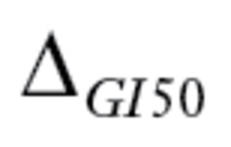 values for the drug regimens used to treat patients in the 23 datasets satisfied criteria 1 and 2 defined by MPI. The
  values for drugs commonly used in cancer treatments are summarized in Supplementary Table 3 (available online). Many drugs commonly used in cancer therapy (eg, cyclophosphamide, tamoxifen) do not meet the criteria. In total, only three datasets (GSE16446, GSE17920, and GSE10255) satisfied all five criteria. Moreover, when we contacted the authors of GSE10255 to obtain the clinical data, we learned that the initial publication (18) describing the GSE10255 dataset used an additional independent set of 92 patients that is not available in GEO. These 92 patients were treated the same as the patients in GSE10255, and disease-free survival (DFS) times were available. Hence, we obtained the DFS data, Affymetrix U133A data, and clinical covariables for these patients from the authors at St. Jude under a material transfer agreement and included these in our study.
Evaluation Results for GSE16446 (Breast Cancer)
The first dataset was GSE16446 (19,20) from a study of 120 breast cancer patients treated with epirubicin monotherapy, which satisfies the drug regimen criteria ( ). The primary endpoint was a binary outcome, pathological complete response. MPI provided both SS and CS; we present results for each.
The SS AUC was statistically significant; adding the SS to clinical features gave limited improvement; the dichotomized SS was not better than chance. Figure 1A for study GSE16446 shows that the SS has an AUC statistically significantly greater than 0.5 (AUC = 0.65, 95% CI = 0.52 to 0.79; P = .02). Multivariable logistic regression suggests modest additional predictive ability of the SS after adjusting for clinical features (estimated coefficient = 0.03; P = .05). Comparing the overall performance of the clinical model with and without the SS, prediction accuracy improved when the SS was added; the scaled Brier score increased from 0.01 to 0.06 (Table 1). However, the improvement was limited. The 95% confidence intervals for the AUCs overlap for the models with the SS (0.53 to 0.82) and without SS (0.44 to 0.74). The IDI is not substantially greater than zero (IDI = 0.168, 95% CI = −0.12 to 0.46) (Table 1).
Figure 1.
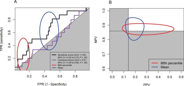
Receiver operating characteristic (ROC) curves of combined score and sensitivity score to predict pathological complete response and 95% confidence intervals of paired (false-positive rate [FPR], true-positive rate [TPR]) and (positive predictive value [PPV], negative predictive value [NPV]) for sensitivity score with two different cutoff points for study GSE16446 (breast cancer). A) Ninety-five percent confidence intervals for (FPR, TPR) sensitivity score. The solid black line and orange line are the ROC curves for sensitivity score and combined score, respectively. B) Ninety-five percent confidence intervals for (PPV, NPV) sensitivity score. Cutoff points were 1) the 86th percentile (1 − the pathological complete response rate of GSE16446 study; red ellipses) and 2) the mean (the standard cutoff point used by the Medical Prognosis Institute; blue ellipses). Gray area indicates the region for the prediction made by chance. AUC = area under the curve; CI = confidence interval.
Table 1.
Performance of the clinical features (age and stage) with or without sensitivity score, and combined score to predict treatment outcome for study GSE16446 (breast cancer)*
| Model | Brier scaled | AUC (95% CI) | IDI (95% CI) |
|---|---|---|---|
| Grade + size + age | 0.01 | 0.59 (0.44 to 0.74) | Baseline model |
| Grade + size + age + sensitivity score | 0.06 | 0.67 (0.53 to 0.82) | 0.168 (−0.12 to 0.46) |
* AUC = area under the curve; CI = confidence interval; IDI = integrated discrimination improvement.
Because the SS was statistically significant in both univariable and multivariable analyses, we checked to see if it was likely to prove useful in a clinical setting where test results are often dichotomized. We used two reasonable cutoffs: 1) the 86th percentile of all scores, which is the rate of pathological complete response for the patients in GSE16446; and 2) the mean of all combined scores. We summarized the point estimates for true-positive rate, false-positive rate and (positive predictive value, negative predictive value in Supplementary Table 4 (available online); we plotted their 95% confidence intervals in Figure 1. At the specified cutoffs, the prediction models using the SS alone did not perform better than chance. In addition, using the 86th percentile as the cutoff, 16 patients (of 109 for whom clinical covariables were available) were reclassified, but the net reclassification improvement was not greater than zero (Table 2) (net reclassification improvement = 0.17, 95% CI = −0.13 to 0.47).
Table 2.
Reclassification table for the prediction performance without and with the sensitivity score for study GSE16446 (breast cancer)*
| Grade + size + age | Grade + size + age + sensitivity score (NRI = 0.17; 95% CI = −0.13 to 0.47) | Total | |
|---|---|---|---|
| Not pCR | pCR | ||
| Not pCR | 88 (10 pCR) | 11 (4 pCR) | 99 (14 pCR) |
| pCR | 5 (1 pCR) | 5 (0 pCR) | 10 (1 pCR) |
| Total | 93 (11 pCR) | 16 (4 pCR) | 109 (15 pCR) |
* Cutoff point = 86th percentile (1 − pathologically complete response rate of GSE16446 study). CI = confidence interval; NRI = net reclassification improvement; pCR = pathologically complete response.
The CS did not show statistically significant differences between pathological complete response and non–pathological complete response patients. The P value of the one-sided Wilcoxon test was .55, and the ROC curve is plotted in Figure 1A. The corresponding AUC is 0.51 (95% CI = 0.36 to 0.66).
Evaluation Results for GSE17920 (Hodgkin Lymphoma)
The second dataset, GSE17920 (9), included 130 patients with Hodgkin lymphoma who received a standard treatment called ABVD, which is a combination of four drugs: doxorubicin (adriamycin, ), bleomycin (
 ), vinblastine (
 ), and dacarbazine (
 ). All drugs satisfy the criteria defined by MPI. The primary endpoint was a binary variable indicating treatment success or failure.
The 130 tumor samples came from two sources: 100 from Vancouver and 30 from Nebraska. Treatment outcomes differ by source, with 82 of 100 successes in Vancouver and 10 of 30 in Nebraska (P < .0001) (Supplementary Table 6, available online). To measure the impact of batch effects on prediction, we computed the SS and CS using both the original gene expression values and the gene expression values adjusted for batch effects.
The SS AUC was statistically significant but equivalent to the International Prognostic Score (IPS) AUC; adding the SS to clinical features gave no improvement; the dichotomized SS was not better than chance. The ROC curves for both the original and adjusted SS are plotted in Supplementary Figure 1A (available online) (AUC = 0.62, 95% CI = 0.52 to 0.72 using the original gene expression values). The AUC was statistically significantly greater than 0.5 on the full data set (P = .02) and on the larger Vancouver subset (P = .02). It was not statistically significant on the Nebraska subset (Table 3). IPS is an existing clinical model, defined as the number of adverse prognostic factors present at diagnosis (16), which ranges from 0 to 7. Higher IPS indicates lower probability of a successful outcome. The ROC curve for IPS was plotted in Supplementary Figure 1A (available online); the AUC was also 0.62 (95% CI = 0.52 to 0.72). Hence, the SS AUC was not statistically significantly different from the IPS AUC.
Table 3.
P values of one-dided Wilcoxon rank sum test for different scores by treatment success and treatment failure group in study GSE17920 (Hodgkin’s lymphoma)*
| Variable | Based on original GE | Based on adjusted GE | ||||
|---|---|---|---|---|---|---|
| All | Vancouver | Nebraska | All | Vancouver | Nebraska | |
| Combined score | .0001 | .0008 | .59 | .0004 | .0008 | .61 |
| Sensitivity score | .02 | .02 | .95 | .06 | .02 | .95 |
* All indicates 130 patient samples from both Vancouver center and Nebraska center. Vancouver indicates 100 Vancouver patient samples only. Nebraska indicates 30 Nebraska patient samples only. GE = gene expression.
Multivariable logistic regression suggested no additional predictive ability of the SS after adjusting for patient clinical features (P = .31). Comparing the overall prediction performance of the clinical model with and without SS, the scaled Brier score stayed the same (Table 4). The improvement in prediction was not statistically significant. Neither the AUC changes nor the IDI were greater than zero (Table 4).
Table 4.
Performance of the clinical features (age and stage) with or without sensitivity score, and combined score to predict treatment outcome for study GSE17920 (Hodgkin’s lymphoma)*
| Model | Brier scaled | AUC (95% CI) | IDI (95% CI) |
|---|---|---|---|
| Age + stage | 0.11 | 0.68 (0.57 to 0.79) | Baseline model |
| Age + stage + sensitivity score (original) | 0.12 | 0.70 (0.60 to 0.81) | −0.04 (−0.10 to 0.03) |
| Age + stage + sensitivity score (adjusted) | 0.11 | 0.68 (0.58 to 0.80) | −0.04 (−0.11 to 0.03) |
| Combined score (original) | 0.11 | 0.70 (0.60 to 0.80) | −0.04 (−0.19 to 0.12) |
| Combined score (adjusted) | 0.10 | 0.68 (0.58 to 0.79) | −0.04 (−0.15 to 0.08) |
* AUC = area under the curve; CI = confidence interval.
The CS AUC was statistically significant but equivalent to the IPS AUC; the dichotomized CS predicted response; the dichotomized CS performed equivalently to the model with only clinical features and to the IPS. We performed one-sided Wilcoxon rank sum tests for the CS generated from the prediction models using both original and adjusted gene expression values. The CS based on the original gene expression values were statistically significantly higher in the treatment success than in the treatment failure group (P = .0001 for all samples; and P = .0008 for Vancouver samples) (Table 3). Similarly, CS based on adjusted gene expression values were statistically significantly higher in the treatment success than in the treatment failure group (P = .0004 all samples; and P = .0008 for Vancouver samples) (Table 3). The ROC curves for the CS are plotted in Supplementary Figure 1C (available online) (original score AUC = 0.70, 95% CI = 0.60 to 0.80; adjusted score AUC = 0.68, 95% CI = 0.58 to 0.79). This figure and the Wilcoxon test results above show that the AUC for the CS is statistically significantly greater than 0.5; however, the CS AUC was still not statistically significantly greater than the IPS AUC (AUC = 0.62, 95% CI = 0.52 to 0.73).
The scaled Brier score for the logistic model with the CS alone was 0.11 for the original score and 0.10 for the adjusted score. These were less than (or equal to) the scaled Brier score for the logistic model with only clinical features (Table 4). Similarly, the AUC and IDI did not show any improvement for the model with the CS alone compared with the model using only clinical features.
Evaluation Results for GSE10255 (Acute Lymphoblastic Leukemia)
The last dataset that we evaluated came from a study of gene expression in primary acute lymphoblastic leukemia (ALL) associated with methotrexate (MTX) treatment response (18). The patients were randomized to receive one of three treatments: 1) high-dose MTX by infusion over 4 hours (n = 70); 2) high-dose MTX by infusion over 24 hours (n = 74); or 3) high-dose MTX by infusion over 24 hours plus mercaptopurine (MP) (n = 17). The primary endpoint was the difference, 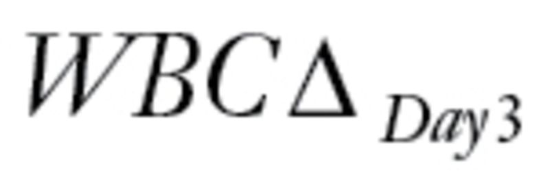 , between levels of circulating leukemia cells measured before therapy (WBCPRE) and at day 3 after the start of a treatment (WBCDay3).
  was determined by taking the residuals of a linear regression model of log(WBCDay3) versus log(WBCPRE ).
 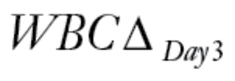 is an important predictor of survival for ALL; lower levels predict longer survival. Even though the patients were treated with three different protocols, because a single dose of intravenous MP has little antileukemic effect (21), and because WBCPRE and WBCDay3 are similar (P > .13) among the treatment groups (18), we ignored the treatment difference and viewed all patients as having received the same treatment.
GSE10255 contains Affymetrix gene expression data on 161 patients. We obtained clinical data including sex, age at diagnosis, and ALL subtype from St. Jude Children’s Research Hospital. MPI provided the information to derive the SS (but not the CS) for each patient. To study DFS, we used an independent set of 92 patients obtained directly from St. Jude (see the details in the “Dataset Searching” subsection).
SS was a statistically significant predictor for WBCΔDay3 with and without adjusting for clinical features for the dataset with 161 patients. The Spearman correlation between SS and WBCΔDay3 was −0.18 (P = .02). A scatter plot for the two variables is presented in Figure 2A. Multivariable regression showed that after adjusting for sex, patient age, WBCPRE, and ALL subtypes, the SS remained a statistically significant predictor for WBCΔDay3 (P = .045) (Table 5), although the reclassification index did not show substantial improvement (Supplementary Table 7, available online).
Figure 2.
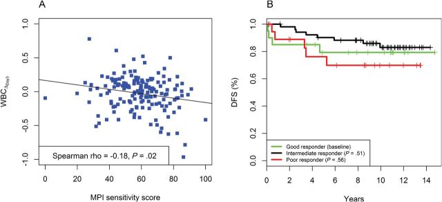
Association between the Medical Prognostic Institute (MPI) sensitifit score and outcome in study GSE10255 (acute lymphoblastic leukemia). A) Scatter plot of sensitivity score versus change in the levels of circulating leukemia cells at day 3 after the start of treatment ( ) and the fitted line by linear regression. B) Kaplan-Meier plots of disease-free survival (DFS) categorized by MPI sensitivity score. A good responder was a patient with top 25% sensitivity scores (n = 20). An intermediate responder was a atient with middle 50% sensitivity scores (n = 53). A poor responder was a patient with bottom 25% sensitivity scores (n = 19).
Table 5.
Multivariable linear regression of Medical Prognosis Institute sensitivity score related to change in the levels of circulating leukemia cells at day 3 after the start of treatment adjusting for the clinical prognostic factors for study GSE10255 (acute lymphoblastic leukemia). All subtypes are as defined by Sorich and colleagues (18).
| Parameter | Estimate | Standard error | P |
|---|---|---|---|
| Sensitivity score | −0.003 | 0.001 | .045 |
| Sex: male vs female | −0.044 | 0.042 | .30 |
| Age: ≥10 y vs <10 y | −0.005 | 0.054 | .93 |
| log(WBCPRE) | −0.013 | 0.035 | .71 |
| Subtype | |||
| BCR-ABL vs B other | 0.277 | 0.135 | .04 |
| E2A-PBX1 vs B other | −0.019 | 0.077 | .80 |
| Hyperdiploid vs B other | 0.032 | 0.058 | .59 |
| MLL-AF4 vs B other | −0.078 | 0.184 | .67 |
| T-lineage vs B other | −0.012 | 0.072 | .52 |
| TEL-AML1 vs B other | −0.019 | 0.064 | .77 |
Neither the continuous nor categorized SS predicted DFS with or without adjusting for clinical features for the dataset with 92 patients. A univariable Cox model showed that the continuous SS was not a statistically significant predictor for DFS (Supplementary Table 8, available online). Following the procedures used by Sorich et al. for their predictions (18), we trichotomized the continuous SS using the 25th and 75th percentiles as cutoffs. Patients in the top quartile were defined as good responders, and patients in the bottom quartile were defined as poor responders. All other patients were defined as intermediate responders. A Cox model showed that this categorized score was still not a statistically significant predictor of DFS.
Different Clinical Scores for Different Diseases
We used stepwise backward model selection to estimate linear coefficients to combine the SS with clinical characteristics (Table 6). Compared with the “absolute” coefficients provided by MPI, the estimated coefficients were similar in study GSE17920 but different in study GSE16446. This observation may explain why the CS for study GSE16446 had a poor predictive ability.
Table 6.
Comparison of coefficients of sensitivity score and clinical features from multivariable logistic model and coefficients provided by the Medical Prognostic Institute (MPI)*
| Variable | GSE16446 (breast cancer) | GSE17920 (Hodgkin’s lymphoma) | ||
|---|---|---|---|---|
| Multivariable model | MPI model | Multivariable model | MPI model | |
| Sensitivity score | 0.03 (.05) | 1 | 0.01 (.31) | 1 |
| Age, continuous | — | -— | −0.02 (.11) | −1 |
| Aged ≥50 or not | 0.52 (.37) | −50 | -— | -— |
| Stage | -— | -— | −0.59 (.01) | -25 |
| Grade | 0.30 (.65) | 30 | -— | -— |
| Size | 0.28 (.38) | −25 | -— | -— |
* If the predictor is not in the final logistic model, the coefficient for that predictor is considered to be zero. The value in parentheses is the P value for the predictor.
Discussion
We set out to clarify whether the SS and CS proposed by MPI could predict patient response. We conclude that the method proposed by MPI to use cell lines to develop predictive models yields predictions in patient samples that are better than chance, but the predictions are not yet good enough to change clinical practice. The SS predictions were statistically significant (as measured by Wilcoxon test or AUC) in all three cases that we examined. In two of three cases, SS even added value beyond using clinical variables (GSE16446: P = .05; GSE17920: P = .31; GSE10255: P = .045). However, when we tried to quantify the gain using the scaled Brier score, IDI, or reclassification tables, the improvement was negligible or nonexistent. The fact that there was a gain suggests that a refinement of the MPI procedure might be able to improve predictions of response.
However, trying to develop models from cell lines alone is likely to be only one step toward the goal of making better predictions. For instance, we found that there was a large difference between MPI’s proposed clinical coefficients for the CS and the coefficients from the logistic model learned directly from dataset GSE16446, breast cancer treated neoadjuvantly with epirubicin. It was probably a mistake to include the clinical variable age in the combined score to begin with because there is no evidence that it is correlated to pathological complete response in neoadjuvant treatment of breast cancer (22). Prediction of response to treatment in metastatic breast cancer, a focus of much new drug development, may present a significant opportunity for the in vitro–based models presented here because no established clinical variables predict treatment response in this clinical setting except for biomarkers such as estrogen receptor, progesterone receptor, and human epidermal growth factor receptor 2. In either the primary tumor or metastatic setting, further development of predictive models is likely to require input from clinical oncologists about the clinical variables to include, along with a training dataset consisting of actual patient samples to calibrate the models.
The drug regimen criteria proposed by MPI provide some idea of when the approach of using cell line chemosensitivity to predict treatment should be attempted. However, the criteria may be too strict in that some commonly used cancer drugs, such as cyclophosphamide and tamoxifen, do not meet the criteria. To solve the problem of predicting treatment response involving drugs that fail to meet the drug criteria, MPI is working on a prediction model based on the same underlying approach but using other sources with more cell line information [eg, Cancer Cell Line Encyclopedia (23)] for assessing relative sensitivity scores for treatments involving cyclophosphamide. Moreover, because the Cancer Cell Line Encyclopedia contains measurements of multiple genomics features (gene expression, chromosomal copy number, and massively parallel sequencing data) on the same cell lines (23), one might be able to develop integrated models with greater power to predict drug sensitivity.
The idea of using cell line chemosensitivity to predict patient response to cancer therapeutics is appealing. However, poor documentation and erroneous results in the initial reports led to the approach being greatly oversold. Here, we tried to make a more realistic assessment by evaluating a modeling approach proposed by MPI. Our evaluation method represents a compromise between the need for complete specification of an analysis and the need to protect intellectual property. [In previous recommendations (24, 25), we anticipated the need to compromise between complete disclosure of methods and the requirement to protect intellectual property.] The M.D. Anderson team did not know the full details of how the models were constructed. However, we chose the datasets used for validation, and we insisted that the final models be supplied in “locked down” form with rules specifying exactly what gene values should be combined and how to produce a score.
In this article, we also discussed the basic steps we took to evaluate the prediction model. These steps can easily be generalized to evaluate any black box models that apply microarray or other studies to enhance personalized medicine and patient care. In the future, we expect more studies will be performed to propose or validate such models. However, there are some limitations for researchers using publicly available datasets to perform these kinds of studies.
Expression profiles of patients are relatively easy to access today because of widespread acceptance of the Minimum Information About a Microarray Experiment (MIAME) standard (26). Clinical information, however, especially patient treatment and response information vital to these kinds of studies, is still difficult to obtain. We initially expected that far more than three datasets would meet our criteria. Because publishing clinical data or relevant metadata along with the expression profiles is not mandatory, many researchers publish part or none of their clinical data. Sometimes, the clinical data are available as supplementary material, but most of the time, there are no detailed clinical data publicly available beyond summary tables of patient characteristics. We encourage researchers to submit the relevant clinical information along with the microarray datasets to the online data archives. Elsewhere, we have suggested extensions to the XML format used by GEO to store microarray data to make it easier to accommodate structured clinical data (25), In the meantime, the automatic filters at the online data archives also need to be modified to accommodate these clinical characteristics for easier searching purposes.
Funding
SK, WM, and JA received support from the Danish Council for Strategic Research. WW, KRC, and KAB received support from MPI.
Supplementary Material
We thank St. Jude’s Children’s Hospital for supplying additional data.
References
- 1. Augustine CK, Yoo JS, Potti A, et al. Genomic and molecular profiling predicts response to temozolomide in melanoma. Clin Cancer Res. 2009;15(2):502–510 [DOI] [PubMed] [Google Scholar]
- 2. Bonnefoi H, Potti A, Delorenzi M, et al. Validation of gene signatures that predict the response of breast cancer to neoadjuvant chemotherapy: a substudy of the EORTC 10994/BIG 00-01 clinical trial. Lancet Oncol. 2007;8(12):1071–1078 [DOI] [PubMed] [Google Scholar]
- 3. Hsu DS, Balakumaran BS, Acharya CR, et al. Pharmacogenomic strategies provide a rational approach to the treatment of cisplatin-resistant patients with advanced cancer. J Clin Oncol. 2007;25(28):4350–4357 [DOI] [PubMed] [Google Scholar]
- 4. Potti A, Dressman HK, Bild A, et al. Genomic signatures to guide the use of chemotherapeutics. Nat Med. 2006;12(11):1294–1300 [DOI] [PubMed] [Google Scholar]
- 5. Baggerly KA, Coombes KR. Deriving chemosensitivity from cell lines: forensic bioinformatics and reproducible research in high-throughput biology. Ann Appl Stat. 2009;3(4):1309–1334 [Google Scholar]
- 6. Coombes KR, Wang J, Baggerly KA. Microarrays: retracing steps. Nat Med. 2007;13(11):1276–1277; author reply 1277–1278 [DOI] [PubMed] [Google Scholar]
- 7. Chen JJ, Knudsen S, Mazin W, Dahlgaard J, Zhang B. A 71-gene signature of TRAIL sensitivity in cancer cells. Mol Cancer Ther. 2012;11(1):34–44 [DOI] [PubMed] [Google Scholar]
- 8. Institute of Medicine Evolution of Translational Omics: Lessons Learned and the Path Forward. Washington, DC: National Academies Press; 2012. [PubMed] [Google Scholar]
- 9. Steidl C, Lee T, Shah SP, et al. Tumor-associated macrophages and survival in classic Hodgkin’s lymphoma. N Engl J Med. 11 2010;362(10):875–885 [DOI] [PMC free article] [PubMed] [Google Scholar]
- 10. Johnson WE, Li C, Rabinovic A. Adjusting batch effects in microarray expression data using empirical Bayes methods. Biostatistics. 2007;8(1):118–127 [DOI] [PubMed] [Google Scholar]
- 11. Gerds TA, Cai T, Schumacher M. The performance of risk prediction models. Biom J. 2008;50(4):457–479 [DOI] [PubMed] [Google Scholar]
- 12. Steyerberg EW, Vickers AJ, Cook NR, et al. Assessing the performance of prediction models: a framework for traditional and novel measures. Epidemiology. 2010;21(1):128–138 [DOI] [PMC free article] [PubMed] [Google Scholar]
- 13. Pencina MJ, D’Agostino RB, Sr., D’Agostino RB, Jr., Vasan RS. Evaluating the added predictive ability of a new marker: from area under the ROC curve to reclassification and beyond. Stat Med. 2008;27(2):157–172; discussion 207–212. [DOI] [PubMed] [Google Scholar]
- 14. Pepe MS. The Statistical Evaluation of Medical Tests for Classification and Prediction. Oxford: Oxford University Press; 2003. [Google Scholar]
- 15. Cook NR. Use and misuse of the receiver operating characteristic curve in risk prediction. Circulation. 2007;115(7):928–935 [DOI] [PubMed] [Google Scholar]
- 16. Hasenclever D, Diehl V. A prognostic score for advanced Hodgkin’s disease. International Prognostic Factors Project on Advanced Hodgkin’s Disease. N Engl J Med. 1998;339(21):1506–1514 [DOI] [PubMed] [Google Scholar]
- 17. Hollander M, Wolfe DA. Nonparametric Statistical Methods. New York: John Wiley & Sons; 1973:185–194 (Kendall and Spearman tests). [Google Scholar]
- 18. Sorich MJ, Pottier N, Pei D, et al. In vivo response to methotrexate forecasts outcome of acute lymphoblastic leukemia and has a distinct gene expression profile. PLoS Med. 2008;5(4):e83 [DOI] [PMC free article] [PubMed] [Google Scholar]
- 19. Juul N, Szallasi Z, Eklund AC, et al. Assessment of an RNA interference screen-derived mitotic and ceramide pathway metagene as a predictor of response to neoadjuvant paclitaxel for primary triple-negative breast cancer: a retrospective analysis of five clinical trials. Lancet Oncol. 2010;11(4):358–365 [DOI] [PubMed] [Google Scholar]
- 20. Li Y, Zou L, Li Q, et al. Amplification of LAPTM4B and YWHAZ contributes to chemotherapy resistance and recurrence of breast cancer. Nat Med. 2010;16(2):214–218 [DOI] [PMC free article] [PubMed] [Google Scholar]
- 21. Dervieux T, Brenner TL, Hon YY, et al. De novo purine synthesis inhibition and antileukemic effects of mercaptopurine alone or in combination with methotrexate in vivo. Blood. 2002;100(4):1240–1247 [DOI] [PubMed] [Google Scholar]
- 22. Rouzier R, Pusztai L, Delaloge S, et al. Nomograms to predict pathologic complete response and metastasis-free survival after preoperative chemotherapy for breast cancer. J Clin Oncol. 2005;23(33):8331–8339 [DOI] [PubMed] [Google Scholar]
- 23. Barretina J, Caponigro G, Stransky N, et al. The Cancer Cell Line Encyclopedia enables predictive modelling of anticancer drug sensitivity. Nature. 2012;483(7391):603–607 [DOI] [PMC free article] [PubMed] [Google Scholar]
- 24. Baggerly K. Disclose all data in publications. Nature. 2010;467(7314):401 [DOI] [PubMed] [Google Scholar]
- 25. Baggerly KA, Coombes KR. What information should be required to support clinical “omics” publications? Clin Chem. 2011;57(5):688–690 [DOI] [PubMed] [Google Scholar]
- 26. Brazma A, Hingamp P, Quackenbush J, et al. Minimum information about a microarray experiment (MIAME)—toward standards for microarray data. Nat Genet. 2001;29(4):365–371 [DOI] [PubMed] [Google Scholar]
Associated Data
This section collects any data citations, data availability statements, or supplementary materials included in this article.


