Graph-based sampling for approximating global helical topologies of RNA

Significance

RNA molecules are important components of the cellular machinery and perform many essential roles, including catalysis, transcription, and regulation. Because the structural features are intimately connected to their biological functions, there is great interest in predicting RNA structure from sequence. Present RNA 3D folding algorithms are limited to small RNA structures due to inefficient sampling of RNA structure space. We report a computational approach to predict RNA 3D topologies based on hierarchical sampling of RNA 3D candidate topologies represented as 3D graphs guided by geometrical measures based on known structures. The combination of tools shows great promise for assembling global features of RNA architecture. Applications to RNA design can be envisioned.

Abstract

A current challenge in RNA structure prediction is the description of global helical arrangements compatible with a given secondary structure. Here we address this problem by developing a hierarchical graph sampling/data mining approach to reduce conformational space and accelerate global sampling of candidate topologies. Starting from a 2D structure, we construct an initial graph from size measures deduced from solved RNAs and junction topologies predicted by our data-mining algorithm RNAJAG trained on known RNAs. We sample these graphs in 3D space guided by knowledge-based statistical potentials derived from bending and torsion measures of internal loops as well as radii of gyration for known RNAs. Graph sampling results for 30 representative RNAs are analyzed and compared with reference graphs from both solved structures and predicted structures by available programs. This comparison indicates promise for our graph-based sampling approach for characterizing global helical arrangements in large RNAs: graph rmsds range from 2.52 to 28.24 Å for RNAs of size 25–158 nucleotides, and more than half of our graph predictions improve upon other programs. The efficiency in graph sampling, however, implies an additional step of translating candidate graphs into atomic models. Such models can be built with the same idea of graph partitioning and build-up procedures we used for RNA design.

The heightened interest in RNA biology with demonstrated successful applications to medicine and technology has presented new challenges to computational scientists in RNA structure prediction. Though general automated prediction of RNA tertiary (3D) structure from the primary sequence remains elusive, many effective approaches exist for analyzing and describing 3D RNA structures as well as predicting reasonably 3D aspects of small RNAs, ranging from coarse-grained modeling (1) to various structure assembly (2), energy minimization (3), molecular dynamics (4), and other conformational sampling approaches (5, 6).

Interest in RNA structure prediction and its modular architecture has also led to many analyses of RNA local structure (7–12). In particular, several studies have focused on the helical arrangements formed by internal loops, important points of flexibility that can affect the overall 3D shape of RNAs. Indeed, the bending and torsion of helical arms connected by internal loops define unique helical conformations, as analyzed by Al-Hashimi and coworkers (7), Tang and Draper (8), Hagerman and coworkers (9), and Olson and coworkers (10). Recently, Pyle and coworkers (11) reported a pseudotorsional angle database from local RNA backbone geometry, and Sim and Levitt (12) cataloged preferred helical arrangements among nucleotide fragment assemblies given a secondary (2D) conformation. However, extensive topological and geometrical analyses over a large diverse set of RNAs do not exist.

To such endeavors, mathematical and computational tools have been applied, including graph theory depictions of RNA 2D structure, pioneered by Waterman (13), Nussinov and coworkers (14), and Shapiro and Zhang (15). Our RNA-As-Graphs (RAG) resource represents RNA 2D structures as planar tree or dual graphs to assist the cataloging, analyzing, and designing of RNA structures (16, 17). Interesting applications, such as prediction of RNA-like topologies (18, 19), in silico modeling of in vitro selection (20), large viral RNA analysis (21), and riboswitch analysis and design (22), have been reported by various groups. The main advantage of graphs is the drastic reduction of the RNA conformational space (i.e., topology or motif space vs. Cartesian space). Simplified graph representations, though incapable of capturing full details of RNA’s rich 3D architecture, can nonetheless allow enumeration and classification of RNA structures according to motifs, and thereby facilitate cataloging and design applications (16, 17).

Here we pursue an innovative graph application that exploits the significant size reduction for accelerated conformational sampling to generate a first-level graph approximation to an RNA 3D structure (Fig. 1). Essentially, we develop 3D graphs with size measures that extend our prior planar graph objects and sample these graphs in 3D space guided by knowledge-based statistical potentials based on structural analyses of solved RNAs. This combination requires several new ingredients: definition of 3D graphs (Fig. 2A and SI Appendix, Fig. S1); analysis of high-resolution RNA structures to formulate statistical potentials based on size, bending, torsion of internal loops, and radii of gyration measures (Fig. 2B); setup of initial tree graphs based on size measures and junction topology predictions by RNAJAG (Fig. 1A) (23); Monte Carlo/Simulated Annealing (MC/SA) sampling of graphs (Fig. 1B); and candidate assessment—comparison of final graphs to translated graphs obtained from experiment or ensemble graphs generated in the absence of experimental references (Fig. 1C). These aspects are described here based on statistical analysis performed on a high-resolution set of 1,181 hairpin loops [single-stranded (ss) regions adjacent to one helix], 2,118 internal loops (ss regions connecting two helices), and 244 junctions (ss regions connecting three or more helices), derived for a set of 781 solved RNAs (SI Appendix). This analysis reveals local and global relationships for size, bending, torsion, and radii of gyration (Fig. 2B). Namely, the sizes of helices, hairpins, internal loops, and junctions (measured as distances between vertices) increase linearly as the corresponding lengths (measured in bases for loops and junctions and base pairs for helices) increase. The bending and torsion angles of two helices adjacent to internal loops depend on the lengths of the two single strands of internal loops (denoted as L and R, where L ≤ R in base units; Fig. 2B). For example, in short loop sizes with L = 0 and R = 1, bending and torsion angles average as and , respectively; corresponding values for long loops with L = 3, R = 4, average as and , respectively. The radii of gyration of RNA 3D graphs increase logarithmically with the RNA length and the vertex number of 3D graphs.

Fig. 1.

Hierarchical MC/SA sampling protocol. (A) Given a 2D structure, an initial planar graph embedded in 3D is constructed by scaling the edges of a 2D tree graph according to size measures. The three-way and four-way junction helical arrangements and coaxial stacking are predicted by RNAJAG (23). (B) From junction geometries and edge lengths, initial planar tree graphs are subject to MC/SA in 3D space guided by knowledge-based statistical potentials for bending and torsion angles of internal loops and radii of gyration. (C) Candidate graphs after MC/SA are selected by lowest rmsd, lowest score, or lowest cluster representatives, and compared with reference graphs translated from solved RNAs. (D) All-atom models are constructed by graph partitioning, fragment search, and assembly of corresponding all-atom modules in 3D-RAG.

Fig. 2.

(A) RNA 3D graph representations. Helix ends (cyan) and centers of unpaired regions (hairpins, internal loops, and junctions; blue) are translated into two different classes of vertices. Coordinates for each helix end are defined by the origin of each terminal base pair (O′) (27). Helices are translated to edges. The vertex coordinate representing a hairpin is defined by an average of C1′ atoms of all unpaired bases of a hairpin loop. The Cartesian centroid (C) of an n-way junction is an average of coordinates of n adjacent vertices for n helix ends, as illustrated for internal loops, three-way, and four-way junctions. Edges connect a centroid vertex to adjacent vertices of the proximal helix ends. The three- and four-way junction topologies are predicted by RNAJAG (23). (B) Knowledge-based statistical potentials for bending and torsion of internal loops, and radii of gyration of an RNA 3D graph. An internal loop between double-stranded regions (v1 and v3) connected by a bulge (v2) is defined by L and R bases, where L ≤ R. The bending angle θ is between v1 and v3, and the dihedral angle τ is between v1 and v3 along v2. These angles relate to the size and symmetry of L and R. The radii of gyration measure global compactness by the mean distance from each vertex to the center of mass of all vertices.

These measures, along with our junction data-mining approach (RNAJAG) (23), are combined to develop a RAG-based graph sampling method for structure assembly (Fig. 1). Given a 2D structure as input, we extend RAG tree graphs to represent all helical arrangements (e.g., parallel, antiparallel, perpendicular orientations) by adding vertices to helical ends. We scale each edge to represent helix lengths and sizes of unpaired regions and lock junction parts of initial graphs, if present, by predicting the three-way and four-way junction families by RNAJAG (23). The three- and four-way junctions are classified into families—A, B, and C for three-way, and H, cH, cL, cK, π, cW, ψ, cX, and X for four-way junctions—according to resulting topologies (SI Appendix, Fig. S2) (23). We then sample RNA 3D space by MC/SA guided by our knowledge-based statistical potentials (SI Appendix, Figs. S3–S5) to predict overall helical arrangements to produce candidate 3D graphs. Our two MC/SA protocols are based on restricted pivot moves (from 360° to 10° reciprocally along MC steps), which converge to one region of conformational space as well as random pivot moves, requiring further clustering analysis.

We assess results for a representative set of 30 solved RNAs that range in size from 25 to 158 nt and span diverse motifs, from a linear structure with internal loops to a compact four-way junction (Table 1 and SI Appendix, Table S1). Our predicted graphs are compared with reference graphs constructed from solved structures by graph-based rmsds. Graph rmsds for these RNAs range from 1.37 to 14.56 Å (restricted moves), 1.30–12.57 Å (random moves), and 2.52–28.24 Å (lowest-scored cluster representative, random moves) compared with 1.22–27.13 Å using best results from MC-Sym (2), FARNA (3), and NAST (1). In all cases, our graphs improve upon other programs for more than half of the test cases. These results indicate overall promise for our graph sampling approach for constructing global architectures of RNAs. The translation of predicted graphs into atomic models can be addressed using our build-up process based on graph partitioning (23) (Fig. 1D).

Table 1.

Graph results for 30 test RNAs

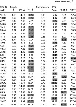Shown are rmsds between reference graphs from solved structures and our sampled graphs by MC/SA—initial, lowest score (P2, restricted moves) and lowest cluster representative (P3, random moves) after MC/SA—along with correlation coefficients between rmsd and score (r). Compared with predictions by MC-Sym (2), FARNA (3), and NAST (1), best rmsds for our P2 are shown in bold, and our P3 in gray highlight. See SI Appendix, Table S2 for other assessment protocols (N/A, program fails).

Results

We assess candidate graphs before and after MC/SA for our 30 test RNAs in Table 1 and SI Appendix, Table S2 and Fig. S6. After MC/SA, we compare results to 3D graphs of solved RNAs by three procedures (P1–P3). P1 directly compares the lowest-graph rmsd among the final pool of accepted graphs to the reference graph translated from the solved structure. P2 compares our lowest-scored graph among accepted graphs to the reference graph. For random moves, conformational space is more globally sampled compared with restricted moves, and additional clustering is required to select a representative graph from among five clusters (P3) (Fig. 3). We choose five clusters because this yields silhouette coefficients (24) greater than 0.4 for all 30 RNAs, indicating satisfactory clustering (SI Appendix, Table S3). These procedures uncover interesting relationships between rmsd/score landscape and the nature of the RNA (self-folding, protein-binding, etc.). Because prior work (23) and our statistical analyses here show that graph rmsds are positively correlated to all-atom rmsds, our assessment of candidate topologies based on graph rmsd is fair.

Fig. 3.

Predicted graphs before and after MC/SA based on random pivot moves—best graph with lowest rmsd from reference graph (P1), lowest-scored graph (P2), and lowest cluster representative (P3) of landscapes with respect to lowest-scored graph for (A) 1MJI (34 nt, 5S rRNA), (B) 2PXB (49 nt, signal recognition particle), (C) 1LNG (97 nt, signal recognition particle), and (D) 1GID (158 nt, group I intron P4–P6). Gray highlights indicate lower rmsds than all-atom predictions. Landscapes with respect to lowest-scored graphs and native structure are also shown. See SI Appendix, Fig. S9 for graph results for all 30 test RNAs.

Graphs Before MC/SA Sampling.

Following graph scaling by size measures and junction predictions by RNAJAG (23), our graphs present reasonable starting candidate topologies for MC/SA. Table 1 shows that initial graph rmsds range from 2.42 [Protein Data Bank (PDB) ID code 2IPY] to 46.11 Å (PDB ID code 1GID).

Though internal loop geometries are further optimized by MC sampling, edge lengths and imperfect junction predictions are not changed further. Edge lengths are mostly well-estimated except for RNAs bound to proteins or other ligands. For example, the estimated edge length for the internal loop of the box C/D RNA–protein complex (1RLG) is short (19.9 Å vs. 24.8 Å).

For RNAs with junctions (12 of 30 test RNAs), junction families and coaxial stacking are generally predicted well by RNAJAG (23) based on a collective training set of 244 junctions. RNAJAG was developed by a 10-fold cross-validation that excluded each junction in turn when predicting its topology. That protocol yielded good accuracy: prediction accuracy for coaxial stacking was 95%/92% in three-way/four-way junctions and, for family type, 94%/87% in three-way/four-way junctions (23). However, for the unique junction topology 1LNG not represented by other junctions in the training set, family A and coaxial stacking in H1H2 were predicted instead of correct family C and coaxial stacking in H1H3 (23), as also predicted here using the collective training set. (If this incorrect junction would have been used here, there would be 23.77 Å rmsd before MC/SA compared with 6.20 Å in Table 1 and 17.12 Å after MC/SA compared with 14.56 Å in Table 1.) Note that even when a correct junction topology is predicted, geometric differences can result with respect to helix orientations. Overall, size measures and junction predictions provide good starting points for MC/SA, which tends to improve the internal loop geometries and overall 3D topologies.

Graphs After MC/SA Sampling with Knowledge of Reference Graphs.

For our 30 test RNAs, we run 10⁴ steps of MC for both restricted pivot moves (which converge to one region of conformational space) and random pivot moves (which explore multiple regions of space and thus requires clustering analysis; SI Appendix, Figs. S7 and S8). The total acceptance ratio is 40–60% for the former and 30–50% for the latter.

For rmsds relative to reference graphs (P1 in SI Appendix, Table S2), lowest values range from 1.37 Å (1I6U) to 14.56 Å (1GID) using restricted moves (<6 Å for 25 of 30 RNAs) and 1.30 Å (2PXB) to 12.57 Å (2LKR) using random moves (<6 Å for 26 of 30 RNAs). Thus, graph sampling using knowledge-based statistical potentials can approach reasonably the topology of native-like RNAs. Fig. 3 and SI Appendix, Fig. S9 present corresponding landscapes—score vs. rmsd from experimental structure graph and score vs. rmsd from lowest-scored graph. These landscapes indicate downhill shapes when the experimental structure is known for most RNAs except protein-bound RNAs and RNAs with inaccurate junction predictions. When lowest-scored graph is used as reference instead, all landscapes are downhill in shape by design.

Assessment of MC/SA Results Without Knowledge of Reference Graphs.

In a true prediction, the reference graph is not known, and lowest scores can be used instead. Our analysis shows that whereas low-scored clusters correlate to low rmsds, individual scores do not always correspond to lowest rmsds (Table 1). Thus, we consider both lowest-scored graphs (P2) and lowest-scored graph representatives among five clusters (P3, for random moves) as references for the rmsds given in Table 1 and SI Appendix, Table S2.

For P2, graph rmsds range from 2.38 Å (2IPY) to 30.89 Å (2LKR) for restricted moves (P2 in Table 1) and 2.29 Å (2IPY) to 28.63 Å (1GID) for random moves (P2 in SI Appendix, Table S2). Although these graph rmsds are higher than lowest rmsds compared with solved RNAs (P1 in SI Appendix, Table S2), lowest scores provide reasonable predictions of RNA 3D topologies.

Fig. 3 and SI Appendix, Fig. S9 show clustered landscapes with respect to graph rmsds from lowest-scored graphs based on random moves. Representative graphs from five clusters sorted by score from low to high offer candidate 3D topologies in the absence of solutions (SI Appendix, Table S4). For example, for L1 protein–mRNA binding RNA (1ZHO), the lowest-scored graph has 7.46 Å but the representative graph of cluster 3 has 3.99 Å. For most cases, representative graphs with lower scores have low rmsds from the reference graph (SI Appendix, Table S4). Representative graphs from cluster 1 have rmsds ranging from 2.52 Å (1I6U) to 28.24 Å (1GID) (P3 in Table 1), similar to lowest-scored graphs (P2).

To understand these clustering results, we investigate in Fig. 4 and Table 1 landscapes with respect to graph rmsd from native structures and the correlation coefficient, r, between score and graph rmsd from native structures (r ranges from −1 to 1). A positive coefficient indicates high accuracy; a coefficient near zero indicates no correlation between graph rmsd and score; and a negative coefficient indicates a less-accurate prediction than random selection. For 25 of 30 cases, we have positive correlations between graph rmsd and score (Table 1), with 16 having r > 0.5 and classic downhill landscapes. For example, the iron-responsive element (2IPY) has r = 0.96 (Fig. 4A). For protein-binding RNAs or inaccurate junction topology cases, the correlation is neutral (i.e., ) or negative. In these cases, corresponding landscapes are downhill in part or flat. For example, mRNA–L1 ribosomal RNA complex (1ZHO) and the thiamine pyrophosphate riboswitch with three-way junction (3D2G) have values of 0.2 and −0.42, respectively (Fig. 4 B and C).

Fig. 4.

Clustered energy landscape and correlation between score and graph rmsd from native structure for three cases. (A) Typical positive correlation (2IPY, r = 0.96, also for 1OOA, 2IPY, 1MJI, 1I6U, 1F1T, 1S03, 1XJR, 2PXB, 2OIU, 1MZP, 2HGH, 1DK1, 1D4R, 1KXK, 1P5O, and 1MFQ). (B) Neutral correlation (1ZHO, r = 0.20, also for 1RLG, 2OZB, 2HW8, 1ZHO, 1U63, 1SJ4, 2LKR, and 1GID). (C) Negative correlation (3D2G, r = –0.42, also for 1MMS, 3D2G, 2HOJ, 2GDI, and 2GIS). Red horizontal lines mark scores of the native structure. (Lower) Representative graphs (red) from clusters with native-like scores are superimposed upon solved structures (gray).

Comparison with Other Tools.

Programs MC-Sym (2), FARNA (3), and NAST (1) produce all-atom models from 2D structures based on fragment libraries (MC-Sym and FARNA) or one-bead models (NAST). Though these tools predict small structures (<40 nt) reasonably, errors increase as RNA lengths increase (6). Here, we translate predicted all-atom models from these programs to 3D graphs and compute graph rmsds between these graphs and our predictions in Table 1 and SI Appendix, Table S2. We had already showed that graph rmsds are comparable to all-atom rmsds in junctions (23) (see also below).

For lowest rmsd graphs (P1), our candidates have the lowest graph rmsds for 27 of 30 RNAs for both MC/SA protocols. For the three RNAs (2IPY, 1S03, and 2GIS), the difference in graph rmsd between our approach and the other tools is less than 0.7 Å. For lowest-scored graphs (P2), our approach outperforms other programs for 16 and 14 of 30 RNAs, for restricted and random moves, respectively; our lowest cluster representatives (P3) based on random moves similarly yield 16 of 30 RNAs with lowest rmsd among all predictions; MC-Sym, FARNA, and NAST have best results for seven, five, and two structures, respectively (Table 1). Thus, our P2 based on restricted moves and P3 (with random moves) emerge as best approaches when the solution is not known.

How valid is our assessment of candidate graphs with respect to predicted graphs (translated from solved structures) rather than predicted atomic models vs. solved atomic models? To supplement our discussion of this point in ref. 23, we analyze correlations between graph and all-atom rmsds using results from three all-atom modeling tools for 30 RNAs in SI Appendix, Fig. S10: graph and atomic rmsds are positively correlated; the slope from the linear regression of graph rmsd with respect to all-atom models is 0.89. For example, the graph and all-atom rmsds of 1MFQ are very similar: 35.94 Å and 35.28 Å for MC-Sym; 21.30 Å and 16.48 Å for FARNA; and 29.64 Å and 27.76 Å for NAST. However, graph rmsds are smaller than all-atom rmsds (intercept value of the linear regression of graph rmsd with respect to all-atom rmsd is −3.10), because vertices rather than atoms are compared, and terminal regions that exhibit variations are not compared. Thus, overall similarity between structures can be captured by graph rmsds.

Discussion

We have presented a hierarchical computational approach for one aspect of the challenging task of RNA structure prediction by predicting global helical arrangements in RNA using graph sampling. First, we define RNA 3D graphs by representing helix ends and unpaired regions as vertices and connecting them by edges, thereby capturing both 2D topologies and 3D geometries. Second, we develop knowledge-based potentials to connect 2D topologies to their 3D geometries. Third, we set up initial planar graphs embedded in 3D from a given 2D structure based on junction prediction and edge length estimation using RNAJAG (23). Fourth, we sample graph conformations in 3D space by MC/SA based on restricted or random pivot moves, score them by our statistical potentials, and predict global helical arrangements using clustering analysis. The final predictions consist of graphs or graph cluster representatives, which we compare with graphs of the solved structure (P1) or to our lowest-scored graphs (P2 and P3).

RNA 3D graphs allow us to quantify 3D global geometrical features such as size and helical angles. The distributions of 3D geometrical parameters correlate to 2D structures, which provide a reasonable scoring system for predicting preferences of helical arrangements. Our sampling based on geometric statistical potentials produces graphs whose 3D shapes resemble native structures, and the lowest-scored graphs are also reasonably selected without knowledge of reference graphs. In most cases, the relationship between scores and graph rmsd from native structures is positive, so the lowest-scored cluster representative predicts 3D topologies close to the native structures (Table 1). Several structures including protein-binding RNAs (e.g., 1RLG, 1MJI, and 1ZHO) are better predicted by other representative graphs in higher-scored clusters; in these cases, our scores and graph rmsds from native structures have neutral or negative correlations. In general, rmsd values are larger for RNAs than proteins because RNAs occupy more volume per unit mass compared with proteins, and thus small perturbations in RNA can induce large rmsds.

Our approach exploits coarse-grained graph motifs to reduce the conformational space significantly to facilitate a systematic search in global topology space. Our MC/SA sampling protocols sample RNA-like graphs efficiently: compared with other all-atom prediction tools, our lowest-rmsd graphs have best graph rmsds for 27 of 30 test RNAs. Without knowledge of reference graphs, our lowest-scored graphs or lowest-cluster representatives yield best rmsds for more than half (∼16) of the RNAs (compared with seven or less for other prediction tools). Because graph rmsds are positively correlated to all-atom rmsds (SI Appendix, Fig. S10), a comparison between graphs rather than atomic models is reasonable to assess the accuracy of prediction (23).

Though 3D tree graphs cannot handle pseudoknots, we can approximate global interactions due to pseudoknots by closer distances between the two interconnected strands. The distance between two loops when they form a pseudoknot is small, as shown in reference graphs and lowest-rmsd graphs of rRNA fragment (1MZP) and hepatitis delta virus ribozyme (1SJ4) in SI Appendix, Fig. S9. The loop–loop, loop–helix, helix–helix distances can further suggest other long-range interactions (e.g., kissing loops, loop–receptor, A-minor).

Of course, atomic models rather than 3D graphs are ultimately desired. Our hierarchical method based on graph partitioning shows that this translation into atomic models is feasible (23). Our build-up approach based on 3D-RAG, an extension of the RAG database containing solved 3D coordinates, essentially combines 3D fragments of subgraphs associated with 3D coordinates based on a search for graph isomorphisms. We select a graph partitioning based on lowest rmsds with corresponding 3D coordinates of the subgraph, add or substitute bases to match the target subsequences, and merge the substructures to form a final all-atom candidate for the entire target graph (Fig. 1D). This model can be further relaxed by energy minimization or dynamics simulations.

Our restricted-move protocol P2 and clustering approach P3 using lowest scores among five clusters work well (Table 1, Figs. 3 and 4, and SI Appendix, Fig. S9). For protein-free RNAs, correlations between graph rmsds and scores are positive. However, improvements can be envisioned to account for nondownhill landscapes in the case of protein-binding and junction structures. Namely, the scoring function values for size, bending, and torsion angles could be different from protein-free cases. In addition, our prediction of RNA junctions could be extended from the current three discrete models: parallel , perpendicular , and diagonal helical arrangements because helical orientations are continuous rather than discrete.

Our hierarchical graph-sampling approach already serves well as a first-order approximation for large RNAs. To better predict large and complex RNAs, ongoing work includes determination of higher-order junction topologies, exhaustive rather than stochastic sampling of 3D graph space, and improvement of scoring functions based on geometrical parameters containing long-range interactions as well as separation of self-folding RNA parameters from those for protein- or substrate-binding RNAs. Combined with other improvements such as more accurate 2D folding algorithms, our hierarchical graph-sampling approach could address 3D topology predictions for large RNAs.

Materials and Methods

Full details can be found in SI Appendix.

Junction Prediction.

We determine the coordinates of junction vertices (one for the junction loop center and 2n for n-way helices) using the RNAJAG program (23). RNAJAG predicts three- and four-way junction topologies as a function of sequence and length using a random forest data-mining approach with a 10-fold cross-validation procedure trained by known junctions. Here we use a collective training set including all 244 known junctions to develop a uniform junction prediction protocol applicable to all RNAs. The three-way junctions are classified into three families by helical configurations: A (perpendicular), B (diagonal), and C (parallel) (SI Appendix, Fig. S2) (25). The four-way junctions are classified into nine major families: H, cH, cL, cK, π, cW, ψ, cX, and X (26). See SI Appendix, Fig. S2 for H (parallel), cH (crossed and parallel), π (diagonal), and cL (crossed and perpendicular) families. Once the junction topologies are determined, RNAJAG sets up the coordinates of junction vertices for initial planar tree graphs by the size measures.

MC/SA Sampling of 3D Graphs.

We use hierarchical sampling approaches using our knowledge-based statistical potentials built from bending and torsion angles of internal loops and radii of gyration based on RNA 3D graphs. See SI Appendix for a detailed description of RNA 3D graphs and statistical potentials. The MC/SA consists of three steps: (i) set-up of initial tree graphs given a 2D structure using size measures and junction prediction; (ii) MC/SA sampling of RNA 3D graphs with two types of move protocols (restricted pivot moves reciprocally decreasing angle ranges from 360° to 10° along MC steps and random pivot moves) guided by the potential scores: if the score for a new conformation is lower than that of the old conformation, the new conformation is accepted. If the new score is higher, the simulated annealing sampling proceeds: the move for each step j is accepted with probability , where E_j is the score difference from new to old conformations and the decreasing system temperature T_j = c/log₂(1 + j/s) where s is the total MC step, and c = 1/4log₂(10) (for restricted moves) or c = 1/log₂(10) (for random moves); (iii) assessment of resulting sampled graphs by three procedures: lowest rmsd from known structures (P1), lowest-scored graph (P2), and lowest-scored cluster representative for five clusters (P3).

References

- 1.Jonikas MA, et al. Coarse-grained modeling of large RNA molecules with knowledge-based potentials and structural filters. RNA. 2009;15(2):189–199. doi: 10.1261/rna.1270809. [DOI] [PMC free article] [PubMed] [Google Scholar]
- 2.Parisien M, Major F. The MC-Fold and MC-Sym pipeline infers RNA structure from sequence data. Nature. 2008;452(7183):51–55. doi: 10.1038/nature06684. [DOI] [PubMed] [Google Scholar]
- 3.Das R, Baker D. Automated de novo prediction of native-like RNA tertiary structures. Proc Natl Acad Sci USA. 2007;104(37):14664–14669. doi: 10.1073/pnas.0703836104. [DOI] [PMC free article] [PubMed] [Google Scholar]
- 4.Sharma S, Ding F, Dokholyan NV. iFoldRNA: Three-dimensional RNA structure prediction and folding. Bioinformatics. 2008;24(17):1951–1952. doi: 10.1093/bioinformatics/btn328. [DOI] [PMC free article] [PubMed] [Google Scholar]
- 5.Sim AY, Levitt M, Minary P. Modeling and design by hierarchical natural moves. Proc Natl Acad Sci USA. 2012;109(8):2890–2895. doi: 10.1073/pnas.1119918109. [DOI] [PMC free article] [PubMed] [Google Scholar]
- 6.Laing C, Schlick T. Computational approaches to 3D modeling of RNA. J Phys Condens Matter. 2010;22(28):283101–283118. doi: 10.1088/0953-8984/22/28/283101. [DOI] [PMC free article] [PubMed] [Google Scholar]
- 7.Bailor MH, Mustoe AM, Brooks CL, 3rd, Al-Hashimi HM. 3D maps of RNA interhelical junctions. Nat Protoc. 2011;6(10):1536–1545. doi: 10.1038/nprot.2011.385. [DOI] [PMC free article] [PubMed] [Google Scholar]
- 8.Tang RS, Draper DE. Bulge loops used to measure the helical twist of RNA in solution. Biochemistry. 1990;29(22):5232–5237. doi: 10.1021/bi00474a003. [DOI] [PubMed] [Google Scholar]
- 9.Friederich MW, Gast FU, Vacano E, Hagerman PJ. Determination of the angle between the anticodon and aminoacyl acceptor stems of yeast phenylalanyl tRNA in solution. Proc Natl Acad Sci USA. 1995;92(11):4803–4807. doi: 10.1073/pnas.92.11.4803. [DOI] [PMC free article] [PubMed] [Google Scholar]
- 10.Zheng G, Lu XJ, Olson WK. Web 3DNA—a web server for the analysis, reconstruction, and visualization of three-dimensional nucleic-acid structures. Nucleic Acids Res. 2009;37(Suppl 2):W240–W246. doi: 10.1093/nar/gkp358. [DOI] [PMC free article] [PubMed] [Google Scholar]
- 11.Humphris-Narayanan E, Pyle AM. Discrete RNA libraries from pseudo-torsional space. J Mol Biol. 2012;421(1):6–26. doi: 10.1016/j.jmb.2012.03.002. [DOI] [PMC free article] [PubMed] [Google Scholar]
- 12.Sim AY, Levitt M. Clustering to identify RNA conformations constrained by secondary structure. Proc Natl Acad Sci USA. 2011;108(9):3590–3595. doi: 10.1073/pnas.1018653108. [DOI] [PMC free article] [PubMed] [Google Scholar]
- 13.Waterman MS. Secondary structure of single-stranded nucleic acids. Adv Math Suppl Studies. 1978;1:167–212. [Google Scholar]
- 14.Le SY, Nussinov R, Maizel JV. Tree graphs of RNA secondary structures and their comparisons. Comput Biomed Res. 1989;22(5):461–473. doi: 10.1016/0010-4809(89)90039-6. [DOI] [PubMed] [Google Scholar]
- 15.Shapiro BA, Zhang KZ. Comparing multiple RNA secondary structures using tree comparisons. Comput Appl Biosci. 1990;6(4):309–318. doi: 10.1093/bioinformatics/6.4.309. [DOI] [PubMed] [Google Scholar]
- 16.Kim N, Fuhr KN, Schlick T. Graph applications to RNA structure and function. In: Russell R, editor. Biophysics of RNA Folding. New York: Springer; 2012. [Google Scholar]
- 17.Kim N, Petingi L, Schlick T. Network theory tools for RNA modeling. WSEAS Trans Math. 2013;12(9):941–955. [PMC free article] [PubMed] [Google Scholar]
- 18.Izzo JA, Kim N, Elmetwaly S, Schlick T. RAG: An update to the RNA-As-Graphs resource. BMC Bioinformatics. 2011;12:219. doi: 10.1186/1471-2105-12-219. [DOI] [PMC free article] [PubMed] [Google Scholar]
- 19.Koessler DR, Knisley DJ, Knisley J, Haynes T. A predictive model for secondary RNA structure using graph theory and a neural network. BMC Bioinformatics. 2010;11(Suppl 6):S21. doi: 10.1186/1471-2105-11-S6-S21. [DOI] [PMC free article] [PubMed] [Google Scholar]
- 20.Kim N, Izzo JA, Elmetwaly S, Gan HH, Schlick T. Computational generation and screening of RNA motifs in large nucleotide sequence pools. Nucleic Acids Res. 2010;38(13):e139. doi: 10.1093/nar/gkq282. [DOI] [PMC free article] [PubMed] [Google Scholar]
- 21.Gopal A, Zhou ZH, Knobler CM, Gelbart WM. Visualizing large RNA molecules in solution. RNA. 2012;18(2):284–299. doi: 10.1261/rna.027557.111. [DOI] [PMC free article] [PubMed] [Google Scholar]
- 22.Quarta G, Kim N, Izzo JA, Schlick T. Analysis of riboswitch structure and function by an energy landscape framework. J Mol Biol. 2009;393(4):993–1003. doi: 10.1016/j.jmb.2009.08.062. [DOI] [PMC free article] [PubMed] [Google Scholar]
- 23.Laing C, et al. Predicting helical topologies in RNA junctions as tree graphs. PLoS ONE. 2013;8(8):e71947. doi: 10.1371/journal.pone.0071947. [DOI] [PMC free article] [PubMed] [Google Scholar]
- 24.Kaufman L, Rousseeuw PJ. Finding Groups in Data: An Introduction to Cluster Analysis. New York: Wiley; 1990. [Google Scholar]
- 25.Lescoute A, Westhof E. Topology of three-way junctions in folded RNAs. RNA. 2006;12(1):83–93. doi: 10.1261/rna.2208106. [DOI] [PMC free article] [PubMed] [Google Scholar]
- 26.Laing C, Schlick T. Analysis of four-way junctions in RNA structures. J Mol Biol. 2009;390(3):547–559. doi: 10.1016/j.jmb.2009.04.084. [DOI] [PMC free article] [PubMed] [Google Scholar]
- 27.Schlick T. A modular strategy for generating starting conformations and data-structures of polynucleotide helices for potential-energy calculations. J Comput Chem. 1988;9(8):861–889. [Google Scholar]
Associated Data
This section collects any data citations, data availability statements, or supplementary materials included in this article.