Scaling of Perceptual Errors Can Predict the Shape of Neural Tuning Curves

Abstract

Weber’s law, first characterized in the 19th century, states that errors estimating the magnitude of perceptual stimuli scale linearly with stimulus intensity. This linear relationship is found in most sensory modalities, generalizes to temporal interval estimation, and even applies to some abstract variables. Despite its generality and long experimental history, the neural basis of Weber’s law remains unknown. This work presents a simple theory explaining the conditions under which Weber’s law can result from neural variability and predicts that the tuning curves of neural populations which adhere to Weber’s law will have a log-power form with parameters that depend on spike-count statistics. The prevalence of Weber’s law suggests that it might be optimal in some sense. We examine this possibility, using variational calculus, and show that Weber’s law is optimal only when observed real-world variables exhibit power-law statistics with a specific exponent. Our theory explains how physiology gives rise to the behaviorally characterized Weber’s law and may represent a general governing principle relating perception to neural activity.

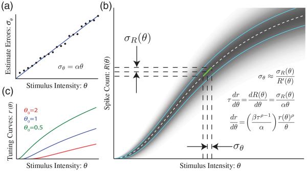
Relating behavior and perception to underlying neuronal processes is a major goal of systems neuroscience [1]. The ability to estimate the magnitudes of external stimuli (the intensity of a light, for example) is a fundamental component of perception and inherently prone to error. Interestingly, for many variables, magnitude estimate errors scale linearly with stimulus magnitude [Fig. 1(a)]. This relationship, called Weber’s law [2], has proven robust and ubiquitous across sensory modalities, holds in the temporal domain (where it is called scalar timing [3,4]), and even applies to abstract quantities associated with decision making [5] and numerosity [6]. Despite the long history of this observation, its prevalence, and its perceived importance, the physiological basis of Weber’s law is unknown.

FIG. 1.

Weber’s law and neuronal statistics. (a) Weber’s law [Eq. (2)] states that stimulus intensity estimate errors (σ_θ, solid line indicating the fit of the schematic data points) increase linearly with physical stimulus intensity (described by the parameter θ) with a slope defined as the Weber fraction α. (b) A linear approximation [green line, Eq. (2)] relates the standard deviation of the spike-count distribution to the standard deviation of the error in estimating the magnitude variable θ. (c) Example tuning curves with Poisson spike statistics for different values of the integration constant θ₀. Solutions that decrease with θ can also be obtained; see Supplemental Fig. S1 [15].

Various attempts have been made to formulate theoretical frameworks that can explain Weber’s law. For example, soon after Weber’s law was observed experimentally [2], Fechner postulated the existence of a hypothetical “subjective sense of intensity” that varies logarithmically with the physical intensity of a stimulus [7]. In this work, rather than searching for a hypothetical variable, we address the issue by asking what properties realistic physiological variables (i.e., neuronal spike trains) must have to account for the experimental data.

Our analysis starts with the assumption that an external sensory stimulus θ is represented in the nervous system by a stochastic spiking neural process with firing rate r(θ) that varies monotonically with the magnitude of θ [Fig. 1(b)]. We further assume that a windowed spike count of this process R is used by the brain on a trial-by-trial basis to make a magnitude estimate θ_est. Estimate errors, in this formulation, result from stochastic fluctuations of R. The phrase “neural process” is used as a generic term that could describe anything ranging from a single neuron to a large ensemble of neurons (although there is good reason to assume it refers to a neural population; see the discussion below).

The magnitude of errors estimating parameter θ from the spike count can be linearly approximated [Fig. 1(b)] as

$${\sigma }_{\theta }\left(\theta \right)\approx \frac{{\sigma }_R\left(\theta \right)}{\mid R^{\prime }\left(\theta \right)\mid }=\frac{{\sigma }_R\left(\theta \right)}{\mid \tau r^{\prime }\left(\theta \right)\mid },$$ (1)

where σ_θ is the standard deviation of stimulus estimates, σ_R(θ) is the standard deviation of the spike count at parameter θ, R′(θ) is the derivative of the spike-count curve with respect to parameter θ, and τ is the estimate window width (i.e., the per-trial duration around an external stimulus event over which spike counts are accumulated). According to Weber’s law, errors estimating θ scale linearly with θ. Using standard deviation as the error measure, this is written as

$${\sigma }_{\theta }\left(\theta \right)=\alpha \theta ,$$ (2)

where α is called the Weber fraction (which is determined experimentally by measuring behavioral performance).

We can now relate errors within the physiologic process assumed to underlie perception with experimentally measured perceptual performance by combining Eqs. (1) and (2):

$$\tau \frac{dr}{d\theta }=\frac{dR\left(\theta \right)}{d\theta }=\pm \frac{{\sigma }_R\left(\theta \right)}{\alpha \theta },$$ (3)

where the plus sign is valid when the slope of r(θ) is positive and the minus sign is valid when it is negative.

Spike-count variability can be described using a power-law model [8,9] with the form

$${\sigma }_R\left(\theta \right)=\beta {\left(\tau r\left(\theta \right)\right)}^{\rho }.$$ (4)

Substituting Eq. (4) into (3) results in

$$\frac{dr\left(\theta \right)}{d\theta }=\pm \left(\frac{\beta {\tau }^{\rho -1}}{\alpha }\right)\frac{r{\left(\theta \right)}^{\rho }}{\theta }.$$ (5)

The solution of Eq. (5) has a log-power form

$$r\left(\theta \right)=K{[\pm \text{ln}(\theta ∕{\theta }_0)]}^n,$$ (6)

where $K=\frac{1}{\tau }{[\beta (1-\rho )∕\alpha ]}^n$ and $n=\frac{1}{1-\rho }$. This relationship holds whether r rises (θ ≥ θ₀, + case) or falls (θ < θ₀, − case) monotonically. The parameter θ₀, an integration constant, actually determines the detection threshold. The solution to Eq. (5) defines the shape of neural tuning curves (e.g., input-output relationships) that will, under the minimal assumptions and approximations outlined above, result in a linear increase in perceptual errors with stimulus magnitude. Another way of looking at this is that the form of this equation restricts the class of tuning curves for neural processes that display Weber’s law to the log-power form of Eq. (6). Note that all the parameters are determined either by the spike statistics (i.e., the physiology) or the behavioral performance (i.e., the Weber fraction α).

The general log-power form takes on a specific shape, depending primarily on the form of the spike-count statistics. In the constant noise case (ρ = 0), this equation reduces to Fechner’s law [7]. Hence, Fechner’s law can be seen as making an implicit constant noise assumption. In the special and unrealistic case where ρ = 1, a power-law solution is obtained [10].

Experimentally, a nearly linear relationship between mean spike count and variance is commonly observed [8,9,11]. In this nearly Poisson case (ρ = 1/2), one obtains a log-power law with an exponent of n = 2. Examples of tuning curves for the Poisson statistics are shown in Fig. 1(c) for the monotonically increasing case.

Given a tuning curve [r(θ)] and spike probability distribution (P_s), one can calculate the exact standard deviation of the estimate errors as a function of the estimated variable’s magnitude. To test the validity of our linear approximation, we derived the mean and the standard deviation of the noisy estimates, assuming Poisson spike statistics with appropriate log-power tuning curves. The mean number of spike for a time interval τ is τr(θ), and the probability of having k spikes in a single trial is P_s[k|τ * r(θ)]. Given that there are k_i spikes in trial i, the inverse of the tuning curve can be used to estimate θ_est(i) = r⁻¹(k_i/τ). The mean estimated parameter θ_est is therefore

$$\langle {\theta }_{\text{est}}\rangle =\sum _k{P}_s[k\mid \tau r\left(\theta \right)]r^{-1}(k∕\tau )$$ (7)

and the variance of the estimate is

$${\sigma }_{\theta }^2=\sum _k{P}_s[k\mid \tau r\left(\theta \right)]{[r^{-1}(k∕\tau )-\langle {\theta }_{\text{est}}\rangle ]}^2.$$ (8)

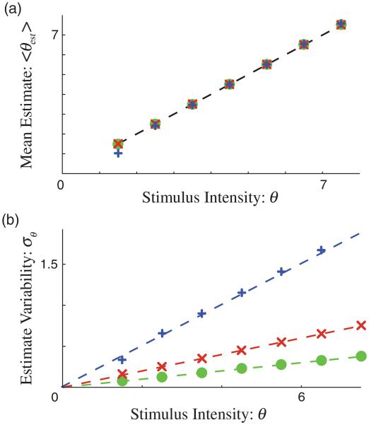
If the spike statistics are well approximated by a Poisson process (ρ = 1/2, β = 1), then P_s is the Poisson distribution. These calculations show that log-power tuning curves produce excellent approximations to both the mean [Fig. 2(a)] and the linear scaling of the standard deviation [Fig. 2(b)]. The linear approximation provides a nearly perfect agreement with the exact solution for low α values. A small discrepancy exists for larger values of α, which are less realistic and correspond to higher noise levels, but only for values of θ near the lowest limit. Similar calculations can also be carried out for non-Poisson distributions by changing the functional form of P_s.

FIG. 2.

Weber’s law with Poisson statistics. (a) The mean stimulus estimation as a function of the true target parameter. For small α values [α = 0:05 (green circles), 0.1 (red crosses), 0.25 (blue + symbols)], the estimate is nearly perfect. (b) The standard deviation of the parameter estimate scales linearly with the mean as a function of α (shown for a monotonically rising r function with θ₀ = 1, τ = 0.5, β = 1, and ρ = 0.5).

It is difficult to make explicit sensory magnitude estimates. For this reason, psychophysical experiments typically employ the “just noticeable difference” (JND) methodology to measure perception. In this paradigm, subjects are asked to judge the intensity of test stimuli (θ_t) relative to a reference stimulus (θ_r). Test stimuli are selected in a range around a fixed reference stimulus and varied to find the values at which the subject perceives that the test stimulus is larger than the reference in 75% (θ₁) and 25% (θ₂) of the trials. The JND metric is defined as (θ₁ − θ₂)/2 [7,12].

This definition of JND can be used to compute an equivalent metric for our model. To do so, we use the tuning curve r and the probability distribution function P_s to generate spike counts n_r and n_t for reference and test stimuli, respectively. Assuming, for simplicity, a deterministic n_r = τr(θ_r), the probability that the a test stimulus will elicit more spikes than the reference stimulus is

$$P_g({\theta }_r\mid n_r)=\sum _{n>n_r}{P}_s(n\mid \tau r\left({\theta }_t\right)).$$ (9)

As described above, θ₁ is the value of θ_t at which n_t > n_r 75% of the time. Formally,

$${\theta }_1\left(n_r\right)={\text{arg}}_{{\theta }_t}\{P_g({\theta }_t\mid n_r)=0.75\}$$ (10)

and similarly

$${\theta }_2\left(n_r\right)={\text{arg}}_{{\theta }_t}\{P_g({\theta }_t\mid n_r)=0.25\}.$$ (11)

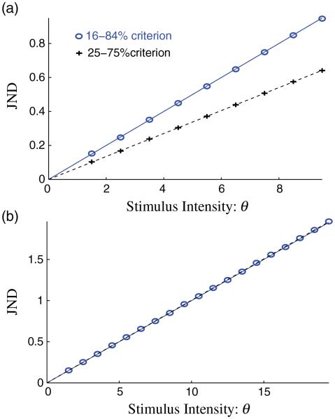
Using these definitions, we find that the JND scales linearly with the magnitude of θ but with a slope different than the slope of the standard deviation [Fig. 3(a), + symbols]. The reason for the discrepancy is that, while the JND spans 50% of the probability distribution (from 25% to 75%), the standard deviation of a Gaussian distribution spans 68% of the distribution (from 16% to 84%). If we change the criteria in the equations above to match this observation, we obtain results that match predictions of the linear theory almost exactly [Fig. 3(a), ∘ symbols]. This striking agreement occurs because the number of spikes generated by the Poisson process in this example is well approximated by a Gaussian. Higher α values will produce lower spike rates and a commensurately larger discrepancy between the standard deviation and the JND slopes.

FIG. 3.

Linear scaling of the JND. (a) The JND, assuming a fixed number of spikes in the reference stimulus. When the JND is calculated in the range from 25% to 75% (+ symbols), it is still linear but with a smaller slope that the standard deviation. When the range is corrected to 16% to 84% (∘ symbols), a slope identical to the standard deviation of the error is found. (b) When fluctuations in the number of reference spikes are taken into account, we find that the theory produces an identical slope to that found for the linear theory and the mean reference spike number. (Here, we used the 16%–84% interval.) The results shown are with α = 0.1.

To better replicate the experimental procedure, we can calculate the JND using a value of n_r stochastically drawn from the same distribution that generates n_t. In this case, θ₁(n_r) and θ₂(n_r) are replaced by ${\stackrel{‒}{\theta }}_1={\sum }_{n_r}{P}_s\left(n_r\right){\theta }_1\left(n_r\right)$ and ${\stackrel{‒}{\theta }}_2={\sum }_{n_r}{P}_s\left(n_r\right){\theta }_2\left(n_r\right)$. Figure 3(b) shows the results produced with these definitions using the the 16%–84% interval. Surprisingly, these results are identical to those obtained when we assumed a deterministic number of reference spikes. This agreement occurs because θ₁ and θ₂ depend nearly linearly on the fluctuations in the number of reference spikes; arising from a symmetric distribution, fluctuations in one direction are balanced by fluctuations in the other direction. These results indicate that log-power tuning curves produce linear scaling of the error measure as postulated by Weber’s law for various error estimation methods, including those used experimentally.

It is sometimes found that scaling is not perfectly linear [13,14] but can be described with a power-law form

$${\sigma }_{\theta }\left(\theta \right)=\alpha {\theta }^{1-\varphi },$$ (12)

where ϕ is a correction term to the perfect linear scaling of Weber’s law. This results in a differential equation of the form

$$\frac{dr\left(\theta \right)}{d\theta }=\pm \left(\frac{\beta {\tau }^{\rho -1}}{\alpha }\right)\frac{r{\left(\theta \right)}^{\rho }}{{\theta }^{1-\varphi }}.$$ (13)

This ordinary differential equation has a power-law solution of the form

$$r\left(\theta \right)=K_1{\left(\frac{{\theta }^{\varphi }}{\varphi }-\frac{{\theta }_0^{\varphi }}{\varphi }\right)}^n,$$ (14)

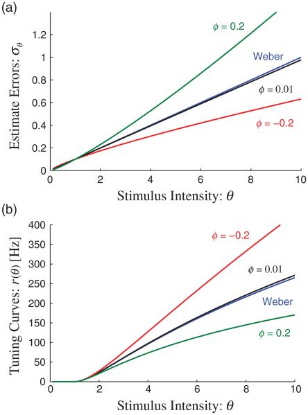
where K₁ = [±β(1 − ρ)/α]ⁿ/τ and θ₀ is as above both the integration constant and the detection threshold. As in the log-power case, there are two valid solutions: a monotonically increasing solution above θ₀ and a monotonically decreasing solution below θ₀. In the limit ϕ → 0, Eq. (14) converges to Eq. (6). The solutions nearly overlap when ϕ is small but diverge as ϕ increases to higher values [Fig. 4(b)]. Note that a power-law solution has been suggested as a good description of a subjective sense of intensity [10]. This result demonstrates how our approach can be used to analytically obtain tuning curves for error scaling that is not perfectly linear; in fact, the linear case could be considered a special case of the more general solution. Similar procedures can be used for any functional form of error scaling or a spike-count variability model; although there is no guarantee of an analytical solution, numerical methods can always be used.

FIG. 4.

Nonlinear scaling of errors. (a) In some cases, errors do not scale linearly with the magnitude. Examples are shown for various values of the nonlinearity characterization parameter ϕ. (b) Different values of ϕ result in different tuning curve shapes.

It is unlikely that any cognitive or perceptual brain functions result from neural representations based on the activity of single neurons; it is much more likely that such processes are implemented by neural populations organized into functional coding assemblies. Further, there is no reason to assume that all of the neurons within a coding population would or should have identical tuning curves. However, it is trivial to show that a diverse population of statistically independent neurons that are chosen such that the sum of their tuning curve closely approximates the log-power curve will also exhibit Weber’s law (see Supplemental Fig. S2 [15]).

While our theory does not require that the tuning curve of single neurons have a log-power form, recording from single neurons is much easier methodologically than recording simultaneously from neural ensembles and this is a good place to start looking for experimental correlates of our predictions. Ideally, we would like to fit recorded spike rates for neurons whose activity is tied to perceptual behavior for a stimulus that adheres to Weber’s law. Unfortunately, such a data set is hard to find in the literature. Published tuning curves as a function of stimulus contrast [8,16] can sometimes be well approximated by a log-power function with exponents close to those predicted above for realistic spike statistics (Supplemental Fig. S3 [15]). For other cells, the fits produce exponents that are inconsistent with observed spike statistics (Supplemental Fig. S3 [15]) or not well fit by log-power functions [17]. Contrast perception, however, is not a particularly good candidate to test our model, as it does not clearly display linear scaling.

As we have noted, Weber’s law is observed in many modalities and conditions. It is tempting to hypothesize that this universality reflects some sort of optimal strategy for minimizing average perceptual errors based on noisy spike-count statistics. For example, Weber’s law might be considered optimal if it minimizes the mean error of the estimated parameter. Mean error (E), defined simply as the weighted average of the standard deviation of the error at each value of θ, takes the mathematical form

$$E={\int }_{∊}^{\infty }{\sigma }_{\theta }\left(\theta \right)P\left(\theta \right)d\theta \approx {\int }_{∊}^{\infty }\left(\frac{R{\left(\theta \right)}^{\rho }}{\mid R^{\prime }\left(\theta \right)\mid }\right)P\left(\theta \right)d\theta ,$$ (15)

where P(θ) is the distribution of different expected magnitudes of the variable θ and ∊ is the minimal possible value of θ. The ≈ symbol is due to the linear error approximation described above.

We use variational calculus to find the function r(θ) which minimized the error while assuming a fixed distribution P(θ). The Euler-Lagrange equation [18] allows us to obtain the following differential equation for the functions r and P that minimize this error:

$$2\rho {\left(r^{\prime }\right)}^2-2r{r}^{″}+r{r}^{\prime }\frac{P^{\prime }}{P}=0,$$ (16)

where the prime symbols denote the derivative with respect to θ.

We can now use this equation to determine the form of P(θ) for which Weber’s law is optimal. We do this by plugging the functional form of the tuning curve r(θ) that yields linear scaling [Eq. (6)] directly into Eq. (16) to obtain

$$\left[\frac{2}{\theta }+\frac{P^{\prime }}{P}\right]r{r}^{\prime }=0,$$ (17)

which has the solution

$$P\left(\theta \right)=\frac{N}{{\theta }^2},$$ (18)

where N is the normalization constant, such that ${\int }_{∊}^{\infty }P\left(\theta \right)d\theta =1$. It is interesting to note that this function is independent of ρ. This result implies that Weber’s law is strictly optimal only if the statistics of the variable θ have a power-law form with an exponent of −2.

A similar procedure can be followed for other error functions. For example, if the relative error is chosen as the optimality criterion, then Weber’s law is optimal only when distribution has the form $P\left(\theta \right)\propto \frac{1}{\theta }$. While not all error functions will be minimized by a power-law distribution, for any reasonable error function definitions, optimality will depend on the statistics of the perceived world. Consequently, “optimal” tuning curves will also depend on the statistics of the world. For Weber’s law, which is quite general and applies to different types of perceptual variables, to be optimal under the same error definition in all perceptual modalities, the real-world statistics of all these variables would have to be identical, which would be truly remarkable.

This method could be used for a known P(θ) to find the optimal tuning curve. In most cases, this curve would not have a log-power form. For example, a uniform distribution of θ would lead to a power-law tuning curve. While we do not know the real-world distributions of the variables that exhibit Weber-law-type scaling, it is possible that these distributions are such that the optimal solutions would be close to Weber. In some well studied cases, Weber’s law is only approximately correct [13,14], and it is possible that deviations from Weber’s law could be explained by an optimality argument.

Linking perception to the underlying physiological mechanism is a central goal of neuroscience. Here, we show how to use the experimentally observed scaling of perceptual errors to derive neural tuning curves that can account for them. Our solutions likely describe population tuning curves rather than single cell curves. We have also addressed the question of whether Weber’s law is optimal and show that it is strictly optimal only if the distribution of the of the encoded real-world variable has a specific power-law form.

References

- 1.Parker AJ, Newsome WT. Annu. Rev. Neurosci. 1998;21:227. doi: 10.1146/annurev.neuro.21.1.227. [DOI] [PubMed] [Google Scholar]
- 2.Weber E. De Pulsu resortione, auditu et tactu: Annotationes anatomicae et physiologicae. Koehler; Leipzig: 1843. [Google Scholar]
- 3.Gibbon J. Psychol. Rev. 1977;84:279. [Google Scholar]
- 4.Church R. In: Functional and Neural Mechanisms of Interval Timing. Meck W, editor. CRC Press; Boca Raton, FL: 2003. p. 3. Chap. 1. [Google Scholar]
- 5.Deco G, Scarano L, Soto-Faraco S. J. Neurosci. 2007;27:11192. doi: 10.1523/JNEUROSCI.1072-07.2007. [DOI] [PMC free article] [PubMed] [Google Scholar]
- 6.Nieder A, Miller EK. Neuron. 2003;37:149. doi: 10.1016/s0896-6273(02)01144-3. [DOI] [PubMed] [Google Scholar]
- 7.Fechner G. Elements of Psychophysics. Holt, Reinhart and Winston; New York: 1966. [Google Scholar]
- 8.Dean AF. Exp. Brain Res. 1981;44:437. doi: 10.1007/BF00238837. [DOI] [PubMed] [Google Scholar]
- 9.Churchland MM, et al. Nat. Neurosci. 2010;13:369. doi: 10.1038/nn.2501. [DOI] [PMC free article] [PubMed] [Google Scholar]
- 10.Stevens SS. Science. 1961;133:80. doi: 10.1126/science.133.3446.80. [DOI] [PubMed] [Google Scholar]
- 11.Tolhurst DJ, Movshon JA, Dean AF. Vision Res. 1983;23:775. doi: 10.1016/0042-6989(83)90200-6. [DOI] [PubMed] [Google Scholar]
- 12.Coren S, Porac C, Ward LM. Sensation and Perception. 2nd Harcourt, Brace Jovanovitch; San Diego: 1984. [Google Scholar]
- 13.McGill WJ, Goldberg JP. Attention Percept. Psychophys. 1968;4:105. [Google Scholar]
- 14.Gottesman J, Rubin GS, Legge GE. Vision Res. 1981;21:791. doi: 10.1016/0042-6989(81)90176-0. [DOI] [PubMed] [Google Scholar]
- 15. See Supplemental Material at http://link.aps.org/supplemental/10.1103/PhysRevLett.110.168102 for supplementary figures.
- 16.Dean AF. J. Physiol. 1981;318:413. doi: 10.1113/jphysiol.1981.sp013875. [DOI] [PMC free article] [PubMed] [Google Scholar]
- 17.Albrecht DG, Geisler WS, Frazor RA, Crane AM. J. Neurophysiol. 2002;88:888. doi: 10.1152/jn.2002.88.2.888. [DOI] [PubMed] [Google Scholar]
- 18.Mathews J, Walker R. Mathematical Methods of Physics. Addison-Wesley; Reading, MA: 1970. [Google Scholar]
Associated Data
This section collects any data citations, data availability statements, or supplementary materials included in this article.