Empirical Bayes Methods Enable Advanced Population-Level Analyses of Single-Molecule FRET Experiments

Abstract

Many single-molecule experiments aim to characterize biomolecular processes in terms of kinetic models that specify the rates of transition between conformational states of the biomolecule. Estimation of these rates often requires analysis of a population of molecules, in which the conformational trajectory of each molecule is represented by a noisy, time-dependent signal trajectory. Although hidden Markov models (HMMs) may be used to infer the conformational trajectories of individual molecules, estimating a consensus kinetic model from the population of inferred conformational trajectories remains a statistically difficult task, as inferred parameters vary widely within a population. Here, we demonstrate how a recently developed empirical Bayesian method for HMMs can be extended to enable a more automated and statistically principled approach to two widely occurring tasks in the analysis of single-molecule fluorescence resonance energy transfer (smFRET) experiments: 1), the characterization of changes in rates across a series of experiments performed under variable conditions; and 2), the detection of degenerate states that exhibit the same FRET efficiency but differ in their rates of transition. We apply this newly developed methodology to two studies of the bacterial ribosome, each exemplary of one of these two analysis tasks. We conclude with a discussion of model-selection techniques for determination of the appropriate number of conformational states. The code used to perform this analysis and a basic graphical user interface front end are available as open source software.

Introduction

Owing to a host of technological innovations over the past two decades, single-molecule techniques are now reaching a level of maturity that makes it possible to perform detailed mechanistic investigations of some of the cell’s most fundamental and complex biomolecular processes (1–5). A large class of such single-molecule experiments seeks to establish a kinetic model, defined in terms of a set of structural conformations of the molecule (hereafter referred to as states) and the rates of transition between these states. This kinetic model must be inferred from a set of experimental signal-versus-time trajectories that report on conformational transitions in tens, hundreds, or even thousands of signal trajectories. Unfortunately, however, the analysis of large populations of trajectories presents several challenges that currently impair our ability to accurately infer such kinetic models. Specifically, it remains difficult or impossible to 1), accurately determine the number of states that are present in each noisy signal trajectory; 2), rigorously infer a single kinetic model that is consistent with the entire population of signal trajectories; 3), directly compare kinetic models for populations of trajectories recorded under different experimental conditions; and 4), confidently detect degenerate states that exhibit the same signal output but that differ in their transition rates. Overcoming these challenges, therefore, promises to increase the ease, confidence, and accuracy with which kinetic models can be inferred from this class of single-molecule experiments.

The analysis of individual, noisy signal trajectories has been greatly facilitated by the use of hidden Markov models (HMMs) (6–8). In the biophysical community, these methods were introduced within the context of patch-clamp experiments on ion channels (9–11), and have since been applied within a variety of single-molecule experimental platforms, including optical trapping (12), magnetic tweezers (13), and single-molecule fluorescence resonance energy transfer (smFRET) experiments (14–19). In HMM approaches, a statistical model defines an expected distribution of measurement values in terms of a set of parameters, such as the centers and widths of Gaussian peaks representing the signal values associated with each conformational state, and the transition probabilities between states. Given this model, maximum likelihood (ML) techniques (14,18,20,21), such as those employed in the smFRET data analysis software packages HaMMy (14) and SMART (18), can determine the most likely set of parameters and conformational trajectory for each measured signal trajectory. A well-known deficiency of ML methods, however, is that the likelihood can always be improved by adding more states to the kinetic model, making it difficult to distinguish real conformational states from states that arise from overfitting the inherently noisy individual signal trajectories. Variational Bayesian (VB) techniques (15,16,19,22), such as those employed in the smFRET data analysis software package vbFRET (15,16), improve upon ML methods by introducing a prior distribution, which specifies the expected range of parameter values, allowing maximization of the evidence, a likelihood that is averaged over this prior distribution. Unlike the likelihood, the evidence is more likely to peak when the signal trajectory is modeled with the optimal number of states. Thus, VB methods can be used to perform model selection, that is, to determine the number of states that yields the best average agreement between the data and the model (see Methods for further background).

Although maximization of the evidence has proven an effective model-selection strategy, it does not completely eliminate overfitting, and particularly underfitting, of the signal trajectories. For example, single-molecule FRET efficiency ($E_{\text{FRET}}$) trajectories that are particularly noisy (i.e., with a standard deviation in the $E_{\text{FRET}}$ value of $\sim 0.15$) and/or include transitions that are fast relative to the rate of data acquisition (i.e., more than one transition every five time points) are particularly prone to underfitting (15). Moreover, existing ML and VB techniques have an important shortcoming that has significant theoretical and practical implications: they can only be used to model individual signal trajectories, or multiple signal trajectories (17) only if they are modeled with exactly the same parameters. For example, it is a common occurrence that the same state gives rise to a signal centered at $E_{\text{FRET}}=0.30$ in one trajectory and $E_{\text{FRET}}=0.35$ in another, due to variations in the the photophysical properties of the fluorophores, slight structural differences in the molecule, and offsetting errors in the measured fluorescence intensity. Although it might be trivial for an experimentalist to recognize that the $E_{\text{FRET}}=0.30$ and $E_{\text{FRET}}=0.35$ measurements are different manifestations of the same state, the ML and VB techniques described above cannot model this situation. From a theoretical perspective, it is unsatisfying that the existing algorithms cannot account for such a fundamental component of all real experiments that is obvious to the human eye. From a practical perspective, this shortcoming means that rather than simultaneously modeling a large population of signal trajectories to naturally infer a single kinetic model that is most consistent with the entire population, the experimentalist must instead individually model each trajectory and subsequently perform a significant amount of postprocessing to infer and validate the single, consensus kinetic model.

Recently, we have developed an empirical Bayesian (EB) technique (23,24) that improves upon VB methods by inferring the features of the prior distribution, which in VB methods must be specified by the experimentalist. In EB estimation, the variation in parameter values predicted by the prior distribution is matched to the variation in inferred parameter values over the population of trajectories, enabling a single, consensus kinetic model to be learned from the simultaneous analysis of a large population of signal trajectories (see the Methods section for a more detailed introduction). We have benchmarked this EB technique using computer-simulated data, demonstrating that, relative to both ML and VB methods, it exhibits a greater resistance to both over- and underfitting of signal trajectories, and we have provided a basic example showing that this EB technique can be used to analyze experimental $E_{\text{FRET}}$ trajectories (25).

In this article, we use experimental smFRET data reporting on the mechanism of protein synthesis by the bacterial ribosome to demonstrate how our previously developed EB method (25) can be extended to perform two very frequently encountered smFRET data analysis tasks: 1), the comparison of the number of states, their occupancy, and associated transition rates, across experiments recorded for the same biomolecular system but under different experimental conditions (e.g., in the absence, presence, and/or varying concentrations of a particular buffer or biomolecular component), and 2), the detection of states that exhibit the same E_FRET value but have different transition rates. Currently, most experimentalists treat these problems by performing inference on the individual trajectories, deciding via a separate assessment (e.g., via a transition density plot (14) or similar (26) metric) how many states they believe are in the data and then binning the inference results in an ad hoc postprocessing step. This process is time-consuming, may be prone to user bias, and lacks metrics for assessing the accuracy of the outcomes. The two extensions of EB estimation presented here, in contrast, allow users to quickly perform analysis in a more automated, statistically rigorous, and reproducible manner, greatly reducing the potential for user bias.

Collectively, the results of these analyses highlight the considerable advantages of EB methods over ML and VB methods and demonstrate how the simultaneous analysis of large populations of signal trajectories using EB methods uniquely enables us to 1), automate identification of a common set of states across various experimental conditions; 2), detect small, but statistically significant, differences in a single state across different experimental conditions; 3), characterize the dependence of the thermodynamic and kinetic properties of states on experimental conditions; and 4), identify kinetically distinct subpopulations within a single experiment.

Methods

Bayesian inference in coupled HMMs

Bayesian inference seeks to determine the probability of a set of unknown variables in light of a set of observed data. In the context of single-molecule studies, these unknown variables are a set of model parameters θ and a state sequence $z_t$, whereas the observations are a signal trajectory, $x_t$. A graphical model defines a statistical relationship between these variables that can commonly be factored into two terms

$$p\left(x,z,\theta |{\psi }_0\right)=p\left(x|z,\theta \right)p\left(z,\theta |{\psi }_0\right).$$ (1)

The two distributions $p\left(x|z,\theta \right)$ and $p\left(z,\theta |{\psi }_0\right)$, known as the likelihood and prior distribution, respectively, describe our assumptions about the model. The likelihood describes the measurement signal we expect to see given the state trajectory, $z_t$, of the molecule and a set of emission model parameters that describe the distribution of measurement values associated with each state. The prior distribution encodes our expectations about the transition probabilities and emission model parameters. Based on these assumptions, the goal of Bayesian inference is now to reason about the so-called posterior probability of the state trajectory ($z_t$) and model parameters (θ) in light of a set of measurements ($x_t$). Bayes’ rule states that this posterior probability $p\left(z,\theta |x,\psi \right)$ can be expressed as

$$p\left(z,\theta |x,{\psi }_0\right)=\frac{p\left(x|z,\theta \right)p\left(z,\theta |{\psi }_0\right)}{p\left(x|{\psi }_0\right)}.$$ (2)

The prior distribution for an HMM can be written as $p\left(z,\theta |{\psi }_0\right)=p\left(z|\theta \right)p\left(\theta |{\psi }_0\right)$, where the probability $p\left(z|\theta \right)$ depends on two model parameters. The first is a transition matrix, $A_{kl}$, that specifies the probability of entering state l from state k at any given time. The second is a set of probabilities ${\pi }_k$ that specify the likelihood of starting in state k. The form of the likelihood $p\left(x|z,\theta \right)$ depends on the type of experimental technique considered. In the case of smFRET experiments, a common approach (14–16,18,25) is to model the signal for each state k as a Gaussian peak with center ${\mu }_k$ and width ${\sigma }_k$, or precision ${\lambda }_k=1/{\sigma }_k^2$. The parameters that describe any given trajectory are therefore $\theta =\left\{\mu ,\lambda ,A,\pi \right\}$. The prior distribution $p\left(\theta |{\psi }_0\right)$ on the parameters can itself be defined in terms of a set of hyperparameters ${\psi }_0=\left\{m_0,{\beta }_0,a_0,b_0,{\alpha }_0,{\rho }_0\right\}$ (see the Supporting Material).

The structure of the probabilistic relationships that define an HMM can be represented as a network, or more precisely as a directed acyclic graph (22,27). In this network, the nodes are individual variables and edges signify dependencies. Such a graphical model for a coupled HMM on N trajectories with K states is shown in Fig. 1. The dependency structure between variables in this model reflects three fundamental assumptions about the data: 1), at each time, there is a fixed probability of entering into a given state, which depends only on the current state, and has no memory of earlier parts of the state trajectory; 2), observations associated with a given state are independent and identically distributed; and 3), the parameters ${\theta }_n$ of each trajectory are coupled through a shared prior, $p\left({\theta }_n|{\psi }_0\right)$, whose distribution reflects the variability of parameter values in an experiment.

Figure 1.

Graphical model for the coupled Bayesian HMM used in EB and VB methods. (A) smFRET signals and sequence of latent states for two trajectories in an experiment. (B) Graphical model showing an HMM for N trajectories with K states. The parameters ${\theta }_n=\left\{{\mu }_{n,k},{\lambda }_{n,k},A_{n,kl},{\pi }_{n,k}\right\}$ of each trajectory are distributed according to $p\left(\theta |\psi \right)$ with hyperparameters $\psi =\left\{m_k,{\beta }_k,a_k,b_k,{\alpha }_{kl},{\rho }_k\right\}$. ML methods use a non-Bayesian variant of this HMM, which omits the hyperparameters, $\psi$. To see this figure in color, go online.

The main difficulty in Bayesian inference is that the posterior $p\left(z,\theta |x,{\psi }_0\right)$ can typically not be calculated directly. This is because the normalizing term $p\left(x|{\psi }_0\right)$ in Eq. 2, known as the evidence, involves an intractable integral. In the EB approach used here, we approximate the evidence $p\left(x|\psi \right)$ with the same techniques as those employed in VB estimation: we use a pair of distributions $q\left(z\right)$ and $q\left(\theta |\psi \right)$ to approximate the posterior with a factorized form:

$$p\left(z,\theta |x,{\psi }_0\right)\simeq q\left(z\right)q\left(\theta |\psi \right).$$ (3)

Whereas ML methods obtain a point estimate for the optimal parameters θ, this approach yields a distribution $q\left(\theta |\psi \right)$ defined in terms of a set of posterior parameters $\psi$. The relationship between $\psi$ and ${\psi }_0$ reflects an important principle of Bayesian statistics. The posterior parameters have the same form as the prior parameters, but define a more tightly peaked distribution that reflects our increased knowledge in light of the measurements. More precisely put, $\psi$ can be calculated from a set of sufficient statistics, $\mathcal{T}$ (see section S2 in the Supporting Material). For an HMM, these statistics are given by

$${\gamma }_{tk}=E_{q\left(z\right)}\left[z_{tk}\right],{\xi }_{kl}=\sum _t{E}_{q\left(z\right)}\left[z_{\left(t+1\right)l}{z}_{tk}\right],$$ (4)

$${\text{Γ}}_k=\sum _t{\gamma }_{tk},X_k=\sum _t{\gamma }_{tk}{x}_t,U_k=\sum _t{\gamma }_{tk}{x}_t^2.$$ (5)

The statistics $\mathcal{T}=\left\{\gamma ,\xi ,\text{Γ},X,U\right\}$ summarize the information contained in each trajectory in terms of the amount of time spent in each state, ${\text{Γ}}_k$, the number of transitions between states, ${\xi }_{kl}$, the mean $X_k/{\text{Γ}}_k$ measurement value for each state, and its variance, $U_k/{\text{Γ}}_k-{\left(X_k/{\text{Γ}}_k\right)}^2$.

The posterior parameters can be calculated directly from the sufficient statistics and the prior parameters (for details, see section S3.3 of the Supporting Material). For example, the posterior for the transition probabilities $q\left(A|\alpha \right)$,

$${\alpha }_{kl}={\xi }_{kl}+{\alpha }_{0,kl},$$ (6)

is simply the sum of the number of transitions ξ that we believe we have seen in the trajectory, and the equivalent number of transitions of the prior ${\alpha }_0$.

In general, placing a prior on the parameters is equivalent to assuming that one has already seen a number of data points with statistics ${\mathcal{T}}_0$ before seeing the measurements, $x_t$. The number of equivalent observations associated with ${\mathcal{T}}_0$ determine how quickly the posterior will change in light of new observations.

EB estimation (23–25) extends VB estimation to perform simultaneous inference on populations of trajectories. To do so, we learn N approximate posterior distributions $q\left({\theta }_n|{\psi }_n\right)$ for each trajectory $x_n$. The prior, $p\left(\theta |{\psi }_0\right)$, is subsequently chosen by way of a self-consistency requirement; the range of ${\theta }_n$ values predicted by the posterior distributions should match that of the prior. This is equivalent to choosing a set of prior parameters whose distribution is as close as possible to the average posterior (see section S4 of the Supporting Material).

In a mathematical sense, this estimation procedure approximates the log evidence $\text{log}p\left(x|{\psi }_0\right)$ with a lower bound L,

$$L=\sum _n{E}_{q\left(z_n\right)q\left({\theta }_n|{\psi }_n\right)}\left[\text{log}\frac{p\left(x_n,z_n,{\theta }_n|{\psi }_0\right)}{q\left(z_n\right)q\left({\theta }_n|{\psi }_n\right)}\right],$$ (7)

by iteratively finding solutions to the equations

$$\frac{\delta L}{\delta q\left(z_n\right)}=0,\frac{\delta L}{\delta q\left({\theta }_n|{\psi }_n\right)}=0,\frac{\partial L}{\partial {\psi }_0}=0.$$ (8)

A full derivation of each of these update steps in this algorithm can be found in sections S3 and S4 of the Supporting Material for this article.

In summary, the EB approach to kinetic analysis uses HMMs to calculate two sets of quantities. For each trajectory, we obtain a set of trajectory statistics, ${\mathcal{T}}_n$, which report on the occupancy, transitions and measurement values associated with each state. The second quantity is a set of prior parameters, ${\psi }_0=\psi \left({\mathcal{T}}_0\right)$, which represent the characteristics that all signal trajectories have in common. Finally, a set of posterior parameters, ${\psi }_n=\psi \left({\mathcal{T}}_n+{\mathcal{T}}_0\right)$, encodes what we know about the parameters of individual trajectories in light of the measured signal. Note that the prior parameters ${\psi }_0$ can be equivalently defined in terms of a set of prior statistics, ${\mathcal{T}}_0$, whereas the posterior statistics are simply the sum of the prior statistics and the trajectory statistics.

We reiterate that EB estimation differs from VB estimation only in the fact that the hyperparameters ${\psi }_0$ are not chosen by the user and held fixed, but are set to the values that maximize the evidence as part of the inference procedure. This allows for more accurate inference, as knowledge of typical parameter values results in better estimates of ${\mathcal{T}}_n$. Moreover, since the learned EB prior is typically less broadly peaked than the postulated prior in VB methods, the effective number of observations for each posterior is larger, resulting in tighter confidence bounds on parameter estimates for individual trajectories (25). Indeed, past analysis of simulated data, for which the true state sequence is known, has shown that EB inference systematically outperforms VB and ML methods, in terms of both parameter estimation and model-selection tasks (25).

Analysis of labeled and unlabeled subpopulations of signal trajectories

In this section, we extend the EB method to perform commonly occurring advanced analysis tasks, which we illustrate in the next sections using two experimental smFRET studies that each investigate aspects of translation, the mechanism by which the bacterial ribosome synthesizes the protein that is encoded by a messenger RNA (mRNA) template (see Tinoco and Gonzalez (1) for a review). The goal of analysis in the first example is to coherently detect the set of states that can be sampled across experiments performed in the presence and absence of other biomolecular components, and subsequently separately estimate the transition rates for each experiment. In the second example, our goal is to extend the EB method to detect subpopulations of trajectories that sample the same two states, but to do so using different transition rates.

The common denominator in both these analysis tasks is that we seek to use measurements of large populations of trajectories to identify a common set of states and determine how transition rates differ for subpopulations of molecules within this aggregate data. In the case of the first set of experiments, we have labeled subpopulations consisting of sets of signal trajectories recorded under identical experimental conditions, and we simply wish to obtain per-experiment estimates of the transition rates based on a shared definition of states. In the case of the second study, each experiment contains two unlabeled subpopulations and the set of signal trajectories associated with each subpopulation must be inferred from the data.

To allow more straightforward analysis of labeled and unlabeled subpopulations, we will extend the EB estimation procedure in the following manner. Rather than estimate a single set of prior parameters, ${\psi }_0$, from the trajectory statistics, ${\mathcal{T}}_n$, we split our population in into M fractions with prior parameters ${\psi }_{0m}$. We introduce a new variable, $y_{nm}$, for the population membership of each signal trajectory. This variable is simply a binary indicator that is 1 if trajectory n is part of population m. For labeled populations, the values for y are known, and we can estimate distributions for individual populations from the restricted set of posterior distributions

$$p\left(\theta |{\psi }_{0m}\right)\simeq \sum _n{y}_{nm}q\left(\theta |{\psi }_n\right)/\sum _n{y}_{nm}.$$ (9)

In the case of unlabeled subpopulations, y must be inferred from the data. To do so, we generalize the EB approach to a mixture of distributions, $p\left(x_n|{\psi }_{0m}\right)$, where we assume a discrete prior, $p\left(y|\varphi \right)$, on the subpopulation membership. The evidence can now be expressed as a marginal over all possible y values,

$$p\left(x|{\psi }_0\right)=\sum _{y}p\left(x|y,{\psi }_0\right)p\left(y|\varphi \right),$$ (10)

$$=\sum _n\sum _{y_n}\prod _{m}p{\left(x|{\psi }_{0m}\right)}^{y_{nm}}{\varphi }_m^{y_{nm}}.$$ (11)

An expectation maximization algorithm over this mixture can be constructed by introducing a variational posterior $q\left(y\right)$ and maximizing the lower bound,

$$L=E_{q\left(z|y\right)q\left(\theta |y\right)q\left(y\right)}\left[\log p\left(x,y,z,\theta |{\psi }_0\right)\right].$$ (12)

We can subsequently estimate the statistic ${\omega }_{nm}=E_{q\left(y\right)}\left[y_{nm}\right]$ from the lower bounds, $L_{nm}\ge \text{log}p\left(x_n|{\psi }_{0m}\right)$

$${\omega }_{nm}=\frac{\text{exp}\left(L_{nm}\right){\varphi }_m}{{\sum }_{m^{\prime }}\text{exp}\left(L_{n{m}^{\prime }}\right){\varphi }_m^{\prime }}.$$ (13)

In the resulting EB procedure, the expectation values with respect to the approximate posteriors are now weighted by the population weights (see section S4.5 of the Supporting Material)

$$p\left(\theta |{\psi }_{0m}\right)\simeq \sum _n{\omega }_{nm}q\left(\theta |{\psi }_{nm}\right)/\sum _n{\omega }_{nm}.$$ (14)

Software implementation

All analysis algorithms are implemented in MATLAB, with essential inner components (i.e., the forward-backward and viterbi algorithms) written in C as MEX files. Our implementation uses multiple processors when available. We performed a simple benchmark in Matlab 2013a on a Macbook equipped with a four-core 2.3GHz Core i7 processor, using a computer-simulated data set with $N=350$ trajectories of average length $T=112$. Analysis with two to six states required 240 s using eight nodes and 600 s using a single node. In comparison, our previously released vbFRET software (15) required 1500 s to analyze the same data set on the same machine.

A line-by-line derivation of the implemented EB estimation algorithm and its extensions can be found in the Supporting Material. A command-line version of the source code used in this publication, along with a GUI frontend for basic EB estimation tasks, is available at http://ebfret.github.io. This software supports a new single-molecule data format that has been designed in collaboration with the Herschlag group at Stanford to enable exchange of data and analysis results between research groups (M. Greenfeld, J.-W. van de Meent, D. S. Pavlichin, H. Mabuchi, C. H. Wiggins, R. L. Gonzalez Jr., and D. Herschlag, unpublished).

Results

Labeled subpopulations: The role of IF3 conformational dynamics in regulating translation initiation

We begin by showing how the extended EB estimation procedure described by Eq. 9 can be used to characterize the dependence of conformational state occupancies, emission model parameters, and transition probabilities on experimental conditions. We do so by analyzing a set of previously published smFRET (29) experiments that investigate the role of initiation factor (IF) 3 in regulating the fidelity with which the bacterial ribosome initiates translation at the triplet-nucleotide start codon of the mRNA to be translated.

During bacterial translation initiation, the small, or 30S, ribosomal subunit, IF1, IF2, IF3, a specialized formylmethionyl initiator transfer RNA (fMet-tRNA^fMet), and the mRNA to be translated form a 30S initiation complex (30S IC) in which the triplet-nucleotide anticodon of fMet-tRNA^fMet is basepaired to the mRNA start codon within the peptdiyl-tRNA binding (P) site of the 30S subunit (30). Subsequent joining of the large, or 50S, ribosomal subunit to the 30S IC results in the formation of a translation-elongation-competent 70S initiation complex (70S IC). Because errors in fMet-tRNA^fMet or start-codon selection can result in mistranslation of the mRNA sequence, regulating the fidelity of initiation is crucial to protein synthesis and cellular fitness. Thus, the major role of IF1, IF2, and IF3 during translation initiation is to control the fidelity of this process by, among other mechanisms, coupling the 50S-subunit-joining step of the initiation process to the correct selection of fMet-tRNA^fMet and the start codon; the role of IF3 in this mechanism is to prevent 50S subunit joining until fMet-tRNA^fMet and the start codon have been correctly selected into the P site.

Here, we present analysis of smFRET experiments investigating the role that IF3 conformational dynamics plays in coupling correct fMet-tRNA^fMet and start codon selection to 50S subunit joining (29). IF3 is composed of two globular domains connected by a flexible linker. When these domains are labeled with FRET donor and acceptor fluorophores, the value of $E_{\text{FRET}}=I_{\text{A}}/\left(I_{\text{D}}+I_{\text{A}}\right)$, where $I_{\text{A}}$ and $I_{\text{D}}$ are the emission intensities of the acceptor and donor fluorophores, respectively, provides a noisy measure of the intramolecular distance between the two domains. Histograms of the observed $E_{\text{FRET}}$ values (Fig. 2 A) show two dominant peaks, corresponding to a low-FRET extended conformational state, and a high-FRET compact conformational state of 30S IC-bound IF3, whose relative occupancies depend on the presence of the other IFs and fMet-tRNA^fMet on the IC. In addition to these two states, there appear to be one or more intermediate conformational states, which tend to be shorter-lived and have $E_{\text{FRET}}$ values that are less well-defined.

Figure 2.

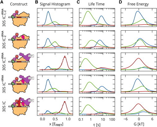
smFRET study of IF3 conformational dynamics on the 30S initiation complex of the bacterial ribosome. (A) Schematic illustrations of experimental contsructs 30S ${\text{IC}}_{-1,-2}^{-\text{tRNA}}$, 30S ${\text{IC}}_{-2}^{-\text{tRNA}}$, 30S ${\text{IC}}_{-1}^{-\text{tRNA}}$, 30S ${\text{IC}}^{-\text{tRNA}}$, and 30S IC^fMet. (B) Per-state observation histograms. (C) Lifetime distributions. (D) Free-energy distributions. States 1–3 are represented by blue, green, and red lines, respectively. To see this figure in color, go online.

Previous analysis was performed with the vbFRET software (15) that obtains VB estimates for each individual $E_{\text{FRET}}$ trajectory. In this particular set of experiments, most trajectories are static (i.e., no conformational transitions are observed before the fluorophores photobleach). This makes it more difficult to distinguish between intermediate and extended or compact states, since within individual trajectories, there are few transitions that reveal the location of a state relative to others. For this reason, the resulting $E_{\text{FRET}}$ means of states in each trajectory were assigned to three empirically chosen bins with intervals (0,0.3), (0.3,0.7), and (0.7,1.0), where all potential intermediate states were grouped into the middle interval. The compact state was found to be highly populated in a correctly assembled 30S IC, whereas the extended state is highly populated in incorrectly assembled or incomplete 30S ICs, which either lack IFs, lack fMet-tRNA^fMet, contain an incorrect elongator aminoacyl-tRNA, or contain an incorrect near-start codon (29).

In our analysis, we first performed EB inference on the aggregate data from five experiments that were recorded under different conditions: 30S ${\text{IC}}_{-1,-2}^{-\text{tRNA}}$ (lacking IF1, IF2, and tRNA), 30S ${\text{IC}}_{-2}^{-\text{tRNA}}$ (lacking IF2 and tRNA), 30S ${\text{IC}}_{-1}^{-\text{tRNA}}$ (lacking IF1 and tRNA), 30S ${\text{IC}}^{-\text{tRNA}}$ (lacking tRNA), and 30S IC^fMet (a correctly assembled 30S IC). This aggregate dataset contained 4233 trajectories with $4.0\cdot {10}^5$ total data points. Three states were used to facilitate comparison with the previous results based on VB analysis. After inference, separate parameter distributions were estimated from the sufficient statistics of each individual experiment, as described in Eq. 9. The results of this analysis, which does not require that the user manually assign the $E_{\text{FRET}}$ means of states in each trajectory to empirically chosen bins, are in excellent agreement with previous results based on explicitly defined bin intervals. Fig. 2 shows observation histograms for each state, as well as distributions of the lifetime and free energy of each state relative to the other states (see section S5 of the Supporting Material for the definitions of these quantities). The width of each distribution provides us with a confidence interval on each of the parameters. The fractional occupancies obtained for each experiment (Table 1) similarly show a close correspondence to the values obtained with the VB-based results.

Table 1.

Relative occupancies of IF3 states obtained from VB and EB- analysis of labeled subpopulations

Construct	VB + binning			EB
	ext.	int.	cpt.	ext.	int.	cpt.
30S ${\text{IC}}_{-1,-2}^{-\text{tRNA}}$	0.54	0.40	0.06	0.63	0.30	0.07
30S ${\text{IC}}_{-2}^{-\text{tRNA}}$	0.52	0.45	0.03	0.47	0.43	0.10
30S ${\text{IC}}_{-1}^{-\text{tRNA}}$	0.23	0.11	0.66	0.14	0.15	0.72
30S ${\text{IC}}^{-\text{tRNA}}$	0.56	0.42	0.02	0.60	0.34	0.06
30S ICfMet	0.15	0.17	0.68	0.15	0.21	0.64

Relative occupancies of the extended (ext.), intermediate (int.), and compact (cpt.) conformations of IF3, obtained from binned analysis with vbFRET (29) and EB-based analysis of labeled subpopulations.

Unlabeled subpopulations: the influence of EF-G binding on the GS1-GS2 equilibrium

We now demonstrate that the extended EB estimation procedure described by Eq. 14 can be used to identify kinetically distinct subpopulations of states and estimate the transition rates for each subpopulation of states. As an example of this use case, we perform analysis of a set of smFRET experiments investigating the role of elongation factor (EF) G, a member of the GTPase family of translation factors, during translation elongation.

After the addition of each amino acid to the nascent polypeptide chain during translation elongation, EF-G binds to the ribosomal pretranlsocaiton (PRE) complex and hydrolyzes one molecule of GTP as it promotes the movement of the ribosome along the mRNA by precisely one triplet-nucleotide codon, a process termed translocation (Fig. 3 A). The overall process of translocation can be broken up into three smaller multistep processes. The first of these is a thermally driven, reversible transition between two global states (denoted as GS1 and GS2) of the PRE complex. The overall process of translocation can be broken up into three smaller multistep processes. This conformational transition is followed by binding of EF-G to the PRE complex, resulting in a transient stabilization of the GS2 state of the PRE complex that is long enough to enable the third step, a GTP hydrolysis-driven movement of the ribosome along the mRNA. The effect that binding of EF-G has on the dynamic equilibrium between the GS1 and GS2 states of the PRE complex can be studied using smFRET by labeling two ribosomal structural elements with a FRET donor-acceptor pair and substituting GTP with a nonhydrolyzable analog (GDPNP) that prevents GTP hydrolysis and the associated movement of the ribosome along its mRNA template.

Figure 3.

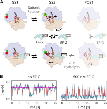
smFRET experiments (31) measuring the influence of EF-G on the GS1-GS2 equilibrium in the bacterial ribosome. (A) The kinetic pathway for translocation is believed to have three steps: a reversible rotation of the two subunits (purple and orange), followed by the binding of EF-G (green), which stabilizes the rotated GS2 state long enough for a GTP-driven transition to the posttranslocation (POST) complex, blocked here by substitution of GTP by a nonhydrolyzable analog. (B) smFRET signals reporting on the GS1-GS2 transition show a shift of the equilibrium from the GS1 state (magenta line) toward the GS2 state (cyan line) in the presence of EF-G. To see this figure in color, go online.

Fig. 3 B shows two $E_{\text{FRET}}$ trajectories that exhibit thermally driven, reversible transitions between GS1 and GS2. The first trajectory is from an experiment that was recorded in the absence of EF-G and shows a preference for the GS1 state. The second trajectory, from an experiment that was recorded in the presence of 500 nM EF-G and 1 mM GDPNP, shows a dramatic shift of the equilibrium toward the GS2 state. Qualitative comparison of these two trajectories suggests that EF-G destabilizes the GS1 state and stabilizes the GS2 state in the subpopulation of EF-G-bound PRE complexes. To quantify this difference in transition rates and characterize its dependence on EF-G concentration, we must obtain separate estimates for the distribution on transition rates for the EF-G-free and EF-G-bound subpopulations of PRE complexes in an experiment.

EB analysis of a series of experiments performed at increasing EF-G concentrations is shown in Fig. 4. As with the previous experiment we first analyze the aggregate data to identify two states. The aggregate data for seven different EF-G concentrations contained 2472 trajectories with 2.3 × 10⁵ total data points. As can be seen in the observation histograms (Fig. 4 A), the occupancy of the GS2 state (cyan line) increases with the EF-G concentration. Conventional EB analysis with a single population (Fig. 4 B) naturally reveals a bimodal signature in the posterior (solid lines) that hints at the existence of two (unlabeled) subpopulations. This signature is absent from the prior (dashed lines), since EB analysis assumes all transition probabilities are governed by the same prior distribution. Because a very limited number of transitions between GS1 and GS2 can be observed in any one signal trajectory before one of the fluorophores photobleaches, it is not possible to obtain a precise estimate of the transition rates for each individual PRE complex. As a result, the two peaks in Fig. 4 B have a very high degree of overlap, showing that it would be difficult to determine the population membership for each signal trajectory using any form of binning approach. This ambiguity of subpopulation membership is greatly reduced when using the subpopulation analysis technique described in the previous section (see also Section S4.5 of the Supporting Material), which produces two much-better-resolved peaks (Fig. 4 C). Table 2 lists the population fraction and free energy difference obtained from EB estimation with unlabeled subpopulations. As should be expected, the relative size of the EF-G-bound subpopulation increases as the concentration of EF-G increases.

Figure 4.

Analysis of GS1-GS2 equilibrium as a function of EF-G concentration. (A) Histogram of aggregate measurements, split by GS1 (magenta line) and GS2 (cyan line) states. (B) EB prior (dashed line) and mean posterior (solid line) on the free-energy difference $\text{Δ}G=G_{\text{GS}1}-G_{\text{GS}2}$. A bimodal signature in the posterior is visible in experiments where EF-G is present. (C) Prior and posterior after unlabeled subpopulation analysis, showing an increasing occupancy of the bound fraction (orange line) relative to the nonbound fraction (green line) as a function of EF-G concentration. To see this figure in color, go online.

Table 2.

EF-G concentration dependence in unlabeled subpopulation analysis of GS1-GS2 equilibrium

EF-G	0 nM	5 nM	50 nM	500 nM	1000 nM
${\rho }_{+\text{EF}-\text{G}}$	0.13	0.30	0.56	0.65	0.67
$\text{Δ}{G}_{+\text{EF}-\text{G}}$	1.7	1.2	1.3	1.4	1.4
$\text{Δ}{G}_{-\text{EF}-\text{G}}$	−2.4	−1.7	−0.8	−0.4	−0.4

Fraction of EF-G bound complexes, ${\rho }_{+\text{EF}-\text{G}}$, and the free energy difference between the GS1 and GS2 state, $\text{Δ}G$, for the bound and unbound subpopulation, as a function of EF-G concentration.

Model selection

One of the stated advantages of the VB and EB methods is that they optimize a lower bound for the log evidence, a quantity that may be used to decide among analysis results with different numbers of states. Previous benchmarks using computer-simulated data have shown that EB estimation systematically outperforms VB and ML methods in model-selection tasks (25). Not only does EB estimation more accurately determine the number of states in individual trajectories, preventing both under- and overfitting, but the method can also determine the correct number of states starting from a larger number of candidate states, leaving superfluous states unpopulated.

In practice, experimental data differ from simulated data in that they are never in precise agreement with a given statistical model. In smFRET experiments, for example, we assume a Gaussian distribution of $E_{\text{FRET}}$ values for each state. With one exception (17), all HMM approaches for analysis of (time-binned) smFRET data make this same assumption (14–16,18). In reality, however, the $E_{\text{FRET}}$ value exhibits a sigmoidal dependence on the distance between the fluorophores, resulting in a distribution of $E_{\text{FRET}}$ values that is skewed toward the middle of the spectrum and exhibits a subtle, but systematic, deviation from the idealized Gaussian shape assumed in the model. Distributions of $E_{\text{FRET}}$ values further show heavy tails that likely arise from artifacts such as intermittent photoblinking of fluorophores (32), incorrect detection of the photobleaching transition, and errors in determining the background fluorescence intensity of individual trajectories.

In general, systematic discrepancies and artifacts can cause a statistical algorithm to correct for the fact that observed measurement values are not precisely distributed according to the assumed model by populating additional states, as was found to be the case in our initial analysis of experimental data (25). In Fig. 5, we revisit this notion by examining results obtained by estimating models with 2–10 states on the same two data sets that were analyzed in the previous sections. As in previous work (25), we calculate an effective number of states, $K_{\text{eff}}=\text{exp}\left[-{\sum }_{k=1}^K{\zeta }_k\log {\zeta }_k\right]$, in terms of ${\zeta }_k={\sum }_n{\text{Γ}}_{nk}/{\sum }_{nk}{\text{Γ}}_{nk}$, the fraction of time points assigned to each state. When performing analysis on simulated data, there is typically a range of solutions for different K that yield the same (correct) $K_{\text{eff}}$ value and leave any additional states empty (25). Consistent with our previous study (25), the results in Fig. 5 A show that $K_{\text{eff}}$ steadily increases with the number of candidate states, and it is not clear that there is an optimum $K_{\text{eff}}$ value beyond which the lower bound, L, decreases. In other words, the fit of experimental data to the model can be improved by adding incremental low-occupancy states that capture outliers in the data, even when using model-selection criteria. This is undesirable behavior, as such outlier states are more likely to be indicative of measurement artifacts than of actual conformational states of interest. However, it is important to note that this behavior is different from the typical overfitting that is associated with ML estimation. ML methods obtain a better fit by assigning natural statistical variations to separate states, and will do so even for simulated data that is in perfect agreement with the hypothesized model. EB analysis generally obtains the correct result on simulated data but uncovers unnatural variations in experimental data that are real from a statistical point of view but do not contain useful information about actual conformational transitions.

Figure 5.

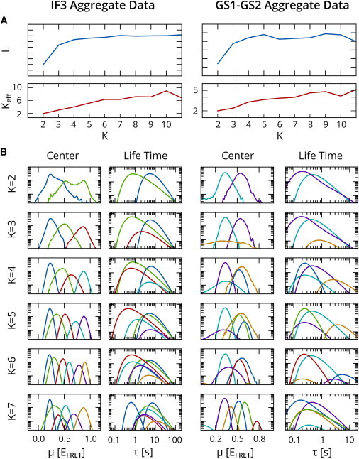
EB analysis of IF3 and GS1-GS2 aggregate data for an increasing number of states, K. (A) Evidence lower bound L and effective number of populated states, K_eff, as a function of K. (B) Averaged posterior on state centers, μ, and lifetimes, τ. To see this figure in color, go online.

Examples of these systematic discrepancies can be seen in Fig. 5 B, which shows the averaged posterior distribution on the state centers, ${\mu }_{nk}$, and state dwell times, ${\tau }_{nk}$, obtained by analyzing the aggregate data sets from the previous sections with increasing number of states. When plotted on a logarithmic scale, a Gaussian distribution will have a parabolic shape. The curves for ${\mu }_{nk}$ clearly show both asymmetries and aberrant tails that deviate from this idealized form. As a result, it is generally difficult to say whether too many states are used, since the curves obtained at higher K do show a closer agreement with the shape assumed in the model.

For this reason, we suggest that users do not indiscriminately rely on the lower bound for model selection; thus, some prudent decision-making with regard to model selection may still be required on the part of the experimentalist. One rule of thumb is to treat states observed in <5% of the trajectories with some caution. Additional states may simply 1), capture artifacts, such as intermediate points between a transition (15); 2), split a single state into a short-lived and long-lived variant (which may mean that a subpopulation as described in Methods is necessary); or 3), isolate the non-Gaussian tails of actual states. Moreover, any decreases in the lower bound indicate that the method has converged to a local maximum rather than the globally optimal result, since adding an empty state to the previous result should result in the same, larger L value. In this case, the user may either opt to perform additional restarts with random initializations of ${\psi }_0$, to make it more likely that the global optimum is found for each number of candidate states, or accept the point where L begins to decrease as a bound on the number of states that can be confidently inferred, given computational limitations. As an example, the GS1/GS2 experiment shows a decrease in L at $K=6$, whereas the lifetime plot for the blue state falls off the scale at $K=5$, suggesting that $K=4$ is the largest number of states that is credible. Also note that these four states form two pairs with similar $E_{\text{FRET}}$ values but different lifetimes, which is consistent with our knowledge that this experiment in fact does contain kinetically distinct subpopulations. Finally, we note that the conformational trajectory can be inferred with more confidence when more transitions are observed, as it allows the inference procedure to more confidently situate one state relative to others. In cases such as the IF3/30S IC experiment, where the majority of trajectories do not exhibit transitions, analysis results could be improved by shuttering the excitation source to, optimally, obtain a state lifetime of the order of 10 time points.

In summary, although EB methods provide model-selection criteria that are superior to those employed in ML and VB estimation (when applied to computer-simulated data), a methodological caveat in any statistical analysis is that model-selection criteria are only as accurate as the representation of the measurement data in the model. We emphasize that this limitation is by no means unique to EB analysis. ML and VB approaches typically use precisely the same Gaussian distribution of measurement values and suffer from the same defects. It is merely the case that these issues are obfuscated when signal trajectories are analyzed individually, since an individual signal trajectory rarely contains enough data points to make discrepancies between the data and the model apparent, and the experimentalist makes a judgment call as to how many conformational states they think are required as part of the data inference postprocessing. The advantage of the EB methodology is that analyzing all trajectories at once allows us to identify systematic deviations between data and model, allowing us to assess whether there is sufficient agreement between the data and the model for model-selection criteria to be effective.

Discussion

Although HMMs have proven an immensely popular and effective tool for inferring states and transition rates from individual signal trajectories, combining results from the analysis of multiple trajectories has remained a difficult task. Typically, users manually specify a set of bin intervals, as was done in our previous, VB-based analysis of the IF3 data (29), that allow states identified in individual signal trajectories to be clustered according to their inferred parameter values. In contrast, the EB method uniquely enables simultaneous inference on multiple signal trajectories in a statistically robust manner that eliminates the need for user-defined bin intervals and is consequently less prone to user bias.

By exploiting the advantages of simultaneously analyzing multiple $E_{\text{FRET}}$ trajectories using the EB method, we have developed estimation procedures that uniquely enable us to automate widely encountered tasks in the analysis of smFRET experiments. The first of these tasks is exemplified by our analysis of the IF3 experiments, which demonstrates how $E_{\text{FRET}}$ trajectories from a large number of experiments recorded under different experimental conditions can first be simultaneously analyzed to identify a common set of states and then be subsequently reanalyzed to calculate a separate prior distribution for each experiment, allowing characterization of how the state occupancies and transition rates vary between experiments. The second task is exemplified by our analysis of the GS1/GS2 experiments, which demonstrates how the simultaneous analysis of an entire population of $E_{\text{FRET}}$ trajectories can be used to automatically identify and characterize subpopulations of molecules occupying functionally and/or conformationally distinct states that exhibit similar $E_{\text{FRET}}$ values but differ in the rates of transitions between states.

For each set of experiments, the results of the EB-based analysis are largely consistent with previous results based on VB methods. However, although the previous VB-based analysis required the use of experiment-specific postprocessing procedures that are time-consuming to implement, subject to user bias, and difficult to validate, our EB method can be used to obtain results rapidly and with little to no manual intervention by the user. Moreover, the EB approach optimizes a well-defined, statistical, model-selection criterion, the lower bound for the log evidence, which in principle can be used to compare and decide among different analyses of the same data.

Our EB-based analysis of smFRET data also demonstrates that comparing the prior and posterior distributions can often provide useful qualitative diagnostics that indicate whether a given model is appropriate for the data. In the case of the GS1/GS2 experiments, for example, we are able to calculate a posterior distribution on the free-energy difference between states that reveals a systematic mismatch between the single population of PRE complexes that is assumed in conventional EB analysis and the two subpopulations of PRE complexes that are actually present in the experiment (i.e., EF-G-free and EF-G-bound). This mismatch is resolved when we extend our EB method to identify the two subpopulations within the set of multiple $E_{\text{FRET}}$ trajectories. In a similar way, combining results from multiple trajectories using our EB method allows us to see that the distribution of $E_{\text{FRET}}$ values associated with a given conformational state often exhibits heavy tails and is skewed relative to the Gaussian distribution that is typically assumed in HMM analyses of smFRET data. Whereas discrepancies between the data and the statistical model will always exist, they are much more difficult to detect in individual trajectories (e.g., in ML- and VB-based HMM analyses of smFRET data). An important advantage of the EB method, therefore, is that it can tease out such discrepancies, which inform us as to how our assumptions about the data need to be adjusted in the next iteration of statistical model design.

We conclude by noting that the EB estimation framework is applicable to a wide range of single-molecule techniques. Although here we have analyzed smFRET experiments exclusively, our approach is by no means restricted to this platform. Adaptation of the EB algorithm presented here to the analysis of optical trapping and magnetic tweezers experimental data is possible with minimal modifications and we have recently collaborated to adapt the EB algorithm presented here to the analysis of tethered particle motion experiments (33).

References

- 1.Tinoco I., Jr., Gonzalez R.L., Jr. Biological mechanisms, one molecule at a time. Genes Dev. 2011;25:1205–1231. doi: 10.1101/gad.2050011. [DOI] [PMC free article] [PubMed] [Google Scholar]
- 2.Joo C., Balci H., Ha T. Advances in single-molecule fluorescence methods for molecular biology. Annu. Rev. Biochem. 2008;77:51–76. doi: 10.1146/annurev.biochem.77.070606.101543. [DOI] [PubMed] [Google Scholar]
- 3.Borgia A., Williams P.M., Clarke J. Single-molecule studies of protein folding. Annu. Rev. Biochem. 2008;77:101–125. doi: 10.1146/annurev.biochem.77.060706.093102. [DOI] [PubMed] [Google Scholar]
- 4.Neuman K.C., Nagy A. Single-molecule force spectroscopy: optical tweezers, magnetic tweezers and atomic force microscopy. Nat. Methods. 2008;5:491–505. doi: 10.1038/nmeth.1218. [DOI] [PMC free article] [PubMed] [Google Scholar]
- 5.Cornish P.V., Ha T. A survey of single-molecule techniques in chemical biology. ACS Chem. Biol. 2007;2:53–61. doi: 10.1021/cb600342a. [DOI] [PubMed] [Google Scholar]
- 6.Rabiner L. A tutorial on hidden Markov models and selected applications in speech recognition. Proc. IEEE. 1989;77:257–286. [Google Scholar]
- 7.Eddy S.R. Hidden Markov models. Curr. Opin. Struct. Biol. 1996;6:361–365. doi: 10.1016/s0959-440x(96)80056-x. [DOI] [PubMed] [Google Scholar]
- 8.Bilmes, J. 1998. A Gentle Tutorial of the EM Algorithm and its Application to Parameter Estimation for Gaussian Mixture and Hidden Markov Models. Technical Report, University of California Berkeley, ICSI-TR-97-021.
- 9.Chung S.H., Moore J.B., Gage P.W. Characterization of single channel currents using digital signal processing techniques based on Hidden Markov Models. Philos. Trans. R. Soc. Lond. B Biol. Sci. 1990;329:265–285. doi: 10.1098/rstb.1990.0170. [DOI] [PubMed] [Google Scholar]
- 10.Qin F., Auerbach A., Sachs F. Maximum likelihood estimation of aggregated Markov processes. Proc. Biol. Sci. 1997;264:375–383. doi: 10.1098/rspb.1997.0054. [DOI] [PMC free article] [PubMed] [Google Scholar]
- 11.Qin F., Auerbach A., Sachs F. A direct optimization approach to hidden Markov modeling for single channel kinetics. Biophys. J. 2000;79:1915–1927. doi: 10.1016/S0006-3495(00)76441-1. [DOI] [PMC free article] [PubMed] [Google Scholar]
- 12.Smith D.A., Simmons R.M. Models of motor-assisted transport of intracellular particles. Biophys. J. 2001;80:45–68. doi: 10.1016/S0006-3495(01)75994-2. [DOI] [PMC free article] [PubMed] [Google Scholar]
- 13.Kruithof M., van Noort J. Hidden Markov analysis of nucleosome unwrapping under force. Biophys. J. 2009;96:3708–3715. doi: 10.1016/j.bpj.2009.01.048. [DOI] [PMC free article] [PubMed] [Google Scholar]
- 14.McKinney S.A., Joo C., Ha T. Analysis of single-molecule FRET trajectories using hidden Markov modeling. Biophys. J. 2006;91:1941–1951. doi: 10.1529/biophysj.106.082487. [DOI] [PMC free article] [PubMed] [Google Scholar]
- 15.Bronson J.E., Fei J., Wiggins C.H. Learning rates and states from biophysical time series: a Bayesian approach to model selection and single-molecule FRET data. Biophys. J. 2009;97:3196–3205. doi: 10.1016/j.bpj.2009.09.031. [DOI] [PMC free article] [PubMed] [Google Scholar]
- 16.Bronson J.E., Hofman J.M., Wiggins C.H. Graphical models for inferring single molecule dynamics. BMC Bioinformatics. 2010;11(Suppl 8):S2. doi: 10.1186/1471-2105-11-S8-S2. [DOI] [PMC free article] [PubMed] [Google Scholar]
- 17.Liu Y., Park J., Ha T. A comparative study of multivariate and univariate hidden Markov modelings in time-binned single-molecule FRET data analysis. J. Phys. Chem. B. 2010;114:5386–5403. doi: 10.1021/jp9057669. [DOI] [PubMed] [Google Scholar]
- 18.Greenfeld M., Pavlichin D.S., Herschlag D. Single Molecule Analysis Research Tool (SMART): an integrated approach for analyzing single molecule data. PLoS ONE. 2012;7:e30024. doi: 10.1371/journal.pone.0030024. [DOI] [PMC free article] [PubMed] [Google Scholar]
- 19.Okamoto K., Sako Y. Variational Bayes analysis of a photon-based hidden Markov model for single-molecule FRET trajectories. Biophys. J. 2012;103:1315–1324. doi: 10.1016/j.bpj.2012.07.047. [DOI] [PMC free article] [PubMed] [Google Scholar]
- 20.Dempster A., Laird N., Rubin D. Maximum likelihood from incomplete data via the EM algorithm. J. R. Stat. Soc. Series B Stat. Methodol. 1977;39:1–38. [Google Scholar]
- 21.Baum L., Petrie T., Weiss N. A maximization technique occurring in the statistical analysis of probabilistic functions of Markov chains. Ann. Math. Stat. 1970;41:164–171. [Google Scholar]
- 22.Jordan M., Ghahramani Z., Jaakkola T. An introduction to variational methods for graphical models. Mach. Learn. 1999;233:183–233. [Google Scholar]
- 23.Berger J. Bayesian robustness and the Stein effect. J. Am. Stat. Assoc. 1982;77:358–368. [Google Scholar]
- 24.Kass R., Steffey D. Approximate Bayesian inference in conditionally independent hierarchical models (parametric empirical Bayes models) J. Am. Stat. Assoc. 1989;84:717–726. [Google Scholar]
- 25.van de Meent J.-W., Bronson J.E., Wiggins C.H. Hierarchically-coupled hidden Markov models for learning kinetic rates from single-molecule data. Proc. Int. Conf. Mach. Learn. 2013;28:361–369. [PMC free article] [PubMed] [Google Scholar]
- 26.Blanco M., Walter N.G. Analysis of complex single-molecule FRET time trajectories. Methods Enzymol. 2010;472:153–178. doi: 10.1016/S0076-6879(10)72011-5. [DOI] [PMC free article] [PubMed] [Google Scholar]
- 27.Bishop C.M. Springer; New York: 2006. Pattern recognition and machine learning. [Google Scholar]
- 28.Reference deleted in proof.
- 29.Elvekrog M.M., Gonzalez R.L., Jr. Conformational selection of translation initiation factor 3 signals proper substrate selection. Nat. Struct. Mol. Biol. 2013;20:628–633. doi: 10.1038/nsmb.2554. [DOI] [PMC free article] [PubMed] [Google Scholar]
- 30.Laursen B.S., Sørensen H.P., Sperling-Petersen H.U. Initiation of protein synthesis in bacteria. Microbiol. Mol. Biol. Rev. 2005;69:101–123. doi: 10.1128/MMBR.69.1.101-123.2005. [DOI] [PMC free article] [PubMed] [Google Scholar]
- 31.Fei J., Bronson J.E., Gonzalez R.L., Jr. Allosteric collaboration between elongation factor G and the ribosomal L1 stalk directs tRNA movements during translation. Proc. Natl. Acad. Sci. USA. 2009;106:15702–15707. doi: 10.1073/pnas.0908077106. [DOI] [PMC free article] [PubMed] [Google Scholar]
- 32.Blanchard S.C., Gonzalez R.L., Puglisi J.D. tRNA selection and kinetic proofreading in translation. Nat. Struct. Mol. Biol. 2004;11:1008–1014. doi: 10.1038/nsmb831. [DOI] [PubMed] [Google Scholar]
- 33.Johnson, S., J.-W. van de Meent, C. H. Wiggins, R. Phillips, and M. Lindén. Multiple Lac-mediated loops revealed by Bayesian statistics and tethered particle motion. Preprint, submitted February 4, 2014. arXiv. http://arxiv.org/abs/1402.0894v1. [DOI] [PMC free article] [PubMed]
Associated Data
This section collects any data citations, data availability statements, or supplementary materials included in this article.