

Abstract
We have often observed unexpected state transitions of complex systems. We are thus interested in how to steer a complex system from an unexpected state to a desired state. Here we introduce the concept of transittability of complex networks, and derive a new sufficient and necessary condition for state transittability which can be efficiently verified. We define the steering kernel as a minimal set of steering nodes to which control signals must directly be applied for transition between two specific states of a network, and propose a graph-theoretic algorithm to identify the steering kernel of a network for transition between two specific states. We applied our algorithm to 27 real complex networks, finding that sizes of steering kernels required for transittability are much less than those for complete controllability. Furthermore, applications to regulatory biomolecular networks not only validated our method but also identified the steering kernel for their phenotype transitions.
Many complex systems of scientific interest can be represented as directed networks in which a set of nodes are connected in pairs by directed edges or arcs1,2,3,4,5,6,7,8,9,10. Because of the interactions among nodes in a network, perturbing some nodes can affect other nodes, which may cause the state transition of a network. In reality, we have often observed some unexpected state transitions of a complex system (for example, from a normal sate to an abnormal state)11,12. Here we are interested in how to effectively steer the system from an unexpected state to a desired state by applying suitable input control signals. The main purpose of this work is to provide a theoretical framework that addresses such an issue for complex networks, especially, regulatory biomolecular networks.
A regulatory biomolecular network is orchestrated by the interactions of many molecules in a cell13,14. A living cell should stay at a normal (at least, healthy) phenotype. However, by some unknown perturbation or stimuli, a regulatory biomolecular network can be transited from a normal phenotype to a disease phenotype. It thus is desirable to steer the regulatory network to transit from the abnormal phenotype to a healthy phenotype. To study the phenotype transitions, a regulatory biomolecular network is represented by a directed network in which molecules are represented by nodes and the interactions between molecules are represented by arcs2,3,4,5,6,15,16,17. As a result, cellular phenotypes can be defined by the network states that represent all the molecular expressions in the network collectively while a phenotypic change or cellular behavior change can be described as a dynamic transition between two states of the network, such as a complex disease progression11,12, p53-mediated DNA damage response network18, T helper cells differentiation19, and epithelial to mesenchymal transition20.
The empirical studies in the cellular reprogramming field have indicated that one phenotype can be transited to another by overexpressing a few transcription factors21,22,23,24,25,26 (steering nodes). In the field of the network-based methodologies for drug designs2,6,17, trial-and-error-based methods according to the researcher's experiences have found that a few drug targets are enough to achieve a transition from a disease state to a healthy state for many complex diseases15,17. For example, acute promyelocytic leukemia (APL), a subtype of acute myeloid leukemia (AML), has been successfully treated with therapy which utilizes all-trans-retinoic acid (ATRA). However, among patients with non-APL AML, ATRA-based treatment has not been effective. Based on the literature and experimental verifications, Schenk et al27 have concluded that ATRA plus tranylcypromine (TCP) can effectively treat non-APL AML. From the viewpoint of dynamic systems control theory, the cellular network in charge of APL AML cell line can be transited from the abnormal state to a healthy state through the targets of ATRA while the cellular network in charge of non-APL AML cell line cannot be transited from the abnormal state to a healthy state through only the targets of ATRA. However, current researches in these fields have little or no control theory involved although control theory has been successfully applied to study the state transition of engineering systems.
Although the concept of controllability of dynamic linear systems28 can be applied to complex networks29, most of their parameters are either unknown or known only approximately and are time dependent7. In addition, even if all the parameters are available, the determination of controllability is computationally prohibitive even for moderate-size networks. Nevertheless, Liu, et al7 have recently applied the concept of structural controllability30,31,32 to study the controllability of directed complex networks, and derived the theoretical result of complete controllability, i.e., the transition between any two states of a network (rather than two specific states). According to their result, the minimum number of driver nodes is 80% of nodes in a regulatory biomolecular network in order to have complete controllability, which seems to contradict some empirical findings in cellular reprogramming field33. In order to reduce the number of driver nodes, Nepusz and Vicsek8 have studied the complete controllability of complex networks in terms of edge dynamics instead of node dynamics. In addition, with a strong assumption that each driver node can control its outgoing edges independently7,8,9, Nacher and Akutsu have studied the complete controllability of bipartite networks9. In fact, a phenotype can be considered as a high-dimensional attractor of the complex network34. The transition between two specific phenotypes (rather than any two phenotypes) stems from the change of states of some (not all) nodes in a subspace of the full state space35. In addition, complete controllability often requires more steering nodes and affects the full state space in the network (Figure 1b). Therefore, it is asking for too much to have complete controllability in studying the transition between two specific states.
Figure 1. Illustration of network transittability.

(a) Considering the transittability of the network between two specific states x0 and x1 as shown here and finding the steering kernel for such a state transition. Nodes with the same color at two states (e.g., v4, v5, v6) indicates that they are unchanged while nodes with different colors (e.g., v2, v1, v3) indicates that they are unchanged at two states. “*” in the structure matrix A of the network represents the free parameters while “0” represents the fixed parameters. “*” in two states x0 and x1 represents the value of corresponding nodes different while “0” represents the value of corresponding nodes indifferent at two states. (b) From the concept of complete controllability, two input control signals should be directly applied to two steering nodes v6 and v5 to transit the network between any two states, including two specific states x0 and x1. One can see that (1) more steering nodes than necessary are needed and (2) the full state space with six dimensions is affected for such a state transition, which may cause side effects. (c) From our new concept of transittability and new theorems, only one steering node v3 is needed for the transition between two specific states x0 and x1. (d) This is the traditional sufficient and necessary condition for transittability of two specific states x0 and x1 which is actually intractable. (e) Using our new sufficient and necessary condition for transittability of two specific states x0 and x1, we can identify the steering kernel by solving an optimal assignment of weighted bipartite graphs via an efficient graph-theoretic algorithm.
Differently from complete controllability between any two states, here we aim to develop a theoretic framework for studying transitions between two specific states of directed complex networks by introducing a new concept of transittability, and further apply our theoretical results for identifying the steering kernels of 27 real complex networks and 4 biomolecular networks. Here, “real complex networks” mean that the networks are constructed based on mathematical models of real systems. Specifically, we first define the concepts of transittability of a complex directed network and develop a new sufficient and necessary condition for transittability under which a specific structural state of a complex network can be transited to another. Our new condition can be efficiently verified by a graph-theoretic algorithm. We call a node on which an input control signal is directly acted as a steering node. We then define the steering kernel as a minimal set of steering nodes to steer the network to transit from one state to another. Here we stress that the steering kernel is different from the minimum set of driver nodes in the paper7. As illustrated in Supplementary Information I, we show that a network cannot be guaranteed to transit from one specific state to any other state by acting only on the minimum set of driver nodes identified by the minimum input theorem7, whereas the steering kernel defined in this work can ensure such a transition. Furthermore, we develop a graph-theoretic algorithm to identify the steering kernel for transition between two specific states. We apply our algorithm to 27 real complex networks, finding that the minimum numbers of steering nodes required for transittability are much less than those for complete controllability. In addition, we also apply our algorithms to several real biomolecular networks, finding that not only is the number of the identified steering nodes for cellular phenotype transitions small, but also the identified steering nodes are consistent with empirical findings in the literature.
Results
Transittability
Although most complex dynamic systems are nonlinear, the controllability of nonlinear systems is in many aspects structurally similar to that of linear systems7,36,37. Actually, to ultimately develop the control strategies for complex nonlinear networks, a necessary and fundamental step is to investigate the controllability (especially structural controllability) of complex networks with linear dynamics. In this study, we thus consider the linear time-invariant nodal dynamics of a complex network with n nodes, where the activity of node i, xi(t), can be described by the following equations
 |
where aij ≠ 0 if node j directly affects node i, that is, there is an arc from node j to node i in the network, and otherwise aij = 0. σi = 1 if input control signal ui(t) directly acts on node i and otherwise σi = 0. In this study, we are interested not in the complete controllability7, but in the transittability of the system (1), which concerns the transition between two specific states by a suitable choice of input control signals (Figure 1c). Formally, the system (1) is said to be transittable between two given specific states x0 and x1 if it can be transited between x0 and x1 in finite time tf by proper input control signals u(t) ( ). Note that the system (1) is transittable between any two states by simply acting one independent input control signal on each of n nodes. That is, all nodes are steering nodes, then we have σi = 1 for i = 1,2,…,n and thus
  . However in this study we are interested in finding the minimum set of steering nodes (called steering kernel) to achieve the state transition between two specific states, in other worlds, minimizing
  while the system (1) is transittable between two given specific states x0 and x1.
The system (1) can be rewritten in the vector-matrix format as follows
 |
where the n-dimensional vector x(t) = (x1(t), …, xn(t))T represents the state of the network with n nodes at time t. The n × n matrix A = (aij) describes the interaction relationship and strength between nodes. The n × p matrix B is called the input control matrix that corresponds to the steering nodes. The p-dimensional vector u(t) = (u1(t), …, up(t))T represents the input control signals. As in many situations10,21,22,23,24,25,26, one controller cannot produce multiple independent input control signals. Here we assume that one controller can produce only one independent input control signal. Therefore, all elements in the j-th column of matrix B are all zeroes except for the s-th element if the j-th input control signal directly acts on node s. Our theoretical result (Supplementary Information Section II) shows that the system (2) is transittable between states x0 and x1 if and only if there exists a positive number tf such that
 |
 |
where span(C) represents the subspace spanned by the column vectors of matrix C and is called the controllable subspace. Now finding the steering kernel to steer the system (2) from state x0 to x1 can be formulated as a problem to find the matrix B with the minimum number of columns such that condition (3) is true. However, the calculation of either  is complicated and condition (3) is computationally intractable (Figure 1d). Next, we state our first key result, i.e., we prove (see Supplementary Information Section II) that the system (2) is transittable between two specific states x0 and x1 with either belonging to span(C) if and only if
 |
 |
where  . The transittability is typically considered between two stable states or one stable state and another state. Let us say that x1 is a stable state, we can always assume that x1 = 0 (the origin) without loss of generality, i.e., we can replace x0 with x0 – x1 if x1 ≠ 0, which does not affect the result. Then we have that the system (2) is transittable between a specific states x0 and the origin if and only if
 |
 |
where B0 = [x0, B]. Although the condition (7) is much easier to be verified than the condition (3), the calculation of either rank(C0) or rank(C0) is still prohibitive because of the large size n of a complex network, the uncertainty, time dependence of the entries in matrices A and/or vector x0. Note that the transittability is not only to control a state to the origin, but also to control a state from the origin to other specific states.
Identifying the steering kernel
To overcome the computational impedance in verifying condition (7), we further introduce the structural transittability via the concepts of structural matrix and generic dimension of controllable subspace. M is said to be a structural matrix if its entries are either fixed zeros or independent free parameters.  is called admissible (with respect to M) if it can be obtained by fixing the free parameters of M at some specific values. If A and B are structural matrices, system (2) is called a structural system and is denoted by (A, B). Associated with a structural system (A, B), a directed graph G(A, B) = (V, E) can be defined with the set of nodes V = VAUVB, where VA = {x1,…, xn}: = {v1,…, vn} is the set of state vertices, corresponding to the n state components while VB = {u1,…, up}: = {vn+1,…, vn+p} is the set of input vertices, corresponding to the p inputs, and the set of arcs E = EAUEB, where EA = {(xj, xi) = (vj, vi) | aij ≠ 0} is the set of directed edges between state vertices while EB = {(uj, xi) = (vn+j, vi) | bij ≠ 0} is the set of directed edges between input vertices and state vertices. We can also define a directed network G(A) = (VA, EA) with respect to a structural matrix A (Figure 1a). In a directed graph, an elementary path is a sequence of arcs
  where all vertices {vi0, vi1, …, vik} are different, and when vi0 = vik, it is called an elementary cycle. A stem is an elementary path originating from an input vertex in VB.
A structural system (A, B) is reducible if there exists a permutation matrix P such that
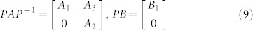 |
with  ,
,  , and
, and  , 1 ≤ n1 ≤ n and n1 + n2 = n. Otherwise (A, B) is said to be irreducible.
The dimension of the controllable subspace of structural system (A, B) varies as a function of free parameters in structural matrices A and B. That is, for different admissible systems ( ), the dimensions of their controllable subspaces might be different. As the maximum rank of matrix C is at most n, the dimension of controllable subspace of structural system (A, B) can reach the maximum value. We define this maximum value as the generic dimension of the controllable subspace of structure system (A, B) and denote it by GDCS(A,B). The GDCS(A,B) is a generic property31,32,38 in the sense that for almost all admissible systems
  (with respect to (A, B)) the dimension of their controllable subspaces takes a constant which is GDCS(A,B). Hosoe has proved38 that if (A, B) is irreducible. Then
 |
where G* denotes the set of subgraphs of G(A, B), which is defined as
 |
 denotes the number of edges in G. Applying equations (7) to the structural system (A,B), identifying the steering kernel by which the network G(A) can be transited between a state x0 and the origin becomes finding a structural control matrix B with the minimum number of columns such that
 |
Our second key result is that we develop a graph-theoretic algorithm39 to identify the steering kernel by solving an optimal assignment problem of a weighted bipartite graph (Figure 1e). For details, see the Materials and Methods and the Supplementary Information III.
Transittability of complex networks
We apply our algorithm to 27 complex networks to determine their steering kernels and the results are summarized in Table 1. These 27 networks are a portion of 38 complex networks in ref. 7,8 and the number of their nodes ranges from 32 to 27772 while the number of edges ranges from 96 to 352807. The phenotypes of complex networks are typically defined by a small portion of nodes40,41. For examples, the number of molecules (such as genes or proteins) significantly involved in a specific human disease is only a small portion of all molecules in a network4,5,11,12. Therefore, this study assumes that a transition between two specific states has 20% or 50% of nodes whose state values are changed, that is, x0 in (7) and (8) has 20% or 50% of nonzero elements. The fraction of steering nodes is defined as the ratio of the size of steering kernel to the total number of nodes in the networks. Columns 5–8 in Table 1 are the average results of 1000 randomly defined transitions of each network. Columns 7 and 8 respectively list the average fraction of steering nodes for transittability of 20% and 50% of nodes which are differently expressed at two states while Column 9 lists the fraction of driver nodes from Liu et al7. Comparing Columns 7 and 8 to Column 9 concludes that the minimum numbers of steering nodes required for transittability is much less than those for complete controllability. For complete controllability, the generic dimension of controllable space is the number of nodes in the networks listed in Column 3. Columns 5 and 6 respectively list the average generic dimension of controllable space for transittability of 20% and 50% of nodes which are differently expressed at two states. Comparing Columns 5 and 6 to Column 3 concludes that the controllable spaces for transittability are much smaller than those for complete controllability.
Table 1. Comparison of transittability and complete controllability of complex networks.
| Types | Network | Nodes | Edges | GDCS20% | GDCS50% |  |
 |
 |
|---|---|---|---|---|---|---|---|---|
| Regulatory | TRN-yeast-1 | 4441 | 12873 | 1014.05 | 2359.94 | 0.200 | 0.499 | 0.965 |
| TRN-yeast-2 | 688 | 1079 | 171.25 | 396.513 | 0.191 | 0.465 | 0.821 | |
| TRN-EC-1 | 1858 | 4123 | 407.11 | 1008.55 | 0.199 | 0.494 | 0.891 | |
| TRN-EC-2 | 418 | 519 | 105.32 | 236.61 | 0.185 | 0.434 | 0.751 | |
| OwnershipUSCorp | 7253 | 6726 | 1619.58 | 3758.57 | 0.190 | 0.460 | 0.820 | |
| Trust | CollegeStu | 32 | 96 | 29.44 | 31.911 | 0.133 | 0.186 | 0.188 |
| PrisonIn | 67 | 182 | 50.66 | 56.769 | 0.055 | 0.087 | 0.134 | |
| Wiki-Vote | 7115 | 103689 | 3013.03 | 4401.63 | 0.144 | 0.290 | 0.666 | |
| Food web | GrassLand | 88 | 137 | 31.94 | 65.68 | 0.147 | 0.346 | 0.523 |
| LittleRock | 183 | 2484 | 80.55 | 129.72 | 0.138 | 0.313 | 0.541 | |
| SeaGrass | 49 | 226 | 28.1 | 43.17 | 0.161 | 0.257 | 0.265 | |
| Ythan | 135 | 601 | 60.05 | 106.51 | 0.189 | 0.381 | 0.511 | |
| Metabolic | C.elegans | 1173 | 2864 | 896.86 | 1057.42 | 0.114 | 0.233 | 0.302 |
| E.coli | 2275 | 5763 | 1579.91 | 1955.38 | 0.129 | 0.276 | 0.382 | |
| S.cerevisiae | 1511 | 3833 | 1134.62 | 1352.12 | 0.119 | 0.248 | 0.329 | |
| Electronic circuit | S208 | 122 | 189 | 75.033 | 103.05 | 0.085 | 0.157 | 0.238 |
| S420 | 252 | 399 | 161.01 | 213.89 | 0.080 | 0.151 | 0.234 | |
| S838 | 512 | 819 | 325.05 | 433.43 | 0.076 | 0.147 | 0.232 | |
| Citation | HepTh | 27772 | 352807 | 19374.67 | 23329.95 | 0.085 | 0.134 | 0.216 |
| Internet | p2p-1 | 10876 | 39994 | 6534.15 | 9501.12 | 0.180 | 0.433 | 0.552 |
| p2p-2 | 8846 | 31839 | 5032.99 | 7572.36 | 0.183 | 0.446 | 0.578 | |
| p2p-3 | 8717 | 31525 | 5011.69 | 7515.04 | 0.185 | 0.451 | 0.577 | |
| Intra-organization | Consulting | 46 | 879 | 46 | 46 | 0.043 | 0.043 | 0.043 |
| Freemans1 | 34 | 6995 | 34 | 34 | 0.029 | 0.029 | 0.029 | |
| Freemans2 | 34 | 830 | 34 | 34 | 0.029 | 0.029 | 0.029 | |
| Manufacturing | 77 | 2228 | 77 | 77 | 0.013 | 0.013 | 0.013 | |
| Social | UCIOnline | 1899 | 20296 | 1338.29 | 1516.42 | 0.043 | 0.133 | 0.323 |
Notations are as follows: The average generic dimension of controllable space (GDCS20% and GDCS50%) for 20% and 50% of nodes changed between two specific states, respectively; the average fractions of steering nodes ( and
and  ) from our methods for 20% and 50% of nodes changed between two specific states, respectively; and fraction of driver nodes (
 ) from Liu's paper7
Applications to regulatory biomolecular networks
We employ four different biological systems with different phenotypes in order to demonstrate the applicability of our method, as well as validate our theoretical results. These four examples are p53-mediated DNA damage response network18 (three phenotypes), T helper differentiation cellular network19 (three phenotypes), yeast cell cycle network42 (three phenotypes), and epithelial to mesenchymal transition network (two phenotypes)20. Table 2 shows the identified steering kernels for transition between two phenotypes.
Table 2. The number of molecules, interactions and steering nodes.
| Network | Nodes | Edges | Phenotype Transitions | # of steering Nodes |
|---|---|---|---|---|
| p53- mediated DNA damage response network | 17 | 39 + 1(self-loop) | normal-arrest | 2(Wip1, p53DINP1) |
| normal-apoptosis | 2 (PTEN, p53DINP1) | |||
| arrest-apoptosis | 3(Wip1, PTEN, p53DINP1) | |||
| T helper differentiation cellular network | 17 | 25 + 2(self-loops) | Th0-Th1 | 2(SOCS1,T-bet) |
| Th0-Th2 | 2 (IL-4, GATA3) | |||
| Th1-Th2 | 2(T-bet, GATA3) | |||
| Yeast cell cycle network | 11 | 29 + 5(self-loops) | Phenotype 1–2 | 1 (SBF) |
| Phenotype 1–3 | 1(MBF) | |||
| Phenotype 2–3 | 1(SBF) | |||
| EMT network | 6 | 15 | epithelial - mesenchymal | 1 (any node except for CDH1) |
p53-mediated DNA damage response network
This network, consisting of 17 molecules and 40 interactions as shown in Figure 2 and Table S1, responds to cell stresses such as DNA damage and can stay at three phenotypes18. If there is no DNA damage, the ATM is inactive (ATM2). The level of phosphorylated monomer (ATM*) is low, then the p53 remains inactive. The DNA damage can lead to two different cellular phenotypes: cell cycle arrest and apoptosis18. At the cell cycle arrest phenotype, ATM is activated by DNA damage through auto-phosphorylation and transited from inactive dimer (ATM2) to ATM*. Subsequently, p53 is activated by ATM* and transited to p53*(p53 arrester). The expression levels of molecules represented by those green nodes in Figure 2 are oscillating18. The p21 is the product of this state which induces cell arrest. In total, the expression values of 9 nodes are significantly changed when the normal phenotype is transited to the arrest phenotype. At the apoptosis phenotype, ATM* still activates p53 to p53*, but most p53* are in form of p53 killer. P53AIP1 is activated by p53 killer and finally activates Casp3 which induces cell apoptosis. At this state, PTEN contributes to full activation of p53. In total, the expression values of 12 nodes are significantly changed when the normal phenotype is transited to the apoptosis phenotype. In addition, comparing the arrest phenotype and the apoptosis phenotype, the expression values of all 17 nodes are significantly changed. Applying our methods to this network yields the steering kernel consisting of PTEN and p53DINP1 for the transition between normal and apoptosis phenotypes; the steering kernel consisting of Wip1 and p53DINP1 for the transition between normal and cell cycle arrest phenotypes; and the steering kernel consisting of Wip1, PTEN and p53DINP1 for the transition between apoptosis and cell cycle arrest phenotypes. These results are in great agreement with Zhang et al's results18 where PTEN and Wip1 are identified as key players for transitions of different states. On the other hand, if the complete controllability7 is applied to this network (Figure S5), the minimum number of driver nodes is 3 while the driver nodes are not unique. For example, one minimum set of driver nodes consists of Wip1, PTEN and p53DINP1, which are the same as the steering nodes for transition between apoptosis and cell cycle arrest phenotypes. However, this set of nodes for other two transitions is redundant. Furthermore, the complete control strategy with these three driver nodes will affect the full state space during the phenotype transition as shown in Table 2, which is clearly undesirable in practice (see Discussion).
Figure 2. P53-mediated cell damage response network and its phenotype transitions.

A green-filled node means the level of this node oscillating at that state, a red-filled node means high level while an empty node means low level. The steering kernels are labelled for different transitions.
T helper differentiation cellular network
T helper cells (Th cells) are a sub-group of lymphocytes, a type of white blood cells, which play an important role in the immune system, particularly in the adaptive immune system. They help the activity of other immune cells by releasing T cell cytokines43,44,45. Matured Th cells express the surface protein CD4 and are referred to as CD4+T cells which can be classified as Th0 (precursor), Th1 and Th2 (effector) cells. Previously published experiments43,44 suggest that T-bet and GATA3 can induce both transitions from Th0 to TH1 and from Th0 to Th2. To deeply understand the mechanism of transitions among these phenotypes, Mendoza19 constructs a core network in charge of the differentiation of Th cells, which contains 17 nodes with 27 interactions as shown in Figure 3 and Table S2. Comparing among these three phenotypes, one can see that 5, 4, and 9 molecules are significantly differentially expressed, between Th0 and Th1 phenotypes, between Th0 and Th2 phenotypes, and between Th1 and Th2 phenotypes, respectively. Applying our methods to the T helper differential cellular network19, we identify the steering nodes SOCS1 and T-bet for the transition between Th0 and Th1 and the steering nodes IL-4 and GATA3 for the transition between Th0 and Th2, which is in agreement with existing results43,44. We also identify the steering nodes T-bet and GATA3 for the transition between Th1 and Th2, which is completely in agreement with the experimental data43,45. However, if the complete controllability7 is applied to this network (see Figure S6), the minimum number of driver nodes is three and the three driver nodes are IL-12, IL-18 and IFN-β. Actually, without any one of these three nodes, this network cannot be completely controlled. Although it has been reported that IL-12 and IL-18 together can make the transition from Th0 to Th1, this complete control strategy will affect the full state space during the transition as shown in Table 2, which is undesirable in practice (see Discussion).
Figure 3. T helper differentiation cellular network and its phenotype transitions.

A red-filled node means high level expression and an empty node means low level expression. The steering kernels are labelled for different transitions.
Yeast cell cycle network
The cell-cycle process is a vital biological process by which one cell grows to divide into two daughter cells. To study this process, Li, et al42 have established a molecular network consisting of 11essential molecules with 34 interactions as shown in Figure 4 and Table S3. Applying the logic-like operations and using the exhaustive search, they have found seven stationary states (attractors), each corresponding a stable phenotype. The attractor with the largest basin size corresponds to the G1 stationary state of the cell (denoted by phenotype 1). The next two largest attractors may represent some common disorder states of the cell (denoted by phenotypes 2 and 3). As other four attractors have small basin sizes, we do not consider them in this study. Comparing among these three phenotypes, we can see that 4, 1, and 5 nodes are significantly differentially expressed, between phenotypes 1 and 2, between phenotypes 1 and 3, and between phenotypes 2 and 3, respectively. On the one hand, the result by applying complete controllability7 to this network is that the minimum number of driver nodes is 1 which could be Cln3, MBF or SBF (Figure S7). However, via either MBF or SBF this network cannot be completely controlled as either of them does not regulate node Cln3 from Figure 4. Although via Cln3 the network can be completely controlled, the full state space will be affected as shown in Table 2, which is undesirable (see Discussion). On the other hand, we apply our methods to this network for studying the transitions among those three phenotypes. We found a single steering node MBF for the transition between phenotypes 1 and 3, and a single steering node SBF for both the transition between phenotypes 1 and 2 and the transition between phenotypes 2 and 3, which suggests that SFB and MBF play an important role for the transitions among these three phenotypes in the cell-cycle process.
Figure 4. Yeast cellular network and its phenotype transitions.

A red-filled node means high level expression while an empty node means low level expression. The steering kernels are labelled for different transitions.
Epithelial to Mesenchymal Transition (EMT) network
EMT is a phenomenon that cells change their genetic and transcriptional program leading to the alteration of phenotypes and functions. This change starts the metastatic dissemination which causes most human cancer deaths20. To study EMT, Moes et al20 have constructed an EMT network consisting of 6 nodes and 15 interactions as shown in Figure 5 and Table S4. The expressions of MIR203, MIR200 and CDH1 are high and ZEB2, SNAI1 and ZEB1 are low at the epithelial phenotype while all are reversed at mesenchymal phenotype. Therefore, for this network, all 6 nodes are significantly differentially expressed between epithelial and mesenchymal phenotypes. Applying our algorithm, we can identify node SNAI1 as the steering node for the transition of these two phenotypes, which is completely in agreement with the experimental result verified by Moes et al20 that SNAI1 can activate the transition from epithelial to mesenchymal phenotype. Actually, by applying our algorithm, we can identify anyone of all nodes except for CDH1 as the steering node for the transition of these two phenotypes. From the other recent literature20,46, MIR203 and MIR200 can also induce the transitions while leaving ZEB2 and ZEB1 deserving the further investigation about their function for the transition between these two phenotypes. In fact, controlling the transition between these two phenotypes is complete control of the network. When the minimum input theorem7 is applied to this network (Figure S8), anyone of six nodes could be the driver node to steer the network from one phenotype to any other phenotype. However, acting input control signals on CDH1 cannot make the transition between these two phenotypes as CDH1 does not regulate any nodes in the network from Figure 5.
Figure 5. EMT network and its phenotype transitions.
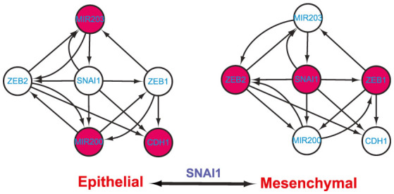
A red-filled node means high level expression while an empty node means low level expression. One of steering kernels is labelled for the transition.
Discussion
Transittability is at the heart of understanding state transitions of complex dynamic systems, especially cellular processes such as the cellular reprogramming and genetic disorder progressions. Besides the empirical studies20,21,22,23,24,25,26, recently control theory for dynamical systems28,29 has been applied to complex systems. As indicated in discussions33,35,47 and Supplementary Information I, complete controllability of complex networks7 generally needs more steering nodes and its control affects the full state space (Figure 1b), and thus are not suitable to study the transittability and to identify the steering kernel for state transitions. Although the recently developed control strategy of nonlinear systems10 is applicable to study the transittability, it needs to know the exact expression of nonlinear functions and parameters in the model of complex systems, which is generally unavailable in practice7.
Instead of steering a directed network from any initial state to any desired state with the concept of complete controllability, transittability concerns the ability to steer a directed network from one specific state to another specific state. Obviously if a directed network is completely controllable, it can be steered from one specific state to another specific state, which indicates that complete controllability is sufficient for transittability. However, complete controllability is not necessary for transittability and should even be avoided in practice. For example, when considering the transition from a disease phenotype to a healthy phenotype, we expect to affect as a small state subspace as possible because side effects might be caused by unnecessarily changing some nodes in a large state subspace. The state subspace affected by a control law can be measured by the generic dimension of controllable (sub) space. The GDCS for complete controllability is always the full dimensional state space while the GDCS for two state transittability is generally a small subspace of the full state space (see Tables 1 and 3). Therefore, in principle the control law based on the complete controllability affects states more than the one based on the transittability. In addition, as discussed in Supplementary Information I, a network cannot be guaranteed to transit from one specific state to any other state by acting the input control signals on only the minimum set of driver nodes identified by the minimum input theorem7. Furthermore, although theoretically the steering kernel could be a subset of the minimum driver nodes7, the minimum input theorem7 cannot be applied for efficiently finding the minimum number of steering nodes. Firstly, although the minimum number of driver nodes identified by minimum input theorem7 is unique, the maximum matching for a given network is not unique. Actually finding all maximum matchings for a given network is an NP-hard problem. This means that there is no efficient way to find all possible sets of driver nodes. Secondly, by the minimum input theorem7, the minimum number of driver nodes is about 0.8 n for regulatory networks with n nodes. All possible combinations of 0.8 n driver nodes is at least 20.8n, and thus it is computationally prohibitive to exhaustively check all of them.
Table 3. GDCS for complete controllability and transittability.
| Network | GDCS for complete controllability | Phenotype Transitions | GDCS for transittability |
|---|---|---|---|
| p53- mediated DNA damage response network | 17 | normal-arrest | 16 |
| normal-apoptosis | 16 | ||
| arrest-apoptosis | 17 | ||
| T helper differentiation cellular network | 17 | Th0–Th1 | 12 |
| Th0–Th2 | 12 | ||
| Th1–Th2 | 12 | ||
| Yeast cell cycle network | 11 | Phenotype 1–2 | 10 |
| Phenotype 1–3 | 10 | ||
| Phenotype 2–3 | 10 | ||
| EMT network | 6 | epithelial - mesenchymal | 6 |
In this paper, we have systematically studied the transittability of directed networks and proposed an algorithm to identify the steering kernel for transitions between two specific states. To bypass the needs of knowing the exact expression of nonlinear functions and parameters in the complex systems, we have studied the transittability of directed networks with the concepts of structural linear systems and structural transittability. Our theoretical results provide the sufficient and necessary condition for determining the transittability, which is to check whether or not two GDCSs are equal. Although our theorems have been developed with continuous time-invariant linear systems, they can be directly applied to discrete time-invariant linear systems. Therefore, similar to the theorems48, our results remain unchanged even if the free parameters in a linear system are allowed to vary with time. That is, our theoretical results are applicable to time-varying linear systems.
To identify the steering nodes for the transition between two states, we have developed a graph-theoretic algorithm by solving an optimal assignment problem of a weighted bipartite graph39. Applying our algorithms to 27 complex networks we have found that the minimum numbers of steering nodes for transiting two states are less than those for complete controllability and the controllable spaces for transittability are smaller than those for complete controllability. Furthermore we have applied our algorithm to 4 regulatory biomolecular networks and found that the numbers of steering nodes for transiting two cellular phenotypes are small, which is greatly in agreement with empirical studies on these networks. In addition, majority of steering nodes found by our method have been already reported in existing empirical studies while other new steering nodes are potentially important in corresponding cellular phenotype transitions. Therefore, we believe that our results also provide some fundamentals for understanding the mechanism of cellular phenotype transitions, and as such, are expected to have implications for network-based drug design. As can be seen, the theorems we developed in this study can directly be applied to any other complex networks, for example, social networks, power grids, food webs, the Internet, and electronic circuits7,8, just named a few. In this paper, we mainly focused on studying transittability with suitable input signals, and the implementation or design of the control input signals as well as analysis of the dependence between the size of steering kernel and the degree distribution of networks could be one direction of future work.
Methods
Network construction
The T helper differentiation cellular network, the EMT network, and the yeast cell cycle network are directly from the published references19,20,42 without any change, respectively. The P53 mediated DNA damage response network are constructed from the differential equations in the supplementary material of the paper18. In such a construction, each variable in the differential equations corresponds to a node in the network. Node i regulates node j if the variable corresponding to node i appears in the right-handed side of the differential equation corresponding to node j. All self-loops corresponding to the degradations are excluded in the constructed network as their weights may not be free parameters.
Calculating the GDCS and the size of the steering kernel
For a network G(A) and structural state x0, assume that the structure system (A, x0) is irreducible. Let S be a subset of nodes corresponding to non-zero components in x0. Let us define a weighted graph G′(A) as follows: 1) associate the weight we = 1 with every edge e of G(A); 2) add the edge e = vivj and associate the weight we = ε if e = vivj is not in G(A) for  ; 3) add the loop e = vivi and associate the weight we = 0 if e = vivi is not in G(A) for
  , where ε is a small positive number and less than 1/n for a network with n nodes. For simplicity, ε can take the value of 0.001, 0.0001, 0.00001 or the like. By solving an optimal assignment of a weighted bipartite graph representation of G′(A), we can find the maximum weight circle partition of G′(A). Assume that the weight of the maximum circle partition is r + s*ε, where r and s are integers and s*ε < 1. Let t be the number of source strong connected components of G(A). Then, from Supplementary Information III.C, we have GDCS(A, B) = GDCS(A, B0) = r + s and the size of steering kernel is s + t. Note that the computational complexity of solving an optimal assignment of a weighted bipartite graph is O(n3) according to reference39 for the worst cases in which a network is a complete graph. For the sparse networks which are true in most cases, our computational complexity is less than O(n3). Actually Table S5 and Figure S9 show that the our computational complexity is approximately O(n2.35) for real complex networks with the number of nodes from 32 to 27772.
Author Contributions
F.X.W., L.C. and J.L. conceived the study; F.X.W. developed the theoretical results and was the lead writer of the manuscript; F.X.W. and L.W. and J.W. developed the algorithms and designed the numerical simulation and performed the actual experimental data analysis; all the authors modified the manuscript and approved the final version.
Supplementary Material
SI201404FFWithFigures
Acknowledgments
This work was supported by Natural Sciences and Engineering Research Council of Canada (NSERC) through FXW, by the National Natural Science Foundation of China under Grant No. 61232001 through JXW, by National Natural Science Foundation of China (61272274) and Program for New Century Excellent Talents in Universities (NCET-10-0644) through JL, and by the National Natural Science Foundation of China (Grant Nos. 61134013, 91029301, and 11326035) and the FIRST program from JSPS initiated by CSTP through LC.
References
- Newman M., Barabási A. L. & Watts D. J. The Structure and Dynamics of Networks (Princeton University Press, New Jersey, 2006).
- Barabási A. L., Gulbahce N. & Loscalzo J. Network medicine: a network-based approach to human disease. Nat. Rev. 12, 56–68 (2011). [DOI] [PMC free article] [PubMed] [Google Scholar]
- Barabási A. L. & Oltvai Z. N. Network biology: Understanding the cell's functional organization. Nat. Rev. Genet. 5, 101–113 (2004). [DOI] [PubMed] [Google Scholar]
- Vidal M., Cusick M. E. & Barabási A. L. Interactome networks and human disease. Cell 144, 986–998 (2011). [DOI] [PMC free article] [PubMed] [Google Scholar]
- Goh K. I. et al. The human disease network. Proc. Natl. Acad. Sci. 104, 8685–8690 (2007). [DOI] [PMC free article] [PubMed] [Google Scholar]
- Yildirim M. A., Goh K. I., Cusick M. E., Barabási A. L. & Vidal M. Drug-target network. Nat. Biotechnol. 25, 1119–1126 (2007). [DOI] [PubMed] [Google Scholar]
- Liu Y. Y., Slotine J. J. & Barabási A. L. Controllability of complex networks. Nature 473,167–173 (2011). [DOI] [PubMed] [Google Scholar]
- Nepusz T. & Vicsek T. Controlling edge dynamics in complex networks. Nat. Phys. 8, 568–573 (2012). [Google Scholar]
- Nacher J. C. & Akutsu T. Structural controllability of unidirectional bipartite networks. Sci. Rep. 3, 1647; 10.1038/srep01647 (2013). [DOI] [PMC free article] [PubMed] [Google Scholar]
- Cornelius S. P., Kath W. L. & Motter A. E. Realistic control of network dynamics. Nat. Commun. 4, 1942; 10.1038/ncommx2939 (2013). [DOI] [PMC free article] [PubMed] [Google Scholar]
- Chen L., Liu R., Liu Z. P., Li M. & Aihara K. Detecting early-warning signals for sudden deterioration of complex diseases by dynamical network biomarkers. Sci. Rep. 2, 342; 10.1038/srep00342 (2012). [DOI] [PMC free article] [PubMed] [Google Scholar]
- Liu R. et al. Identifying critical transitions and their leading biomolecular networks in complex diseases. Sci. Rep. 2, 813; 10.1038/srep00813 (2012). [DOI] [PMC free article] [PubMed] [Google Scholar]
- Hartwell L. H., Hopfield J. J., Leibler S. & Murray A. W. From molecular to modular cell biology. Nature 402, C47–C52 (1999). [DOI] [PubMed] [Google Scholar]
- Kitano H. Computational systems biology. Nature 420, 206–210 (2002). [DOI] [PubMed] [Google Scholar]
- Yang K., Bai H., Ouyang Q., Lai L. & Tang C. Finding multiple target optimal intervention in disease-related molecular network. Mol. Syst. Biol. 4, 228(2008). [DOI] [PMC free article] [PubMed] [Google Scholar]
- Milo R. et al. Network motifs: Simple building blocks of complex networks. Science 298, 824–827 (2002). [DOI] [PubMed] [Google Scholar]
- Butcher E. C., Berg E. L. & Kunkel E. J. Systems biology in drug discovery. Nat. Biotechnol. 22, 1253–1259 (2004). [DOI] [PubMed] [Google Scholar]
- Zhang X. P., Liu F. & Wang W. Two-phase dynamics of p53 in the DNA damage response. Proc. Natl. Acad. Sci. USA. 108, 8990–8995 (2011). [DOI] [PMC free article] [PubMed] [Google Scholar]
- Mendoza L. A network model for the control of the differentiation process in Th cells. BioSystems 84, 101–114 (2006). [DOI] [PubMed] [Google Scholar]
- Moes M. et al. A novel network integrating a miRNA-203/SNAI1 feedback loop which regulates epithelial to mesenchymal transition. PLoS ONE 7, e0035440; 10.1371/journal.pone. 0035440 (2012). [DOI] [PMC free article] [PubMed] [Google Scholar]
- Takahashi K. & Yamanaka S. Induction of pluripotent stem cells from mouse embryonic and adult fibroblast cultures by defined factors. Cell 126, 663–676 (2006). [DOI] [PubMed] [Google Scholar]
- Kim J. B. et al. Oct4-induced pluripotency in adult neural stem cells. Cell 136,411–419 (2009). [DOI] [PubMed] [Google Scholar]
- Vierbuchen T. et al. Direct conversion of fibroblasts to functional neurons by defined factors. Nature 463, 1035–1041 (2010). [DOI] [PMC free article] [PubMed] [Google Scholar]
- Ieda M. et al. Direct reprogramming of fibroblasts into functional cardiomyocytes by defined factors. Cell 142, 375–386 (2010). [DOI] [PMC free article] [PubMed] [Google Scholar]
- Szabo E. et al. Direct conversion of human fibroblasts to multilineage blood progenitors. Nature 468, 521–526 (2010). [DOI] [PubMed] [Google Scholar]
- Huang P. et al. Induction of functional hepatocyte-like cells from mouse fibroblasts by defined factors. Nature 475, 386–389 (2011). [DOI] [PubMed] [Google Scholar]
- Schenk T. et al. Inhibitions of the LSD1 (KDM1A) demethylase reactivates the all-trans-retinoic acid differentiation pathway in acute myeloid leukemia. Nat. Med. 18, 605–611 (2012). [DOI] [PMC free article] [PubMed] [Google Scholar]
- Rosenbrock H. H. State-Space and Multivariable Theory (Thomas Nelson and Sons LTD, London, 1970).
- Lombardi A. & Hörnquist M. Controllability analysis of networks. Phys. Rev. E 75, e056110; 10.1103/PhysRevE.75.056110 (2007). [DOI] [PubMed] [Google Scholar]
- Lin C. T. Structural controllability. IEEE Trans Auto Contr. 19, 201–208 (1974). [Google Scholar]
- Shields R. W. & Pearson J. B. Structural controllability of multi-input linear systems. IEEE Trans Auto Contr. 21, 201–208 (1976). [Google Scholar]
- Commault C., Dion J.-M. & van der Woude J. W. Characterization of generic structural properties of linear structured systems for efficient computations. Kybernetika 38, 503–520. (2002) [Google Scholar]
- Müller F. J. & Schuppert A. Few inputs can reprogram biological networks. Nature 478, 10.1038/nature10543 (2011). [DOI] [PubMed] [Google Scholar]
- Huang S., Eichler G., Bar-Yam Y. & Ingber D. E. Cell fates as high-dimensional attractor states of a complex gene regulatory network. Phys. Rev. Lett. 94, e128701; 10.1103/PhysRevLett. 94. 128701 (2005). [DOI] [PubMed] [Google Scholar]
- Liu Y. Y., Slotine J. J. & Barabási A. L. Few inputs can reprogram biological networks (reply by Liu et al.). Nature 478, 10.1038/nature10544 (2011). [Google Scholar]
- Slotine J.-J. & Li W. Applied Nonlinear Control (Prentice-Hall, ew Jersey, 1991).
- Yuan Z. Xiao C., Wang X. X. & Lai Y. C. Exact controllability of complex networks. Nature Communications 4, 2447 10.1038/ncomms 3447 (2013). [DOI] [PMC free article] [PubMed] [Google Scholar]
- Hosoe S. Determination of generic dimensions of controllable subspaces and its application. IEEE Trans Auto Contr. 25, 1192–1196 (1980). [Google Scholar]
- Jungnickel D. Graphs, Networks and Algorithms (Springer, New York, 2005).
- Choi M., Shi J., Jung S. H., Chen X. & Cho K.-H. Attractor landscape analysis reveals feedback loops in the p53 network that control the cellular response to DNA damage. Sci. Signal. 5, ra83 (2012). [DOI] [PubMed] [Google Scholar]
- Kim J., Park S. & Cho K. Discovery of a kernel for controlling biomolecular regulatory networks. Sci. Rep. 3, 2223; 10.1038/srep02223 (2013). [DOI] [PMC free article] [PubMed] [Google Scholar]
- Li F., Long T., Lu Y., Ouyang Q. & Tang C. The yeast cell-cycle network is robustly designed. Proc. Natl. Acad. Sci. USA. 101, 4781–4786 (2004). [DOI] [PMC free article] [PubMed] [Google Scholar]
- Lee H. J. et al. GATA-3 induces T helper cell type 2 (Th2) cytokine expression and chromatin remodeling in committed Th1 cells. J. Exp. Med. 192, 105–115 (2000). [DOI] [PMC free article] [PubMed] [Google Scholar]
- Szabo S. J., Kim S. T., Costa G. L., Zhang X., Fathman C. G. & Glimcher L. H. A novel transcription factor, T-bet, directs Th1 lineage commitment. Cell 100, 655–669 (2000). [DOI] [PubMed] [Google Scholar]
- Hwang E. S., Szabo S. J., Schwartzberg P. L. & Glimcher L. H. T helper cell fate specified by kinase-mediated interaction of T-bet with GATA-3. Science 307, 430–433 (2005). [DOI] [PubMed] [Google Scholar]
- Park S. M., Gaur A. B., Lengyel E. & Peter M. E. The miR-200 family determines the epithelial phenotype of cancer cells by targeting the E-cadherin repressors. Genes Dev. 22, 894–907 (2008). [DOI] [PMC free article] [PubMed] [Google Scholar]
- Cowan N. J. Chastain E. J., Vilhena D. A., Freudenberg J. S. & Bergstrom C. T. Nodal dynamics, not degree distributions, determine the structural controllability of complex networks. PLoS ONE 7(6), e38398; 10.1371/journal.pone.0038398 (2012). [DOI] [PMC free article] [PubMed] [Google Scholar]
- Poljak S. On the generic dimension of controllable subspaces. IEEE Trans Auto Contr. 35, 367–369 (1990). [Google Scholar]
Associated Data
This section collects any data citations, data availability statements, or supplementary materials included in this article.
Supplementary Materials
SI201404FFWithFigures