A Parametrically Constrained Optimization Method for Fitting Sedimentation Velocity Experiments

Abstract

A method for fitting sedimentation velocity experiments using whole boundary Lamm equation solutions is presented. The method, termed parametrically constrained spectrum analysis (PCSA), provides an optimized approach for simultaneously modeling heterogeneity in size and anisotropy of macromolecular mixtures. The solutions produced by PCSA are particularly useful for modeling polymerizing systems, where a single-valued relationship exists between the molar mass of the growing polymer chain and its corresponding anisotropy. The PCSA uses functional constraints to identify this relationship, and unlike other multidimensional grid methods, assures that only a single molar mass can be associated with a given anisotropy measurement. A description of the PCSA algorithm is presented, as well as several experimental and simulated examples that illustrate its utility and capabilities. The performance advantages of the PCSA method in comparison to other methods are documented. The method has been added to the UltraScan-III software suite, which is available for free download from http://www.ultrascan.uthscsa.edu.

Introduction

Analytical ultracentrifugation is an important method for studying macromolecular systems in the solution phase. This technique can be used to obtain detailed information about dynamic interactions of macromolecules and to describe the composition of mixtures, including partial concentration of its constituents as well as their molar mass and anisotropy distributions. In recent years, in part due to the availability of fast and low-cost computers, significant advances have been made in the sophistication of data analysis methods and software for the study of sedimentation velocity (SV) experiments. SV experiments can be modeled by finite-element solutions of the Lamm equation (1), but such solutions are computationally considerably more complex than exponential functions used for sedimentation equilibrium experiments. However, the computational complexity incurred when analyzing SV experiments is offset by the significant advantage in information that SV experiments offer, especially with respect to resolution and precision (2).

Unlike in equilibrium experiments, where net flow ceases in the ultracentrifuge cell, the sedimentation and diffusion transport in SV experiments incurs frictional effects arising from the interaction of the macromolecules with the surrounding solvent. These frictional effects can be measured, and as long as the partial specific volumes (PSV) of the solutes are known, they can be conveniently expressed in terms of the frictional ratio, f/f₀, or anisotropy. This quantity relates the frictional coefficient f of each solute to the frictional coefficient of a hypothetical sphere that has the same density and volume as the solute. If the molecule is spherical, these coefficients are identical, and the frictional ratio equals unity. For molecules with increasing nonglobularity, the frictional ratio increases to values of 1.2–1.5 for folded proteins, up to 2.5 for intrinsically disordered and denatured proteins, and to much larger values for fibrils, elongated polymer chains, and linear nucleic acids.

In addition, the sedimentation and diffusion coefficients, together with the PSV, can be used to infer the molar mass distributions of the solutes. A complete description of the molar mass and anisotropy of each distinct solute in the mixture is therefore possible, provided the solutes are observed with a sufficient signal/noise. It should be noted that we refer to the PSV and frictional ratio of the sedimenting particle observed in the analytical ultracentrifuge, which includes hydration. Previously, we described the two-dimensional spectrum analysis (2DSA) (3,4), which solves the problem of modeling the sedimentation coefficient and anisotropy distributions of heterogeneous mixtures for the general case by decomposing the domain of possible solutes into a high resolution two-dimensional grid of sedimentation and diffusion coefficient pairs. In this fitting method, a Lamm equation (1) solution is simulated for each sedimentation and diffusion coefficient pair, and a linear combination of all simulated solutions is fitted by a nonnegatively constrained least-squares (NNLS) algorithm (5) to the experimental data. In this linear fit, the solution is represented by positive, nonzero coefficients of each term in the linear combination.

In the 2DSA, the high-resolution grid used includes many more solutes than can be resolved by the technique, and therefore the solution is subject to considerable degeneracy, and especially for noisy data, produces false positives, albeit with low concentrations. This problem can be addressed by performing a parsimonious regularization on the result using genetic algorithms (6). However, the refinement of the 2DSA solution by genetic algorithms using a parsimonious regularization approach is only appropriate for paucidisperse solute systems. For systems where broad heterogeneity is evident, the resolution afforded by sedimentation velocity experiments is insufficient to identify individual solutes in the mixture by genetic algorithms, and a 2DSA Monte Carlo approach is more appropriate. Monte Carlo analysis will attenuate noise contributions, and regularize the final solution (7). Although this method can provide high-resolution detail, we will show that for certain polymerizing systems, additional constraints imposed on the grid will reduce the degeneracy without decreasing the quality of the fit, and avoid any ambiguity that may result from the overdetermined grid, and thus improve the information content.

Theory and Algorithm

A constrained grid method for the characterization of macromolecular mixtures that are heterogeneous both in size and anisotropy was implemented in the software UltraScan-III (The University of Texas Health Science Center at San Antonio (UTHSCA), San Antonio, TX). The method, termed parametrically constrained spectrum analysis (PCSA), discretizes the sedimentation and diffusion coefficients along an arbitrary function f/f₀ = F(s) over a space S defined by user-specified limits s_min, s_max, f/f_0,min, and f/f_0,max. There is no limitation on the functional form of F, as long as it is single-valued, which constitutes the constraint. The functional form of F should also describe the distribution characteristics of the solutes in the system to be fitted. Multiple functional forms can be tested to identify the most appropriate function. Analogous to the 2DSA method, each discretized point along the curve described by F(s) gives rise to a parameter pair consisting of a sedimentation coefficient and a frictional ratio. A corresponding diffusion coefficient D is obtained from the expression shown as

$$D=RT{\left[Nk9\eta \pi \sqrt{\frac{2sk\overline{\nu }\eta }{1-\overline{\nu }\rho }}\right]}^{-1},$$ (1)

where R is the universal gas constant, T is the temperature of the experiment, N is Avogadro’s number, k is the frictional ratio f/f₀, η is the viscosity, ρ is the density of the solvent, and $\overline{\nu }$ denotes the PSV. The corresponding s and D values from each point in the discretization of F are used to simulate an entire experiment for each solute described by F, generating the inputs for a linear system shown as

$$Ax=b,$$ (2)

where A is the matrix containing all simulated data, x is the concentration vector to be solved by NNLS minimization, and b is the vector containing the experimental data. The simulations are generated with the adaptive space-time finite-element solution of the Lamm equation as described earlier in Cao and Demeler (8,9). After NNLS optimization, as represented in Eq. 3, a sparse linear combination of Lamm equations is obtained, and the final solution is described by Eq. 4,

$$\min {\Vert Ax-b\Vert }^2:x\ge 0,$$ (3)

$$C\left(r,t\right)=\sum _{i=1}^n{c}_{i}L\left(s_i,f/f_{0,i}\right)+h,$$ (4)

where C represents the concentration of the fitted solution for radius r and scan t, c_i is the fitted partial concentration (always a positive, nonzero value) for simulated component i, L is the Lamm equation solution for component i, and h represents a baseline offset incorporating time- and radially invariant noise components.

Because a single function F does not cover the entire space S that should be examined to capture all possible signals needed to represent the experimental system within the constraint of the functional form, a parameterization of the functional form is now required. For example, the functional form implemented in the C(s) method (10) uses a horizontal line within an f/f₀ versus s grid to represent all components in the experimental mixture. The parameterization of this functional form consists of varying the intercept of the horizontal line. Because the horizontal line in C(s) is constrained to a single f/f₀ value, heterogeneity in f/f₀ cannot be identified. However, a weight average frictional coefficient can still be obtained by evaluating multiple horizontal lines with different intercepts and finding the line giving rise to the lowest root mean-square deviation (RMSD). But even if a straight line is adopted as the functional form, the limitation of a single frictional ratio in the C(s) method can be overcome by not restricting the solutions to a horizontal line, but instead varying not only the intercept, but also the slope. In this article, we refer to the C(s) method by its horizontal-line parameterization as PCSA-HL.

To address the general case of variable frictional ratios, we have implemented an analogous approach by performing a grid search over a k-vector of parameters p = [p₁,p₂,…,p_k] of a functional form F(s,p) where the functional form itself can be varied. For each functional form F and vector of parameters p, we proceed as follows:

Each point of the discretization of F(s,p) over the user-specified search space S provides an s and D pair as input to the Lamm equation. This populates the columns of a matrix of simulated data A_F(s,p), which is subsequently fit to the experimental data b, providing an RMSD goodness-of-fit for each chosen F, p. The user then selects the discretization interval for p such that the variants of the functional form sufficiently cover the search space S. In these terms, the goal of the PCSA is to perform the optimization shown in

$$\min {\Vert A_{F\left(s,\mathbf{p}\right)}x-b\Vert }^2:F,\mathbf{p}\in \mathbf{p}\text{-grid},x\ge 0.$$ (5)

For example, when the functional form of F is represented by a straight line, then k = 2 and the parameters to be varied are the slope (p₁) and the intercept (p₂) of the straight line. In this case, the p-grid to be searched is constructed to ensure that the variations of p₁ and p₂ are chosen so that F(s,p) achieves a uniform coverage of the entire search space S. Other functional forms include, but are not limited to exponential growth or decay and increasing or decreasing sigmoids. An example of a low-resolution discretization with the functional form of a straight line (SL) is shown in Fig. 1 A, and for an increasing and decreasing sigmoid in Fig. 1, B and C, respectively. A higher resolution discretization is shown in Fig. 2 A. Each element of the p-grid defines an F(s,p) value, whose discretization produces a different linear combination of Lamm equations that populate the columns of matrix A.

Figure 1.

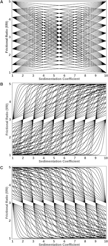
Low-resolution grid parameterizations using 10 grid variations for a two-dimensional grid covering the sedimentation coefficient range from 1 to 10 S and the anisotropy range for frictional ratios from 1 to 5 given by (A) straight-line models; (B) increasing sigmoid models; and (C) decreasing sigmoid models. Higher resolution is achieved by either iteratively increasing the resolution in a subsection of the grid, or by using denser grids.

Figure 2.

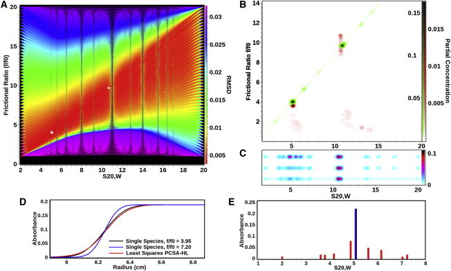
Comparison between different analysis methods applied to the experimental data listed in Table 2. (A) RMSD heat map for a high-resolution grid using the straight-line (SL) PCSA. (Red lines) Solutions with the lowest RMSD; (purple lines) poor selections for this system. (The BFM is the red line that intercepts the two white circles.) (White circles) Most prominent solutes found for this system in the BFM. (B) Genetic algorithm Monte Carlo analysis (red) overlaid with the straight-line PCSA Monte Carlo analysis (green). The major components are essentially congruent, exhibiting significant difference in anisotropy. The PCSA fit constrains the solution to a single point, while the genetic algorithm analysis is multivalued for the frictional ratio of the larger species. (C) PCSA horizontal-line parameterization (PCSA-HL) for the same data as analyzed in panel B. All fits have the same frictional ratio average of 7.20, but are shown offset for clarity: unregularized (top), TR with L-curve criterion α-value = 0.51 (center), 100-iteration Monte Carlo analysis (bottom). For all fits, the smaller species is significantly broadened in the s-domain through introduction of false positives as explained in panels D and E. One-dimensional histogram plots for the same data are shown for each plot in Fig. S1 in the Supporting Material. (D) Boundary shapes of two solutes with identical s-values of 5.07 s (equal to the smaller DNA species shown in panel B), but different f/f₀; (blue) f/f₀ = 7.20, the average value obtained in the PCSA-HL, and (black) f/f₀ = 3.95, which is equal to the true f/f₀ value of the smaller DNA species. (Red curve) Fit of the (black) curve obtained by PCSA-HL when f/f₀ is constrained to 7.20. (The red curve clearly has a much smaller deviation from the black curve than the blue curve, because the red curve satisfies the least-squares condition and produces a lower RMSD at the expense of introducing multiple artifactual solutes.) (E) Solutes obtained in the PCSA-HL fit of the (black) curve shown in panel D. (Black/blue position) The true single species position and partial concentration. All red bars, corresponding to the unregularized fit shown in the red curve in panel D, represent incorrect sedimentation coefficients, frictional ratios, and partial concentrations. This condition is encountered whenever a mixture heterogeneous in frictional ratio is fitted with the PCSA-HL or the C(s) method. As shown in panel B, this problem is completely eliminated by the PCSA-SL solution.

Each linear combination is solved according to Eq. 3, and all solutions are then ranked by RMSD. Because the calculation of any one solution is independent of another, these calculations can be performed in parallel. UltraScan-III takes advantage of multicore architectures to perform these calculations in multiple threads, allowing high-resolution grids to be calculated in a matter of seconds or minutes, depending on grid resolution and the number of cores available. A detailed performance analysis for a dataset with 20,000 datapoints is presented in Table S1 in the Supporting Material. After obtaining the optimal RMSD solution from the examined p-grid, the solution can be improved further either by refinement near the best-fit model (BFM), or by nonlinear least-squares optimization of p with the Levenberg-Marquardt (LM) algorithm (11,12).

To assist with convergence, the LM is initialized with the best-fit p found in the grid search, producing the final BFM. The BFM contains a discrete distribution of solutes that all fall on the curve described by the functional form. If LM is not used, the quality of the fit obtained at this point depends, among other factors, on the size of the discretization increments Δp_j. The larger the increments, the lower the resolution. Because LM depends on a serial, iterative function evaluation, it may be comparatively inefficient on a multicore architecture, and an alternative grid refinement approach, which can be performed in parallel, may be faster. To improve the BFM using grid refinement, it is recommended to construct a new grid with higher resolution near the BFM by using smaller discretization increments Δp_j. Grid refinement proceeds by creating a new grid with smaller discretization intervals Δp_j covering the reduced range between the two p-grid points from the previous p-grid that are adjacent on either side of the BFM. The grid refinement process can be repeated until there is no further improvement in RMSD.

In our experience, this condition does not require more than three grid-refinement iterations. It is important to note that the grid construction employed in UltraScan is optimized for the sedimentation coefficient range on the interval (s_min, s_max) selected by the user. This means that if either s_min or s_max does not include, or instead exceeds, the actual sedimentation coefficient range present in the experiment, the optimal solution may not be found. The assumption is made that the entire s-value range must be represented in the experimental data, or the coverage of the sedimentation and diffusion coefficient range may be incomplete. Hence, it is important that the user selects the correct range for the sedimentation coefficient to assure optimal coverage of the parameter space. There are tools in UltraScan that assist the user in finding an appropriate s-value range.

A general approach is to preprocess experimental data with the 2DSA method (4), fitting both time- and radially invariant noise components, as well as the meniscus position as described in Demeler (13). After that, an enhanced van Holde-Weischet analysis (14) will provide a reliable estimate for the appropriate sedimentation coefficient range to be used for the PCSA method. The final result will provide a heat map of RMSD values for all solutions produced from the discretization of the p-grid. Such a heat map is shown in Fig. 2 A.

Error Analysis

Once a BFM has been found, the solution could include false-positive contributions from remaining stochastic noise. A 0th-order Tikhonov regularization (TR) method (15) is implemented in UltraScan that smoothes the BFM. TR proceeds by minimizing as shown in Eq. 4 with an additional term containing the magnitude of x as shown in Eq. 6. The regularization parameter α determines the magnitude of the regularization, and a value of zero is equivalent to the unregularized NNLS solution, as

$$\text{min}{\Vert Ax-b\Vert }^2+{\alpha }^2{\Vert x\Vert }^2:x\ge 0\text{.}$$ (6)

Choosing an appropriate value of α requires a tradeoff between goodness-of-fit and the smoothness of the solution. One method for optimizing the value of α is the L-curve (16) criterion. UltraScan contains a feature to automatically find the elbow of the L-curve and subsequently set the most appropriate value of α (see Fig. 3). Whereas Tikhonov regularization will smooth out minor contributions to the solution, and provide a probability distribution for the possible error spread, a more rigorous approach to the determination of confidence intervals is a statistical evaluation of a sufficient number of repeat experiments. Although such an approach is generally not practical, Monte Carlo analysis offers nearly identical results, and can be applied when the original optimizations result in random residuals. In our implementation, the random residuals σ_r,t are used in a Box-Muller transform (17) to generate new pseudo-random residuals that are added to the BFM, generating a new data set whose noise distribution and noise magnitude at every point is equivalent, though not identical, to the one observed in the original data set. Our Monte Carlo implementation in UltraScan is further described in Demeler and Brookes (7). Because all Monte Carlo iterations are independent of each other, in UltraScan these calculations can be performed in parallel threads, taking advantage of modern multicore architectures. Experimental comparisons between Tikhonov regularization and Monte Carlo analysis are shown for selected samples in the experimental section.

Figure 3.

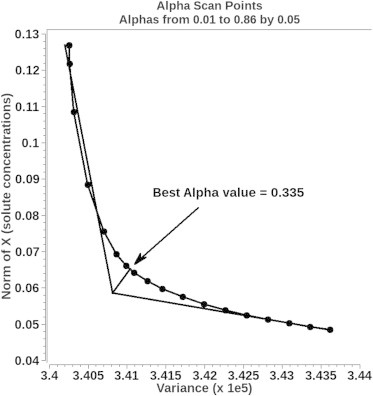
Regularization parameter α determination using the L-curve criterion. The elbow of the curve represents the α-value for the best compromise between variance and norm of the solution. It is found by graphical means through extrapolation from the last five points from either end of the curve. The closest point from the intercept to the curve represents the best-fit α-value.

Materials and Methods

Sedimentation velocity experiments were performed at the Center for Analytical Ultracentrifugation for Macromolecular Assemblies (CAUMA) at the University of Texas Health Science Center at San Antonio (UTHSCSA). All experiments were performed in UV intensity mode, either at 260 or 280 nm in phosphate or TRIS buffers, as indicated. Data were converted to pseudo-absorbance data before fitting, and all RMSD values are reported in absorbance units. All experiments were performed with Epon two-channel centerpieces in an Optima XLI (Beckman Coulter, Brea, CA) at 20°C. Hydrodynamic corrections and partial specific volumes were estimated with the relevant modules for analytes, buffers, and solutions integrated in the software UltraScan-III (UltraScan Project, UTHSCSA, TX). The analysis was performed with UltraScan-III, ver. 2.0, Rel. 1651 (18) according to methods outlined in Demeler (13), and using the PCSA module. All 2DSA, genetic algorithms (GA), and 2DSA/GA Monte Carlo calculations were performed on the XSEDE infrastructure through the UltraScan Science Gateway (19), using the Alamo (UTHSCSA), Lonestar or Stampede (Texas Advanced Computing Center), or Trestles (San Diego Supercomputing Center) clusters. PCSA calculations are sufficiently fast that they can be performed on a modern laptop.

Plasmid pPOL-1-208-12 DNA (20) was prepared as described in Maniatis et al. (21), and depending on fragment sizes needed, either fully or partially digested with Ava-I, Pst-I, or Awl-I. In the experiment shown later in Fig. 7, desired fragments from the partial digest were isolated by preparative 1% agarose gel electrophoresis and mixed at approximately equal proportion (based on absorbance units) with the full plasmid digests. Our plasmid purification did not include a CsCl buoyant density gradient step to avoid introduction of ethidium bromide. This leaves ∼15% of the total absorbance due to chromosomal DNA in the sample, which contributes to a negligible background after digestion. All DNA samples were purified by HPLC using an GE HiTrap Q HP anion exchange column (GE Healthcare Life Sciences, Pittsburgh, PA), and using a 10 mM NaPO₄ buffer, pH 7.5, with a NaCl gradient ranging from 0 to 1.2 M. The desired DNA fragments eluted at ∼660 mM NaCl concentration. HPLC-purified DNA solutions were dialyzed against 1.7 mM sodium phosphate buffer, pH 7.5. Bovine brain clathrin was purified from bovine brain clathrin-coated vesicles as described previously in Morgan et al. (22). Clathrin cages were prepared by dialysis of 0.8 mg/mL bovine brain clathrin into 10 mM Mes pH 6.2, 2 mM CaCl₂ for 7 h.

Figure 7.

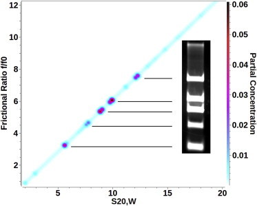
DNA digestion with six fragments as analyzed with the straight-line PCSA parameterization. The DNA fragments resolved by PCSA show excellent correspondence with the 1% agarose gel electrophoresis result, both in position as in partial concentration. To see this figure in color, go online.

Simulation Settings

All fibrinogen simulations were calculated with a Lamm equation solution based on the finite-element method proposed by Claverie et al. (23) with a constant time grid and a regular radial grid containing 10,000 radial points. The simulated solution was interpolated onto a radial grid with 0.001 cm spacing. The same solution was used earlier as a reference solution for determining the accuracy of the ASTFEM solution (8,9). The simulations of the testing data were performed at 1.0 absorbance units with 0.5% random Gaussian distributed noise added, which is equivalent to the noise typically observed in a well-tuned XLA centrifuge (Beckman Coulter) at 280 nm when optical density is <1.0 absorbance units. Each experiment was simulated with 50 equally spaced scans, such that the moving boundary spanned the entire solution column. The meniscus position was fixed at 5.8 cm and the bottom of the cell position was held fixed at 7.2 cm for all simulations. The fibrinogen oligomer mixture was simulated at 20, 40, and 60 krpm (with ω²t at the end of the run ranging between 1.89 × 10¹¹–2.78 × 10¹¹). Simulation of rotor acceleration was applied during the finite-element calculation for each data set. Density and viscosity of the solution was assumed to be that of water at 20°C (0.998234 g/mL, 1.001940 cp).

Results and Discussion

To test the PCSA algorithm, we evaluated the method’s performance on simulated and experimental data containing selected systems in various states of polymerization where heterogeneity in anisotropy and mass was expected. Simulated data will test the method’s ability to recover known parameters from the simulation. The data are simulated with noise contributions equivalent to that found in actual experiments. We chose to simulate five oligomers of fibrinogen (monomer-pentamer) offering heterogeneity in mass and anisotropy. A crystal structure is available (3GHG in the RCSB protein database (24)) which we modeled into oligomeric structures, whose hydrodynamic parameters were predicted using UltraScan-SOMO (25,26) (see Table S2).

We analyzed the simulated data with Monte Carlo methods for genetic algorithms (GA), PCSA with increasing sigmoids (IS), and PCSA with horizontal-line (HL) functional forms. Detailed results comparing the performance of each method for a 40 krpm and a 60 krpm simulation are shown in Table S3. These results show that the GA method performs best, with an average deviation of 3.62% from the simulated parameters, whereas the PCSA-IS method showed a twofold higher deviation of 7.13%, followed by the PCSA-HL with an error rate of 19.73%, which is greater than fivefold worse than the GA method. RMSD values closely followed this pattern, with an average increase of 0.1797% over the simulated RMSD for the GA analysis, 0.4006% for the PCSA-IS, and 2.6996% for the PCSA-HL analysis. All five species were correctly identified in the 40- and 60-krpm data, although the resolution was insufficient to resolve the tetramer from the pentamer, the most closely spaced species, in the 20 krpm data by all methods.

The first experimental system measured the polymerization of clathrin triskelia monomers into fully formed clathrin cages. Due to the monomeric triskelion shape, a large frictional coefficient is expected for the monomeric clathrin triskelia and any incomplete clathrin cages, whereas fully formed cages are expected to be spherical with a frictional ratio approaching unity. Indeed, unconstrained 2DSA analysis suggests the presence of these species (see Fig. 4 A). The pattern in the 2DSA suggests that the two-dimensional grid can be approximated with a decaying exponential or decreasing sigmoidal functional form. As shown in Fig. 4 B, a decreasing sigmoidal parameterization results in an excellent fit (see Fig. 4 C), with an RMSD equivalent to the RMSD from the unconstrained 2DSA fit (0.005467 vs. 0.005437, respectively). The BFM obtained in this fit, while constrained to a single line, closely tracked the s versus f/f₀ distribution of signal observed in the 2DSA, and the multiple split peaks observed in the 2DSA for the low-molecular-weight species can be equally well represented by a single peak with a minor shoulder in the PCSA (Fig. 4 B). A PCSA-HL analysis without regularization over the same parameter range resulted in an increased RMSD of 0.005617 and a uniform frictional ratio of 2.73, far from the more spherical anisotropy expected for the fully formed clathrin cages. The increased RMSD indicates that the heterogeneity in anisotropy contributes a detectable signal above the background noise level to the boundary shape.

Figure 4.

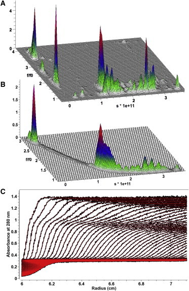
Sedimentation velocity analysis of polymerizing clathrin triskelia in a clathrin assembly reaction. (A) Two-dimensional spectrum analysis. At low sedimentation coefficients, highly anisotropic triskelia monomers and dimers, as well as incompletely formed clathrin cage fragments are apparent, whereas at higher sedimentation coefficients the more spherical, fully formed cages are apparent. (B) Parametrically constrained spectrum analysis of the same data as shown in panel A using a decreasing sigmoidal functional form. The frictional ratio versus sedimentation coefficient distribution observed mirrors the information observed in the 2DSA analysis, but all values are constrained to a single sedimentation-frictional ratio pair. (C) Experimental data (black) overlaid with the fitted PCSA solution (red) for the clathrin assembly reaction mixture. The data demonstrate a near-perfect fit. The PCSA analysis resulted in a BFM with an RMSD of 5.469 × 10⁻³, whereas the unconstrained 2DSA-Monte Carlo analysis resulted in a lower RMSD of 5.437 × 10⁻³.

In the next experiment, a DNA mixture consisting of two double-stranded fragments with sizes 208 and 2812 bp in length was measured. This experiment was repeated under a range of ionic conditions using a 1-mM sodium phosphate buffer containing 1.7, 5, 7, 10, 20, 50, and 150 mM NaCl. When the ionic strength is increased, DNA is expected to exhibit a reduced anisotropy due to increasing charge neutralization along the backbone. As a consequence, the parameterization for each salt concentration describing the anisotropy as a function of DNA fragment length is expected to vary in a systematic fashion. 2DSA analysis of these samples revealed two major species for each salt concentration, with significantly different anisotropies (see Table 1). From this analysis, it can be seen that the confidence intervals are very narrow in the sedimentation domain, but are significantly larger in the frictional domain, especially for the larger component. It is evident that the 2DSA and genetic algorithm Monte Carlo analysis identify many species with the same sedimentation coefficient, but a large range of frictional ratios (see Fig. 2 B). In such a case, the benefit of additional constraints that provide a univalued relationship between sedimentation and anisotropy could be helpful. Because any two species can be fitted with a straight line, a straight-line functional form was chosen to represent these samples in the PCSA. The fits of these experiments by straight-line PCSA are shown in Fig. 5. They reveal a striking relationship between the slope of the straight-line parameterization and the salt concentration, clearly showing a systematic decrease in anisotropy with increasing salt concentration (see Fig. 6).

Table 1.

2DSA-Monte Carlo results for all examined salt concentrations

[NaCl] (mM)	s [1]	f/f0 [1]	% [1]	s [2]	f/f0 [2]	% [2]
1.7	5.14 (4.76 5.52)	3.88 (3.17, 4.58)	43.1	10.68 (10.46, 10.91)	12.04 (3.13, 20.96)	31.5
5.0	5.30 (5.07 5.52)	3.83 (3.01, 4.65)	43.2	11.12 (10.26, 11.99)	9.91 (8.64, 11.18)	25.9
7.0	5.40 (4.87 5.92)	3.71 (2.74, 4.68)	42.9	11.35 (11.16, 11.54)	10.17 (8.30, 12.04)	28.2
10.0	5.44 (4.98 5.90)	3.74 (2.40, 5.08)	42.3	11.42 (11.10, 11.74)	10.45 (6.34, 14.56)	34.3
20.0	5.56 (5.32 5.79)	3.42 (2.48, 4.35)	42.5	11.67 (11.45, 11.89)	10.78 (7.98, 13.57)	35.5
50.0	5.65 (5.13 6.18)	3.32 (1.49, 5.16)	43.4	11.93 (11.25, 12.60)	9.95 (3.69, 16.21)	30.2
150.0	5.60 (5.28 5.92)	3.44 (1.92, 4.95)	42.4	12.03 (11.44, 12.63)	9.21 (5.40, 13.03)	31.4

Ninety-five percent confidence limits are shown in parentheses. Numbers in square brackets refer to the fragment number in the DNA mixture. All values are corrected for conditions equivalent to water at 20°C.

Figure 5.

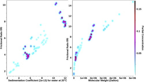
PCSA analysis of a mixture of two linear dsDNA fragments in 1, 5, 7, 10, 20, 50, and 150 mM NaCl using a straight-line function. Lower salt concentration results in a steeper slope, indicating a higher anisotropy. The dependence of the slope on salt concentration is shown in Fig. 6. To see this figure in color, go online.

Figure 6.

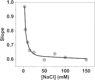
Dependence of the PCSA-SL slope parameter on the salt concentration used for DNA. A strong decrease in slope is apparent up to 30 mM NaCl, suggesting maximum flexibility reached in the DNA conformation at 30 mM NaCl.

As in the previous example, the RMSD values of the PCSA fits are nearly indistinguishable from the RMSD values obtained from the 2DSA or GA fits, as are the locations of the major species in the two-dimensional grid identified by either method. There are also a number of minor species apparent (light cyan color, each with <2% of the total concentration) in all samples, which presumably result from low-concentration digestion products of remaining chromosomal DNA. Due to their low concentration, the confidence in their position is also very low and they do not appear necessarily at the same positions when analyzed under different salt conditions. A detailed comparison of results between all methods and parameterizations in the PCSA for the sedimentation velocity experiment of 1.7 mM NaCl DNA mixture is shown in Table 2.

Table 2.

Comparison of results from different analysis methods for a sedimentation velocity experiment of a DNA mixture consisting of two double-stranded fragments in 1.7 mM NaCl

Monte Carlo	s [1]	f/f0 [1]	% [1]	s [2]	f/f0 [2]	% [2]	RMSD
2DSA	5.14 (4.74, 5.74)	3.87 (3.11, 4.63)	43.5	10.67 (10.21, 11.13)	12.67 (1.71, 23.63)	35.4	3.2146
GA	5.15 (5.12, 5.18)	3.71 (3.45, 3.97)	46.7	10.66 (10.64, 10.68)	11.25 (10.10, 12.39)	35.3	3.2609
IS	5.16 (4.56, 5.77)	3.74 (3.21, 4.27)	49.6	10.67 (10.26, 11.08)	11.01 (10.38, 11.65)	38.7	3.3697
SL	5.05 (4.55, 5.55)	3.95 (3.25, 4.65)	44.6	10.67 (9.97, 11.38)	9.74 (9.02, 10.46)	40.2	3.4253
HL	5.22 (1.44, 9.00)	7.20 (0.00, 0.00)	50.4	10.71 (9.84, 11.58)	7.20 (0.00, 0.00)	43.1	4.6832

One-hundred iteration Monte Carlo analyses were performed on 2DSA, genetic algorithms (GA), PCSA with an increasing sigmoid function (IS), straight-line parameterization (SL), and horizontal-line parameterization (HL). Ninety-five percent confidence limits are shown in parentheses. Numbers in square brackets refer to the fragment number in the DNA mixture. All values are corrected for conditions equivalent to water at 20°C. Two-dimensional pseudo-three-dimensional plots of each analysis are shown in Fig. S3, Fig. S4, Fig. S5, Fig. S6, and Fig. S7 in the Supporting Material. A large increase in RMSD is seen when PCSA-HL parameterization is used (compare also Fig. S2).

This comparison highlights several important trends:

• 1.The 2DSA results in the best RMSD and also in the broadest confidence region for the frictional ratio, especially for the larger component. The lowest RMSD can be explained by the degeneracy of the method, where even low-amplitude stochastic noise contributions are fitted. The broad confidence interval in the frictional ratio can be explained by the limited diffusion information available for the fastest sedimenting species, which is already low due to the high anisotropy of the large DNA fragment. However, the value of the imposed constraints (both by the PCSA as well as by the GA) is clear: The confidence region is substantially reduced when parameterization or parsimonious regularization is used, without resulting in a significant penalty in RMSD.
• 2.Frictional ratios are in good agreement for all methods except the horizontal-line (HL) parameterization, which reports a weight average frictional ratio only, and therefore by definition misses the true frictional ratio values, and also suffers from a substantial increase in RMSD. The best agreement is obtained for the smaller species due to slower sedimentation and faster diffusion (except for the HL parameterization).
• 3.RMSD values are very similar, with a small increase in RMSD apparent when additional constraints are imposed. The RMSD order observed is 2DSA < GA < PCSA-IS < PCSA-SL ≪ PCSA-HL. These constraints are derived either from parsimonious regularization (in the GA) or from the parameterization in the PCSA. When the parameterization is no longer able to capture the information content present in the data, the RMSD jumps to much larger values, as is observed in the PCSA-HL parameterization.
• 4.All methods produce very similar sedimentation coefficients, although the results from the PCSA-HL method deviates from all other methods, and suffers from overly broad confidence intervals in the smaller species, and in additional species not identified in the other methods (Fig. 2 C).

This is explained by the following observation: When the straight-line model is restricted to zero slope, the parameterization is identical to the parameterization used in the C(s) analysis (10). Such a parameterization produces a very different and incorrect result and returns a significantly elevated RMSD (see Table 2). Moreover, the sedimenting species corresponding to the smaller DNA fragment is now split into multiple false-positive species (Fig. 2, C–E). In addition, because the frictional ratio represents a weight average, and is needed for an absolute molecular weight transformation, any derived molecular weights for any species will more than likely be incorrect. Regularization does not alleviate this problem; it merely hides it by artificially broadening the width of the peak of the smaller species (see Fig. 2 C). Choosing the α-value suggested by the L-curve criterion during Tikhonov regularization simply smoothens the solution without eliminating the false-positive solutes (Fig. 2 C). We believe that this outcome is an artifact in the PCSA-HL parameterization stemming from its inability to accommodate heterogeneity in anisotropy, and the least-squares optimization.

When a BFM is obtained with the HL parameterization for a sample with heterogeneity in anisotropy, the resulting f/f₀ value represents a weight average of all species in the system, which by definition has to be higher than the f/f₀ of the most globular species in the mixture. Any Lamm equation solution of such a species will have a steeper boundary than one for the actual species, causing a large RMSD in the final fit. However, during least-squares minimization a solution with a lower RMSD that also maintains the weight average f/f₀ can be found by introducing multiple false-positive species with smaller amplitudes in the vicinity of the actual species, considerably broadening the peak width (see Fig. 2, D and E, for comparison), but better satisfying the least-squares condition. Increasing the regularization parameter beyond the L-curve criterion in an attempt to join the false-positive species into a single peak, centered around the desired species, increases the RMSD further and causes nonrandom residuals (see Fig. S2 in the Supporting Material). Monte Carlo analysis of the sedimentation coefficient error intervals around both species using 2DSA, GA, or PCSA analysis demonstrates that the peak width should be much more narrow than the regularized HL parameterization would suggest. This demonstrates that fitting of samples with heterogeneity in anisotropy using PCSA-HL, with or without regularization, may unfavorably impact the resolution and peak width of actual species, and may introduce false-positive species.

When a finite-element model for an experiment provides random residuals, and allows for heterogeneity in anisotropy, a transformation of the sedimentation coefficient distribution to absolute molecular weight should be possible, provided an accurate partial specific volume is available. As can be seen in Fig. 5, a transformation of the sedimentation coefficient distributions from the seven salt concentrations clearly shows that the molecular weights for the two DNA species are not identical, and instead show a consistent shift to larger molecular weights for lower salt concentrations (Fig. 5, right panel). This discrepancy could be explained by the primary charge effect or a salt-dependent change in hydration of DNA, which causes the partial specific volume value to change, affecting the molecular-weight transformation. However, in our analysis, we assumed a constant PSV of 0.55 mL/mg for all salt concentrations.

The final experimental example shows a DNA restriction digest dissolved in 100 mM NaCl containing phosphate buffer, giving rise to a mixture of 5 dsDNA fragments. A straight line (Fig. 7) and increasing sigmoidal functional form (see Fig. S8) was used in the PCSA to fit the data. When comparing the two-dimensional sedimentation pattern of a straight-line functional form to a 1% agarose gel electrophoresis image of the same DNA mixture, a remarkable resolution and agreement with the bands of the gel image are achieved, where the solutes identified by the PCSA mirror closely the spacing and relative concentration of each species seen in the gel image. Also, the slope derived from the straight-line fit is 0.65, in good agreement with the slope predicted for the 100-mM NaCl concentration in the previous experiment (Fig. 6). The result suggests that both functional forms are similarly appropriate for this system.

Conclusion

We have presented a method that effectively searches the two-dimensional solution space over s and f/f₀ by constraining the solution to a single-valued functional form, which assures that the solution does not contain sedimenting species with multiple frictional coefficients. In summary, these results demonstrate that the PCSA offers an excellent mechanism for constraining the 2DSA solution to a single-valued function without sacrificing the generality of heterogeneity in anisotropy, and can provide useful information about the intrinsic anisotropic properties of a system, and elucidate trends such as anisotropy changes in response to an external perturbation such as salt concentration. At the same time, our method does not require the user to apply unwarranted constraints demanding constant frictional ratios for the entire solution as is done in the C(s) method and the horizontal-line parameterization. Simulated data also showed that the PCSA-IS method, which allows for variation in the frictional ratio, performs significantly better and provides higher accuracy than the PCSA-HL when fitting systems that exhibit heterogeneity in size and anisotropy.

We showed that the PCSA method with appropriate functional forms can provide useful parameterizations for anisotropies of polymer growth, and allows prediction of intermediate values for polymer size distributions. The PCSA provides a generalized solution that allows for heterogeneity in anisotropy and size, while still providing a univalued function.

References

- 1.Lamm O. The differential equation of ultracentrifugation [Die Differentialgleichung der Ultrazentrifugierung] Ark. Mat. Astron. Fys. 1929;21B:1–4. [Google Scholar]
- 2.Demeler B., Brookes E.H., Kim C.A. Characterization of reversible associations by sedimentation velocity with ULTRASCAN. Macromol. Biosci. 2010;10:775–782. doi: 10.1002/mabi.200900481. [DOI] [PubMed] [Google Scholar]
- 3.Brookes, E. H., Boppana, R. V., and Demeler, B. 2006. Computing large sparse multivariate optimization problems with an application in biophysics. Supercomputing ‘06 ACM. 0–7695–2700–0/06.
- 4.Brookes E.H., Cao W., Demeler B. A two-dimensional spectrum analysis for sedimentation velocity experiments of mixtures with heterogeneity in molecular weight and shape. Eur. Biophys. J. 2010;39:405–414. doi: 10.1007/s00249-009-0413-5. [DOI] [PubMed] [Google Scholar]
- 5.Lawson C.L., Hanson R.J. Prentice-Hall; Englewood Cliffs, NJ: 1974. Solving Least Squares Problems. [Google Scholar]
- 6.Brookes, E. H., and B. Demeler. 2007. Parsimonious regularization using genetic algorithms applied to the analysis of analytical ultracentrifugation experiments. GECCO Proc. ACM. 978–1-59593–697–4/07/0007.
- 7.Demeler B., Brookes E.H. Monte Carlo analysis of sedimentation experiments. Colloid Polym. Sci. 2008;286:129–137. [Google Scholar]
- 8.Cao W., Demeler B. Modeling analytical ultracentrifugation experiments with an adaptive space-time finite element solution of the Lamm equation. Biophys. J. 2005;89:1589–1602. doi: 10.1529/biophysj.105.061135. [DOI] [PMC free article] [PubMed] [Google Scholar]
- 9.Cao W., Demeler B. Modeling analytical ultracentrifugation experiments with an adaptive space-time finite element solution for multicomponent reacting systems. Biophys. J. 2008;95:54–65. doi: 10.1529/biophysj.107.123950. [DOI] [PMC free article] [PubMed] [Google Scholar]
- 10.Schuck P. Size-distribution analysis of macromolecules by sedimentation velocity ultracentrifugation and Lamm equation modeling. Biophys. J. 2000;78:1606–1619. doi: 10.1016/S0006-3495(00)76713-0. [DOI] [PMC free article] [PubMed] [Google Scholar]
- 11.Levenberg K. A Method for the solution of certain non-linear problems in least squares. Q. Appl. Math. 1944;2:164–168. [Google Scholar]
- 12.Marquardt D. An algorithm for least-squares estimation of nonlinear parameters. SIAM J. Appl. Math. 1963;11:431–441. [Google Scholar]
- 13.Demeler B. Methods for the design and analysis of sedimentation velocity and sedimentation equilibrium experiments with proteins. Cur. Protoc. Prot. Sci. 2010;Chapt. 7 doi: 10.1002/0471140864.ps0713s60. Unit 7-13. [DOI] [PMC free article] [PubMed] [Google Scholar]
- 14.Demeler B., van Holde K.E. Sedimentation velocity analysis of highly heterogeneous systems. Anal. Biochem. 2004;335:279–288. doi: 10.1016/j.ab.2004.08.039. [DOI] [PubMed] [Google Scholar]
- 15.Aster R.C., Borchers B., Thurber C.H. Elsevier Academic Press; New York: 2005. Parameter Estimation and Inverse Problems. [Google Scholar]
- 16.Hansen P.C. Analysis of discrete ill-posed problems by means of the L-curve. SIAM Rev. 1992;34:561–580. [Google Scholar]
- 17.Box G.E.P., Muller M.E. A note on the generation of random normal deviates. Ann. Math. Stat. 1958;29:610–611. [Google Scholar]
- 18.Demeler, B., G. Gorbet, …, B. Dubbs. 2013. ULTRASCAN-III Ver. 2.0: a comprehensive data analysis software package for analytical ultracentrifugation experiments. http://www.ultrascan3.uthscsa.edu/.
- 19.The Extreme Science and Engineering Discovery Environment (XSEDE) Scientific Gateway Portal, National Science Foundation, Arlington, VA. https://www.xsede.org/gateways-listing.
- 20.Georgel P., Demeler B., van Holde K.E. Binding of the RNA polymerase I transcription complex to its promoter can modify positioning of downstream nucleosomes assembled in vitro. J. Biol. Chem. 1993;268:1947–1954. [PubMed] [Google Scholar]
- 21.Maniatis T., Fritsch E.F., Sambrook J. A Laboratory Manual. Cold Spring Harbor Laboratory; New York: 1982. Molecular Cloning. [Google Scholar]
- 22.Morgan J.R., Zhao X., Lafer E.M. A role for the clathrin assembly domain of AP180 in synaptic vesicle endocytosis. J. Neurosci. 1999;19:10201–10212. doi: 10.1523/JNEUROSCI.19-23-10201.1999. [DOI] [PMC free article] [PubMed] [Google Scholar]
- 23.Claverie J.M., Dreux H., Cohen R. Sedimentation of generalized systems of interacting particles. I. Solution of systems of complete Lamm equations. Biopolymers. 1975;14:1685–1700. doi: 10.1002/bip.1975.360140811. [DOI] [PubMed] [Google Scholar]
- 24.Kollman J.M., Pandi L., Doolittle R.F. Crystal structure of human fibrinogen. Biochemistry. 2009;48:3877–3886. doi: 10.1021/bi802205g. [DOI] [PubMed] [Google Scholar]
- 25.Brookes E.H., Demeler B., Rocco M. The implementation of SOMO (SOlution MOdeller) in the ULTRASCAN analytical ultracentrifugation data analysis suite: enhanced capabilities allow the reliable hydrodynamic modeling of virtually any kind of biomacromolecule. Eur. Biophys. J. 2010;39:423–435. doi: 10.1007/s00249-009-0418-0. [DOI] [PMC free article] [PubMed] [Google Scholar]
- 26.Brookes E.H., Demeler B., Rocco M. Developments in the US-SOMO bead modeling suite: new features in the direct residue-to-bead method, improved grid routines, and influence of accessible surface area screening. Macromol. Biosci. 2010;10:746–753. doi: 10.1002/mabi.200900474. [DOI] [PubMed] [Google Scholar]
Associated Data
This section collects any data citations, data availability statements, or supplementary materials included in this article.