Chromatin Hydrodynamics

Abstract

Following recent observations of large scale correlated motion of chromatin inside the nuclei of live differentiated cells, we present a hydrodynamic theory—the two-fluid model—in which the content of a nucleus is described as a chromatin solution with the nucleoplasm playing the role of the solvent and the chromatin fiber that of a solute. This system is subject to both passive thermal fluctuations and active scalar and vector events that are associated with free energy consumption, such as ATP hydrolysis. Scalar events drive the longitudinal viscoelastic modes (where the chromatin fiber moves relative to the solvent) while vector events generate the transverse modes (where the chromatin fiber moves together with the solvent). Using linear response methods, we derive explicit expressions for the response functions that connect the chromatin density and velocity correlation functions to the corresponding correlation functions of the active sources and the complex viscoelastic moduli of the chromatin solution. We then derive general expressions for the flow spectral density of the chromatin velocity field. We use the theory to analyze experimental results recently obtained by one of the present authors and her co-workers. We find that the time dependence of the experimental data for both native and ATP-depleted chromatin can be well-fitted using a simple model—the Maxwell fluid—for the complex modulus, although there is some discrepancy in terms of the wavevector dependence. Thermal fluctuations of ATP-depleted cells are predominantly longitudinal. ATP-active cells exhibit intense transverse long wavelength velocity fluctuations driven by force dipoles. Fluctuations with wavenumbers larger than a few inverse microns are dominated by concentration fluctuations with the same spectrum as thermal fluctuations but with increased intensity.

Introduction

Nuclei of living cells are places of intense activity (1). DNA-encoded genes are transcribed into messenger RNA strands by RNA polymerases. Helicases provide access for the RNA polymerases to a DNA molecule by unwinding and unzipping it. Topoisomerases control the supercoiling of DNA. The enzymatic activity is fueled by the consumption of free energy obtained from ATP hydrolysis and from other sources. Chromatin serves as a substrate for this activity. Chromatin is composed of centimeter-long DNA molecules wound around spool-like histone octamers, the nucleosomes, comprising the so-called 10-nm fiber. In the less dense regions of the nucleus, referred to as “euchromatin”, the 10-nm fiber is packed rather loosely, allowing easy access to DNA for DNA-associating proteins. The more densely packed regions are referred to as “heterochromatin”. Genes located inside the heterochromatin regions require local decondensation to allow for gene expression (2). This is facilitated by the covalent modification of the histone proteins through acetylation, methylation, and phosphorylation, which modulates the affinity of nucleosomes for each other. In addition, ATP-consuming chromatin remodeling complexes actively rearrange the positions of nucleosomes (3).

The content of a cell nucleus is quite complex. The chromatin 10-nm fiber described above is immersed in a viscous liquid, the nucleoplasm, which itself has a very rich composition: it contains not only free proteins, nucleotides, RNAs, small molecules and salts, but also nucleoli and subnuclear bodies such as Cajal bodies and paraspeckles or PML bodies. During interphase—the time in the cell cycle between two cell divisions—the content of the nucleus can, to first approximation, be viewed as a rather concentrated and nonuniform chromatin solution in which 10-nm fiber material, a gigantic polymer, is dissolved in a fluid comprised of much smaller molecules. We will refer to this solvent fluid as “nucleoplasm” (thus ignoring the presence of subnuclear bodies). In this chromatin solution, the chromatin fiber itself may have higher levels of organization, such as the (lately much disputed (4,5)) 30-nm fiber.

Chromatin dynamics has been investigated by high-resolution imaging of fluorescently labeled nuclear proteins and single DNA sites. Early work concluded that, during interphase, chromatin underwent constrained (corralled) diffusive motion with typical diffusion constants of the order of 10⁻⁴ μm²/s (6–8). Analysis of three-dimensional tracks of labeled telomeres revealed subdiffusive motion up to timescales of 10–100 s (9). Tracking of labeled lac-operator sites on chromatin showed both ATP and thermally driven dynamics. Long periods of constrained diffusion were observed, followed by short bursts of superdiffusive directed motion (150-nm leaps of ∼1 s). Upon ATP depletion, only localized motion was observed (10). Trajectories of micron-sized microinjected particles (11) were found to be constrained within cages of ∼250 nm size while ATP-dependent subdiffusion of chromosomal loci was observed in bacterial cells and in yeast cells (12). Interphase chromatin of embryonic stem cells was observed to execute ATP-dependent periodic breathing motion on timescales of 0.1–0.01 s, with amplitudes of ∼100 nm (13). This breathing motion is suppressed for differentiated cells while the fraction of condensed chromatin increases. The architectural proteins that maintain the structure of chromatin are hyperdynamic in pluripotent embryonic stem cells but are increasingly immobilized upon differentiation (14).

A microrheology study of the viscoelastic properties of chromatin using 100-nm beads has found predominantly elastic behavior in the frequency range 0.2–5.0 Hz with broadly distributed values of storage and loss moduli (15). Very different values for the moduli were reported in studies of the displacement of a spherical magnetic nanoparticle of 1-μm diameter (16) and the rotation of a cylindrical magnetic nanoparticle of 1.5-μm length and 0.2-μm diameter (17). A macroscopic rheology study using time-dependent deformation of entire cells with fluorescently labeled nuclei has found that nuclei of embryonic stem cells and those of cells lacking A/C lamins were much more deformable than those of differentiated cells (18).

All these studies focused on the tracking of a small number of tracer particles. In a recent study, fluorescently labeled histones were used to map the chromatin movement simultaneously across the entire nucleus (19). The study showed that chromatin motion of human HeLa cells appears to be spatially correlated over length scales ranging from 250 nm to 5 μm. This is a surprising result: individual events such as gene expression, DNA replication, or DNA repair are presumably highly specific so one would not expect large- scale correlations. The aim of this article is to provide a theoretical framework for the analysis of studies of ATP-driven chromatin dynamics. The basic theoretical assumption of the proposed framework is that the velocity fluctuations inside chromatin can be described within linear response theory applied to a viscoelastic two-fluid model.

The response of the chromatin solution to both thermal fluctuations and to active events is determined by the dynamic susceptibility of the two-fluid model. It could be questioned whether a very complex system such as chromatin could be described by any simple theoretical model. Linear hydrodynamic properties of complex systems are in general determined by conservation laws and symmetry. These properties depend on the molecular details of the local structure of the material only insofar as these determine the numerical value of the response moduli of the system. For the case of chromatin, conservation of solvent and conservation of 10-nm fiber material plays such a role. In terms of symmetry, the chromatin solution is treated as a fluid in the sense that the 10-nm fiber is not restrained by any three-dimensional network of covalent cross-links (even if there are higher levels of organization) so the shear modulus at low frequencies should be zero. Moreover, the chromatin solution appears to be relatively isotropic on length scales from tens of nanometers to several microns. We will show that one can similarly classify active events as scalar or vectorial, depending on symmetry considerations.

An important motivation for adopting this methodology was that the hydrodynamic method has been applied with success to active gels such as the actin-myosin system with motor protein activity treated as a distribution of force dipoles. The motor activity produced highly correlated, low-frequency shear fluctuations through coupling to long-wavelength shear modes of the gel. A recent review summarizes studies of soft materials where large-scale cooperativity and hydrodynamic fluctuations are driven by active force dipoles (20).

We propose that a study of the collective dynamics of chromatin might well be relevant to questions concerning gene expression that are of interest to the life-science community. Collective gene expression events can occur as part of the natural progression through the cell cycle or in response to external signaling cues or environmental challenge. Different forms of collective gene expression could generate different active hydrodynamic fluctuation spectra. If that is the case, then the measurement of the flow spectral densities, as described in this article, could provide a new diagnostic tool for probing collective activity in the nucleus.

Theory

Two-fluid model

We start with the specification of the linear hydrodynamics of an idealized chromatin solution that is homogeneous and has no sources of free energy consumption. This passive chromatin solution will be treated as a two-fluid model, a viscoelastic fluid composed of a solvent (i.e., the nucleoplasm) and a polymeric material (i.e., the chromatin fiber). The chromatin solution is assumed to have an accessible state of thermodynamic equilibrium with no osmotic or hydrodynamic pressure gradients. Chromatin itself is quite compressible: a change in volume fraction of the chromatin fiber in some region can be compensated by solvent (nucleoplasm) flow in or out of that region. The combined solution composed of polymers (chromatin fiber) plus solvent (nucleoplasm), however, will be treated as incompressible. The polymer volume fraction in this equilibrium state will be denoted by ϕ₀. Deviations from this equilibrium state are described by the following set of collective hydrodynamic variables:

• 1.Solvent flow velocity ${\overrightarrow{v}}^s$;
• 2.Polymer flow velocity ${\overrightarrow{v}}^p$;
• 3.Deviation of polymer volume fraction from equilibrium δϕ;
• 4.Hydrodynamic pressure P; and
• 5.Osmotic pressure Π.

The linearized hydrodynamic equations of a two-fluid model (21) read as

$$\zeta \left({\overrightarrow{v}}^p-{\overrightarrow{v}}^s\right)=\overrightarrow{\nabla }\cdot \overleftrightarrow{\sigma }-\overrightarrow{\nabla }\text{Π}-{\varphi }_0\overrightarrow{\nabla }P,$$ (1)

$$\zeta \left({\overrightarrow{v}}^s-{\overrightarrow{v}}^p\right)=-\left(1-{\varphi }_0\right)\overrightarrow{\nabla }P.$$ (2)

The derivation of these equations, based on general principles of linear response theory (see, e.g., Landau and Lifschitz (22) or Doi (23)) is summarized in Section S1 in the Supporting Material. Equation 1 relates the viscous drag exerted by the solvent on the chromatin polymer to the force per unit volume due to polymer-polymer interactions (first two terms) plus the hydrodynamic force per unit volume exerted on the polymer. The expression ζ ∼ η₀/ξ² is the inverse of the solvent permeability of chromatin with η₀ the viscosity of the solvent and ξ the typical size of the pores of the chromatin. Next, $\overleftrightarrow{\sigma }$ is the (traceless) shear stress tensor of chromatin that is additional to the separately included (minus) gradient of the osmotic pressure Π. Equation 2 relates the viscous drag exerted by the polymers on the solvent with the hydrodynamic force per unit volume exerted on the solvent volume fraction (Darcy’s law for porous media); this treatment neglects viscous stresses in the solvent on length scales larger than the mesh size (see Milner (24) for further details). Finally, osmotic pressure variations are related to concentration variations by Π = Kδϕ with K the osmotic modulus of the polymer system.

The hydrodynamics of chromatin will be assumed to be that of a generalized, linear, non-Newtonian, viscoelastic fluid. For such fluids, the shear stress tensor can be expressed as

$$i{q}_i{\sigma }_{ij}\left(\overrightarrow{q},\omega \right)=-E\left(q,\omega \right)\left(\frac{1}{3}{q}_j{q}_i{v}_i^p+q^2{v}_j^p\right).$$ (3)

Here, E(q,ω) is a generalized complex shear viscosity of chromatin that depends on both wavevector and frequency. We will not specify the form of E(q,ω), which must be provided either by microrheological experiments or by a microscopic theory of the chromatin solution. E(q,ω) is related to the more familiar complex modulus by G(q,ω) = −iωE (q,w).

Our convention for the Fourier transforms in this expression is

$$\varphi \left(\overrightarrow{q},\omega \right)=\underset{\Delta V}{\int }\underset{-\infty }{\overset{\infty }{\int }}\varphi \left(\overrightarrow{r},t\right)e^{i\left(\omega t-\overrightarrow{q}\cdot \overrightarrow{r}\right)}d\overrightarrow{r}dt,$$ (4a)

$$\varphi \left(\overrightarrow{r},t\right)=\frac{1}{\Delta V}\sum _{\overrightarrow{q}}\underset{-\infty }{\overset{\infty }{\int }}\varphi \left(\overrightarrow{q},\omega \right)e^{i\left(-\omega t+\overrightarrow{q}\cdot \overrightarrow{r}\right)}\frac{d\omega }{2\pi },$$ (4b)

and treated similarly for the other fields. The value ΔV is nucleus volume. Wavevector and frequency are limited by the fact that q/2π must be large compared to the inverse of the size of the nucleus and ω/2π must be large compared to the inverse of the duration of the interphase stage.

The condition that the full system of solvent plus chromatin is incompressible can be expressed as

$$\overrightarrow{\nabla }\cdot \left[\left(1-{\varphi }_0\right){\overrightarrow{v}}^s+{\varphi }_0{\overrightarrow{v}}^p\right]=0,$$ (5)

while the linearized continuity equation for polymer material is

$$\partial \varphi /\partial t+{\varphi }_0\overrightarrow{\nabla }\cdot {\overrightarrow{v}}^p=0\text{.}$$ (6)

This completes the hydrodynamic description of passive chromatin as a linear non-Newtonian, viscoelastic fluid. The next step is a description of the active sources. We start with so-called scalar events.

Scalar activity

Activity associated with the local condensation or decondensation of chromatin driven by free energy consumption is termed a “scalar event”. Unlike the active force dipoles of the actin-myosin system mentioned in the Introduction, scalar activity is nondirectional. Thermal concentration fluctuations are explicitly excluded from the definition of scalar events. Fig. 1 shows schematically an example of a scalar event.

Figure 1.

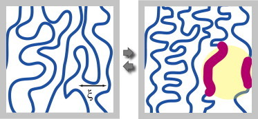
Example of a scalar event. (Left panel) Equilibrium state of chromatin. The length scale ξ indicates the average spacing between adjacent sections of the 10-nm fiber. (Right panel, yellow region) Localized region where 10-nm fiber has been chemically altered, with respect to the equilibrium state, by (de)acetylation and/or (de)methylation of the histones. Sections of the 10-nm fiber that have been chemically altered are shown (red). Neither the nucleosomes nor the enzymes that produce the alterations are shown. The chemical alteration causes a local change in the solubility of the 10-nm fiber, causing influx or efflux of solvent. (Also in right panel) Increased solubility of localized decondensation of the chromatin. (Gray arrows) These changes are reversible. (Gray frame) Field of view. To see this figure in color, go online.

The shift is assumed to be due to a number of isolated events at different sites of the chromatin. In Section S1 in the Supporting Material, it is shown that, in linear response theory, scalar activity can be included as a shift in the osmotic pressure of the form

$$\text{Π}\left(\overrightarrow{r},t\right)=K\delta \varphi \left(\overrightarrow{r},t\right)-\alpha \left(\overrightarrow{r},t\right),$$

where

$$\alpha \left(\overrightarrow{r},t\right)=\sum _k{s}_k\delta \left(\overrightarrow{r}-{\overrightarrow{R}}_k\right)g\left(t-t_k\right)$$ (7)

is the activity function. Here, s_k indicates the sign and strength of the condensation or decondensation event at location ${\overrightarrow{R}}_k$ at some time t_k. The dimensionless function g(t) is zero for negative arguments whereas for positive arguments it decays with time. A simple choice for g(t) would be

$$\theta \left(t\right)\text{exp}\left(-t/{\tau }_a\right),$$

with τ_a the typical duration of such an event and θ(t) the step function, which equals 1 for positive arguments and 0 for negative arguments.

Single scalar event

Assume that only one scalar event takes place, at the origin at time t = 0. The linearized force-balance equation is then

$$\zeta \left({\overrightarrow{v}}^p-{\overrightarrow{v}}^s\right)=\overrightarrow{\nabla }\overleftrightarrow{\sigma }-K\overrightarrow{\nabla }\delta \varphi -{\varphi }_0\overrightarrow{\nabla }P+s\overrightarrow{\nabla }\delta \left(\overrightarrow{r}\right)g\left(t\right).$$ (8)

In a few lines of algebra, this yields

$$\frac{\partial \delta \varphi }{\partial t}=D{\nabla }^2\delta \varphi -\tilde{s}{\nabla }^2\delta \left(\overrightarrow{r}\right)g\left(t\right)-\frac{{\left(1-{\varphi }_0\right)}^2}{\zeta /{\varphi }_0}\overrightarrow{\nabla }\cdot \left(\overrightarrow{\nabla }\overleftrightarrow{\sigma }\right),$$ (9)

with

$$D=K\frac{{\left(1-{\varphi }_0\right)}^2}{\zeta /{\varphi }_0}$$

and

$$\tilde{s}=s\frac{{\left(1-{\varphi }_0\right)}^2}{\zeta /{\varphi }_0}.$$

We can identify D as a collective diffusion constant. This equation can be viewed as defining a Green’s function for scalar events. In Section S2 in the Supporting Material, we solve this equation for the special case of a Newtonian fluid. It is found to describe a localized change in polymer concentration at the origin plus a transient collective diffusion pulse that travels radially outwards from the origin. The volume integral over the concentration variation is 0: no new material is introduced by the localized change in solubility.

Distributed scalar events

For the general case of a spatial and temporal distribution of scalar events, the concentration profile induced by the scalar events can be shown to be given by the linear response equation

$$\delta \varphi \left(\overrightarrow{q},\omega \right)=\chi \left(q,\omega \right)\alpha \left(\overrightarrow{q},\omega \right),$$ (10)

where

$$\chi \left(q,\omega \right)=\frac{i{q}^2{\varphi }_0}{\omega \left[\frac{\zeta }{{\left(1-{\varphi }_0\right)}^2}+\frac{4}{3}E\left(q,\omega \right)q^2\right]+i{q}^{2}K{\varphi }_0}$$ (11)

is the dynamic susceptibility; see Section S3 in the Supporting Material for the derivation. In the limit of zero frequency, χ(q,ω = 0) reduces to the static osmotic susceptibility 1/K. The dynamic susceptibility has pole singularities in the lower-half of the complex frequency plane that correspond to the collective modes of the system. In Section S7 in the Supporting Material, as a matter of a mathematical example, we work out the calculations for the artificial case when passive chromatin is assumed to have the rheological properties of the Maxwell fluid. Two collective modes are present in that case, corresponding to hybridized collective diffusion and stress relaxation.

Ensemble averaging of scalar events

Assume a sequence of scalar events is observed, e.g., the initiation or termination of the expression of a specific sequence of genes, DNA replication, or repair, etc. Because only a limited amount of data may be obtainable in a particular experiment on a given cell, strong statistical variations are to be expected. To reduce the effect of statistical variability, the experiment could be repeated for different cells at the same stage of the cell cycle and under the same stimulus conditions. The magnitude of the ensemble-averaged source activity $\langle \alpha \left(\overrightarrow{q},\omega \right)\rangle$ then depends on the degree of correlation between different cells. If this ensemble average is nonzero, then according to the linear response theory there should be a nonzero ensemble-averaged longitudinal flow velocity pattern of the form

$$\langle v_{\parallel }^p\left(\overrightarrow{q},\omega \right)\rangle =\frac{\omega }{{\varphi }_{0}q}\chi \left(q,\omega \right)\langle \alpha \left(\overrightarrow{q},\omega \right)\rangle .$$ (12)

On the other hand, if $\langle \alpha \left(\overrightarrow{q},\omega \right)\rangle$ averages to zero due to lack of correlation, one can still measure the ensemble-averaged second moment of the velocity fluctuations.

Assume an ensemble of cell nuclei at the same stage of the cell cycle and under the same external conditions for the case that gene expression is highly stochastic so that after ensemble averaging, the first moment is $\langle \alpha \left(\overrightarrow{q},\omega \right)\rangle$ = 0. If active events are locally correlated in space and in time, then the correlation should depend mainly on the time difference t − t′ between events—assumed small compared with the characteristic timescale of the cell cycle—and on the distance $\overrightarrow{r}-{\overrightarrow{r}}^{\prime }$ between events, assuming neither $\overrightarrow{r}$ nor ${\overrightarrow{r}}^{\prime }$ are located close to the nuclear envelope. The second moment for stochastic active scalar events is defined as

$$\langle \alpha \left(\overrightarrow{q},\omega \right){\alpha }^{\text{∗}}\left({\overrightarrow{q}}^{\prime },{\omega }^{\prime }\right)\rangle =\Delta T\Delta V{\left({\alpha }^2\right)}_{\overrightarrow{q},\omega }{\delta }_{\omega ,{\omega }^{\prime }}{\delta }_{\overrightarrow{q},{\overrightarrow{q}}^{\prime }},$$ (13)

where the asterisk denotes complex conjugation. Wavevectors are discretized in the usual way by boundary conditions imposed at the surface of the volume ΔV of the nucleus (which do not need to be specified for q ≫ 1/ΔV^1/3). The Kronecker delta notation ${\delta }_{\overrightarrow{q},{\overrightarrow{q}}^{\prime }}$ means that the two vectors $\overrightarrow{q}$ and ${\overrightarrow{q}}^{\prime }$ must be equal. Frequency is discretized as well with a frequency interval 2π/ΔT. The timescale ΔT will be set to infinity at the end. In that limit, the Kronecker delta δ_ω,ω in the frequency domain reduces to a delta function as

$$\frac{2\pi }{\Delta T}\delta \left(\omega -{\omega }^{\prime }\right).$$

If we denote the total number of active scalar events in the time interval ΔT by $\mathcal{M}$_s, then the number of scalar events ρ_s = $\mathcal{M}$_s/ΔTΔV per unit time per unit volume—the scalar event density—will be assumed to be finite in the limit that ΔT goes to infinity.

The quantity

$${\left({\alpha }^2\right)}_{\overrightarrow{q},\omega }$$

will be referred to as the “power spectral density” (PSD) of active scalar events. To compute this quantity, we will take the definition of the scalar source term Eq. 7, multiply it by complex conjugate, and take an ensemble average. In the resulting double sum over event numbers k and k′, only the k = k′ terms are assumed to be nonzero under circumstances where the event strengths s_k are statistically independent from one another and from the event onset times and locations. Under these assumptions, the PSD of scalar events reduces to

$${\left({\alpha }^2\right)}_{\overrightarrow{q},\omega }\simeq {\rho }_s\langle s^2\rangle {\left|g\left(\omega \right)\right|}^2.$$ (14)

Similar spectral densities can be defined for the concentration and longitudinal velocity fields. Using the linear response relation Eq. 10, the PSDs of the concentration and the longitudinal velocity fields are related to the PSD of scalar events by

$${\left(\delta {\varphi }^2\right)}_{\overrightarrow{q},\omega }={\left|\chi \left(q,\omega \right)\right|}^2{\left({\alpha }^2\right)}_{\overrightarrow{q},\omega },$$ (15a)

$${\left(v_{\parallel }^2\right)}_{\overrightarrow{q},\omega }=\frac{{\omega }^2}{q^2{\varphi }_0^2}{\left|\chi \left(q,\omega \right)\right|}^2{\left({\alpha }^2\right)}_{\overrightarrow{q},\omega }.$$ (15b)

If the active events are uncorrelated, an explicit form can be given as

$${\left(\delta {\varphi }^2\right)}_{\overrightarrow{q},\omega }\simeq \frac{q^4{\varphi }_0^2\frac{{\tau }_a^2}{1+{\left(\omega {\tau }_a\right)}^2}{\rho }_s\langle s^2\rangle }{{\left|\omega \left[\frac{\zeta }{{\left(1-{\varphi }_0\right)}^2}+\frac{4}{3}E\left(q,\omega \right)q^2\right]+i{q}^{2}K{\varphi }_0\right|}^2}.$$ (16)

It is useful to compare these results with the spectrum of thermal concentration fluctuations of the passive fluid. The PSD of thermal fluctuations is determined by the fluctuation-dissipation theorem

$${\left(\delta {\varphi }^2\right)}_{\overrightarrow{q},\omega }=\frac{2k_{\text{B}}T}{\omega }\text{Im}\left[\chi \left(q,\omega \right)\right],$$ (17)

which, in this case, reduces to

$${\left(\delta {\varphi }^2\right)}_{\overrightarrow{q},\omega }=\frac{2q^2{\varphi }_0^2{k}_{\text{B}}T\left(\frac{\zeta }{{\left(1-{\varphi }_0\right)}^2}+\frac{4}{3}\text{Re}\left[E\left(q,\omega \right)\right]q^2\right)}{{\left|\omega \left(\frac{\zeta }{{\left(1-{\varphi }_0\right)}^2}+\frac{4}{3}E\left(q,\omega \right)q^2\right)+i{q}^{2}K{\varphi }_0\right|}^2}.$$ (18)

A comparison of the active (Eq. 16) and the passive (Eq. 18) PSD shows that, although they have the same denominator, the two expressions behave differently in long-wavelength limit. The active PSD, Eq. 16, goes to zero as q⁴ at q → 0 whereas the passive PSD, Eq. 18, is proportional to q². That means that the ratio of the active and passive PSDs vanishes in the long wavelength limit. The extra q² factor in the active PSD arises from the fact that the active sources only enter through gradients in the equations of motion. Physically, because 〈s〉 = 0, condensation and decondensation events balance each other over large distances. The active PSD also contains a factor

$$1/\left({\left(\omega {\tau }_a\right)}^2+1\right),$$

which reflects the sudden onset of a condensation/decondensation event. Because the ratio of the active and passive PSDs is q- and ω-dependent, and arising from fundamental physics constraints, it is, in general, not possible to define an effective noise-temperature for active scalar events. It should be noted that the power spectrum for the passive thermal concentration fluctuations has a subleading q⁴ term, similar to the active power spectrum, whereas an active source stirring the solvent—not considered in this article—would produce a q² term, similar to the passive power spectrum. The difference between the q⁴ and q² terms thus should not be viewed as reflecting a fundamental difference between active and passive fluctuations.

Vector activity

In the Introduction, we mentioned that many active soft-matter systems are characterized by the production of force-dipoles. Because force generation by active proteins must obey the condition that there is no net momentum or angular momentum transfer to the chromatin, the total force and total torque must be zero. It follows also that, in this case, active force generation should be represented as a distribution of collinear force dipoles. Fig. 2 shows possible examples of active events in chromatin where a dipolar pair of collinear, opposing forces is produced. (See also Narlikar et al. (25).)

Figure 2.

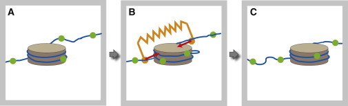
Example of a vector event. (A) The figure shows two steps of the translocation of one nucleosome (shown as a disk) along DNA. The dots (in green) along the DNA are position markers as a guide to the eye. In the first step (B), a chromatin remodeling enzyme binds to the nucleosome and applies equal but opposite forces on the DNA on opposite sides of the nucleosome. The enzyme is not shown, but its action is indicated by the spring (in orange). It leads to an excess of DNA wound around the nucleosome, which promotes formation of DNA loops that can diffuse along the nucleosome. In the second step (C), the enzyme detaches, and the extra DNA is released by the nucleosome, resulting in nucleosome translocation. (Gray frame) Limited field of view. For other illustrations of the production of force dipoles in chromatin, see Fig. 2 in Narlikar et al. (25) or Fig. 2 in Racki and Narlikar (3). Many other types of events in the nucleus are associated with generation of localized force dipoles including—but not limited to—the action of RNA polymerases, helicases, topoisomerases, etc. To see this figure in color, go online.

In Section S4 in the Supporting Material, we show that such a distribution of vector events can be included in our formalism as a contribution to the divergence of the active part of the stress tensor,

$$\overrightarrow{\nabla }\cdot {\overleftrightarrow{\sigma }}^{\left(\text{ac}\right)}\left(\overrightarrow{r},t\right)=fa\sum _{k=1}^{{\mathcal{M}}_v}{\hat{n}}_k\left({\hat{n}}_k\cdot \overrightarrow{\nabla }\right)\delta \left(\overrightarrow{r}-{\overrightarrow{R}}_k\right)g\left(t-t_k\right),$$ (19)

with $\mathcal{M}$_v the number of vector events in the time interval Δt. Each force dipole is composed of a pair of collinear opposing forces $f{\hat{n}}_k$ and $-f{\hat{n}}_k$ separated by a microscopic distance a. Here ${\hat{n}}_k$ is a unit vector along the force direction. For the case of nucleosome rearrangement events, a would have the typical size of a spacer length between nucleosomes.

Single vector event

A single active vector event at the origin at time t = 0 induces a transverse velocity flow field given by

$${\overrightarrow{v}}_{\perp }\left(\overrightarrow{q},\omega \right)=ifag\left(\omega \right)\frac{\overleftrightarrow{P}\left(\overrightarrow{q}\right)\cdot \hat{n}\left(\hat{n}\cdot \overrightarrow{q}\right)}{q^{2}E\left(q,\omega \right)}.$$ (20)

Here, $P_{ij}\left(\overrightarrow{q}\right)={\delta }_{ij}-{\hat{q}}_i{\hat{q}}_j$ is the transverse projection operator defined with $\hat{q}=\overrightarrow{q}/q$ and ${\hat{q}}_i=q_i/q$. The equation for the transverse flow field is obtained by applying this projection operator to Eqs. 1 and 2. The transverse polymer and solvent flow velocities are the same in this case (and hereon indicated as the flow field, itself). The inverse Fourier transform can be viewed as the Green’s function for vector events. For the special case of a Newtonian fluid, the flow field can be obtained explicitly, as discussed in Section S5 in the Supporting Material. The pattern of flow lines is that of extensional flow oriented along the force direction.

Distributed vector events

The flow field produced by a distribution of vector events is obtained by the superposition of the flow fields of individual sources. The activity function for a distribution of vector events is the linear superposition of individual events of the form of Eq. 20:

$$\overrightarrow{\beta }\left(\overrightarrow{q},\omega \right)=ifag\left(\omega \right)\sum _{k=1}^{{\mathcal{M}}_v}\overleftrightarrow{P}\left(\overrightarrow{q}\right)\cdot {\hat{n}}_k\left({\hat{n}}_k\cdot \hat{q}\right)e^{i\left(\overrightarrow{q}\cdot {\overrightarrow{R}}_k+\omega t_k\right)}.$$ (21)

The associated flow field can be obtained by a simple linear response relation

$${\overrightarrow{v}}_{\perp }\left(\overrightarrow{q},\omega \right)=\frac{1}{qE\left(q,\omega \right)}\overrightarrow{\beta }\left(\overrightarrow{q},\omega \right).$$ (22)

If, as for the scalar case, the ensemble-averaged flow field is very small, then the PSD of the velocity fluctuations is

$${\left({\overrightarrow{v}}_{\perp }^2\right)}_{\overrightarrow{q},\omega }={\left|\frac{1}{qE\left(q,\omega \right)}\right|}^2{\left({\overrightarrow{\beta }}^2\right)}_{\overrightarrow{q},\omega },$$ (23)

where the PSD for vector sources, ${\left({\overrightarrow{\beta }}^2\right)}_{\overrightarrow{q},\omega }$, is defined as in Eq. 13 for the scalar PSD.

To compare this expression with the PSD for transverse thermal equilibrium fluctuations, we use again the fluctuation-dissipation theorem:

$${\left({\overrightarrow{v}}_{\perp }^2\right)}_{\overrightarrow{q},\omega }\simeq \frac{4k_{\text{B}}T}{q^2}\text{Re}\left[\frac{1}{E\left(q,\omega \right)}\right].$$ (24)

This should be compared with the full Landau-Lifshitz expression for thermal hydrodynamic fluctuations in a Newtonian fluid (see, e.g., Lifshitz and Pitaevskii (26)),

$${\left({\overrightarrow{v}}_{\perp }^2\right)}_{\overrightarrow{q},\omega }=k_{\text{B}}T\frac{4\eta q^2}{{\left(\omega \rho \right)}^2+{\eta }^2{q}^4},$$ (25)

with ρ the mass density. For frequencies small compared to ηq²/ρ, the two expressions agree if one sets E = η.

Comparing the spectrum of active fluctuations with that of transverse equilibrium thermal fluctuations, one sees that—unlike the scalar case—active vectorial events are not reduced by a factor q² as compared to the equilibrium fluctuation spectrum. If active events have a long lifetime, then the active spectrum carries again an extra factor 1/ω². In that case, active vector events should dominate at low frequencies.

Nematic order parameter

Ensemble averaging for vectorial events can be discussed conveniently by introducing a nematic order parameter field. A force dipole source, Eq. 19, (locally) breaks rotational symmetry at the site of the force dipole event while maintaining inversion symmetry $\hat{n}\leftrightarrow -\hat{n}$ as reflected by Eq. 21. If the orientations of different force dipoles across the chromatin are correlated, then rotational symmetry could be broken on larger length scales. To examine the development of nematic order, we define the density ${\rho }_v\left(\overrightarrow{r},t\right)$ of vector events and the nematic order parameter as

$${\rho }_v\left(\overrightarrow{r},t\right)=\sum _k\delta \left(\overrightarrow{r}-{\overrightarrow{R}}_k\right)\delta \left(t-t_k\right),$$ (26a)

$$Q_{ij}\left(\overrightarrow{r},t\right)=\sum _k\delta \left(\overrightarrow{r}-{\overrightarrow{R}}_k\right)\delta \left(t-t_k\right)\left[{\hat{n}}_i^{\left(k\right)}{\hat{n}}_j^{\left(k\right)}-\frac{1}{3}{\delta }_{ij}\right].$$ (26b)

A similar formulation, in terms of fields instead of individual events, can be found in MacKintosh and Levine (27). In terms of the force dipole distribution, a chromatin solution would be a uniaxial or biaxial nematic if the spatial and temporal average 〈Q_ij〉 of $Q_{ij}\left(\overrightarrow{r},t\right)$ would be nonzero. In terms of the event density and the nematic order parameter field, Eq. 19 then reads as

$$\overrightarrow{\nabla }\cdot {\overleftrightarrow{\sigma }}^{\left(\text{ac}\right)}\left(\overrightarrow{r},t\right)=fa\int d^3{\overrightarrow{r}}^{\prime }d{t}^{\prime }g\left(t-t^{\prime }\right)\times \left[\overleftrightarrow{Q}\left({\overrightarrow{r}}^{\prime },t^{\prime }\right)+\frac{1}{3}\overleftrightarrow{I}\rho \left({\overrightarrow{r}}^{\prime },t^{\prime }\right)\right]\cdot \overrightarrow{\nabla }\delta \left(\overrightarrow{r}-{\overrightarrow{r}}^{\prime }\right).$$ (27)

An ensemble-averaged activity function for vectorial events $\langle \overrightarrow{\beta }\left(\overrightarrow{q},\omega \right)\rangle$ can be defined in analogy to the ensemble-averaged activity function $\langle \alpha \left(\overrightarrow{q},\omega \right)\rangle$ for scalar activity. In terms of the nematic order parameter:

$$\langle \overrightarrow{\beta }\left(\overrightarrow{q},\omega \right)\rangle =ifag\left(\omega \right)\overleftrightarrow{P}\left(\overrightarrow{q}\right)\cdot \langle \overleftrightarrow{Q}\left(\overrightarrow{q},\omega \right)\rangle \cdot \hat{q}.$$ (28)

The nucleus could have a broken rotational symmetry of the nematic type either because the orientations of the different force dipoles are correlated due to the intrinsic structural organization of the nucleus (which may or may not be related to the liquid-crystalline ordering possible in the suspensions of nucleosome particles (28)). Another, and even more interesting, possibility is that the symmetry-breaking is dynamic. The hydrodynamic backflow of active force dipoles produces the aligning torques on neighboring dipoles. Spontaneous nematic symmetry-breaking of this type has been invoked as a possible mechanism for the convective flows observed in oocytes (29).

If the fluctuations in chromatin are sufficiently strong that the ensemble-averaged nematic order parameter is zero, then—as in the scalar case—the PSD for nematic fluctuations can be expressed in the form of a two-point correlation function. In terms of the nematic order parameter field:

$${\left({\overrightarrow{\beta }}^2\right)}_{\overrightarrow{q},\omega }=f^2{a}^2|g\left(\omega \right){|}^2\times \frac{\langle \hat{q}\cdot {\overleftrightarrow{Q}}^{\text{∗}}\left(\overrightarrow{q},\omega \right)\cdot \overleftrightarrow{P}\left(\overrightarrow{q}\right)\cdot \overleftrightarrow{Q}\left(\overrightarrow{q},\omega \right)\cdot \hat{q}\rangle }{\Delta V\Delta T}.$$ (29)

Similar to the formula in Eq. 14, the PSD of vector events simplifies if the directions of the force dipoles are statistically independent of each other and of the event positions. In that case, only the k = k′ terms survive in the double summation over event pairs implicit in the formula of Eq. 29, which results in

$${\left({\overrightarrow{\beta }}^2\right)}_{\overrightarrow{q},\omega }={\rho }_v{f}^2{a}^2{\left|g\left(\omega \right)\right|}^2\langle {\left(\hat{q}\cdot \hat{n}\right)}^2-{\left(\hat{q}\cdot \hat{n}\right)}^4\rangle ,$$ (30)

where ρ_v is the average of ${\rho }_v\left(\overrightarrow{r},t\right)$. If the force dipoles are distributed isotropically, then

$$\langle {\left(\hat{q}\cdot \hat{n}\right)}^2-{\left(\hat{q}\cdot \hat{n}\right)}^4\rangle =2/15\text{.}$$

Results and Comparison with Experiment

This section provides a preliminary comparison of the theoretical framework of the previous sections with the observational study of collective dynamics in chromatin that motivated our work. The observational study applied displacement correlation spectroscopy (DCS), which is based on time-resolved image correlation analysis as a means for the measurement of the velocity fluctuation spectra (19). DCS uses algorithms of particle image velocimetry to measure direction and magnitude of local movements simultaneously across the entire nucleus and over the entire duration of the experiment (19). Fluorescently-labeled histones are used to visualize chromatin movement. A camera records subsequent exposures to pulses of laser light. The frames are split into a large number of interrogation areas, or windows. For each interrogation window a local displacement vector between two time points, separated by time interval Δt, is obtained by cross-correlation between pairs of images; all experimentally accessible values of Δt were sampled. If the displacement over a time interval Δt is measured, then the mean velocity

$$\left[\overrightarrow{r}\left(t+\Delta t\right)-\overrightarrow{r}\left(t\right)\right]/\Delta t$$

can be obtained. The spatial Fourier transform $\overrightarrow{F}\left(\overrightarrow{q},\Delta t\right)$ of the mean flow velocity is given by

$$\overrightarrow{F}\left(\overrightarrow{q},\Delta t\right)=\sum _j^N\frac{\overrightarrow{r_j}\left(t+\Delta t\right)-\overrightarrow{r_j}\left(t\right)}{\Delta t}{e}^{i\overrightarrow{q}\cdot {\overrightarrow{r}}_j\left(t\right)},$$ (31)

with N the number of tracer particles. The flow spectral density (FSD) S(q,Δt) is defined as

$$\langle {\left|\overrightarrow{F}\left(q,\Delta t\right)\right|}^2\rangle /N.$$

In Section S6 in the Supporting Material we show that this measured FSD is related to the computed velocity PSD by,

$$S\left(q,\Delta t\right)\simeq c\int \frac{1-\text{cos}\omega \Delta t}{{\left(\omega \Delta t\right)}^2}{\left({\overrightarrow{v}}^2\right)}_{\overrightarrow{q},\omega }\frac{d\omega }{\pi },$$ (32)

with c = N/ΔV the tracer concentration.

In the study, the time-dependent displacements of labeled chromatin sites,

$${\overrightarrow{r}}_i\left(t+\Delta t\right)-{\overrightarrow{r}}_i\left(t\right),$$

were measured for interphase HeLa cells both with and without ATP consumption (19). From these data, we calculated the FSD using the method described above. Fig. 3 shows the measured FSD as a function of the wavenumber q for different values of Δt.

Figure 3.

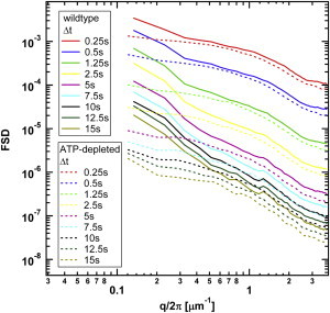
Flow spectral densities of the chromatin of wild-type and ATP-depleted nuclei of interphase HeLa cells as a function of the wavenumber q for several values of the fixed measurement time interval Δt. To see this figure in color, go online.

We fitted the data to the form

$$S\left(q,\Delta t\right)=A\left(q\right)/\Delta t^2+B\left(q\right)/\Delta t.$$ (33)

The motivation for this fitting function was twofold. In the limit that the wavenumber q is larger than the inverse of the mean separation between the tracer particles, the FSD should be proportional to 1/Δt² for localized tracer particles and proportional to 1/Δt for diffusing tracer particles (see Section S6 in the Supporting Material). We will discuss below that this is also a natural fitting form for general q when a simple model for the E(q,ω) value of chromatin is adopted.

The result of a fit to the passive data (ATP-depleted nuclei) is shown in Fig. 4. The best fit is A(q) ∝ 1/q^1.6 whereas B(q) is statistically very close to zero for the q/2π value in excess of an inverse micron. The inset of Fig. 4 shows the FSD multiplied by Δt² as a function of Δt for fixed q. Because B(q) is statistically almost zero, this should be practically a horizontal straight line for the fitting procedure to be meaningful. This appears to be the case. Recall that in terms of tracer dynamics, a Δt² dependence would indicate localization.

Figure 4.

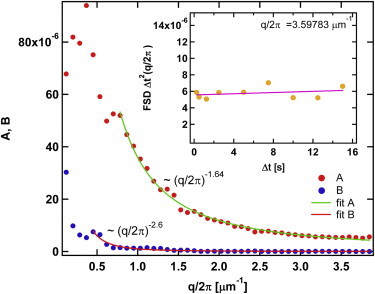
Fit coefficients A(q) and B(q) of the fitting form of Eq. 33 for the case of ATP-depleted cells. B(q) is practically zero for q/2π greater than an inverse micron; that means that the FSD at constant q should be proportional to 1/Δt². (Inset) Passive FSD multiplied by Δt² for fixed q as a function of Δt; linear regression (pink line), very nearly horizontal. To see this figure in color, go online.

The next step should be a comparison between the measured FSD and the FSD computed for a generalized complex shear viscosity E(q,ω) obtained either from a microrheological study or a microscopic theory of chromatin rheology. As neither is available at this point, we will assume

$$E\left(\omega \right)=\frac{\eta }{1-i\omega \tau }$$

independent of wavenumber as a simple illustrative example. This form is the generalized viscosity of the Maxwell fluid (MF). Based on the Tseng et al. (15), Celedon et al. (17), Pajerowski et al. (18), and Dahl et al. (30), our best estimates are for τ to be in the range of a few seconds and for η/τ to be in the range of 1.5–200 Pa. In Section S7 in the Supporting Material, it is shown that the FSD of a passive MF is the sum of a longitudinal velocity term (approximately) proportional to 1/(q²Δt²) for Δt large compared to the inverse of the relaxation rates of the MF, and a transverse velocity term proportional to 1/(q²Δt). In terms of a comparison with the MF, our results would seem to rule out transverse velocity fluctuations as the source of the observed equilibrium FSD because of the Δt dependence. However, the q dependence of the FSD deviates somewhat from the MF 1/q² dependence; the heterogeneity of chromatin could be a contributing factor in this regard (because the local chromatin concentration varies throughout the nucleus in a living cell significantly), or it could indicate that a q dependence must be included in the MF expression for the generalized viscosity. It should be noted that the viscosity of the nucleoplasm is known to be time-dependent (31) but this takes place over timescales that are much longer than the duration of the experiment (∼25 s).

At the next stage, we repeated the analysis for the case of wild-type HeLa cells, which are ATP-active. For values of q/2π larger than an inverse micron, the passive (ATP-depleted) and active (wild-type, ATP-active) spectra appear to be quite similar, apart from the roughly doubled overall intensity (see Fig. 3). The simplest interpretation is that in this high q regime the FSD still is dominated by thermal fluctuations but that ATP activity has reduced the osmotic modulus by a factor of approximately one-half. In principle, it is also possible that large q active fluctuations have the same form as thermal fluctuations, but with an effective noise-temperature that is twice the actual temperature.

For q/2π less than an inverse micron, the active and passive spectra are different: the FSD of the active system increases rapidly, as compared to the passive data (Fig. 3). Equation 33 still can be used as a fitting form. This is demonstrated in the inset in Fig. 5, which shows a plot of the FSD multiplied by (Δt)² for a fixed q roughly corresponding to the crossover between large and small q regimes (where passive and active data are very similar and very different, respectively). It is seen that the FSD multiplied by Δt² is approximately linear in Δt (the linear regression fit is shown as a solid straight line). Having justified the fitting from Eq. 33, we analyzed the coefficients A(q) and B(q) obtained from the fitting procedure. The data for large q regime are shown in Fig. 5. Just as for the passive case, B(q) is very small for q/2π that is larger than an inverse micron. On the other hand, in the low q range, B(q) grows so rapidly that it has to be plotted on a different vertical scale (see Fig. S2 in the Supporting Material).

Figure 5.

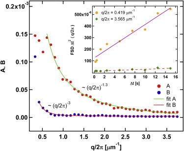
Fit coefficients A(q) and B(q) of the fitting form of Eq. 33 for the case of ATP-consuming cells. (Inset) FSD multiplied by Δt² of wild-type (ATP-consuming) cells for two particular fixed values of q as a function of Δt; (solid and dashed lines) linear regression fits. To see this figure in color, go online.

The inset in Fig. 5 that demonstrates linear dependence would be consistent with a FSD that is inversely proportional to 1/Δt. In turn, this would be consistent with diffusive tracer dynamics. In terms of a comparison between the FSD of active cells and that of MF rheology, we show in Section S7 in the Supporting Material that the contribution to the FSD coming from active transverse velocity fluctuations is proportional to 1/q²Δt, just as it was for thermal fluctuations. The contribution coming from active longitudinal fluctuations is either independent of q or goes to zero in the small q limit, depending on whether Δt is small or large compared to the duration of the active events. In either case, the longitudinal FSD would be proportional to 1/Δt, which is not consistent with the observed Δt dependence. The interpretation of these results in terms of the MF would be that, for ATP-consuming cells, transverse active fluctuations dominate in the small q limit whereas longitudinal thermal fluctuations dominate for larger q.

Conclusions

To summarize, we have presented a framework for the analysis of large-scale studies of chromatin dynamics using particle-tracking methods. It is based on the assumption that the response of chromatin to equilibrium thermal fluctuations, active concentration fluctuations, and active force dipoles can be described by linearized hydrodynamics. The proposed method was illustrated by applying it to the results of a recent DCS study of global chromatin dynamics. If the results are interpreted in terms of single-particle dynamics, they indicate a crossover from localized dynamics in ATP-depleted cells to diffusive dynamics in ATP-active cells. This is consistent with some of the single-particle tracking studies (e.g., Levi et al. (10)). In terms of an interpretation based on the MF, thermal fluctuations of ATP-depleted cells are dominated by concentration fluctuations. For ATP-active cells, small wavelength fluctuations (i.e., wavenumbers larger than a few inverse microns) are still dominated by concentration fluctuations. The increase of the intensity of the fluctuations could be due to a simple reduction of the osmotic modulus in the presence of ATP hydrolysis. Longer wavelength fluctuations appear to be associated with transverse velocity fluctuations generated by force-dipole activity.

It should be pointed out that boundary effects associated with the nuclear membrane are likely to play an important role for fluctuations with a wavelength comparable to the size of the nucleus. Large-scale concentration fluctuations should be suppressed by a rigid boundary. Indeed, on the timescales relevant for the experiments discussed above (≲10 s), the nuclear membrane is effectively rigid (19) (see also Hinde et al. (13) and Talwar et al. (32)). Coupling between nuclear envelope breathing and internal chromatin dynamics in embryonic stem cells on timescales upwards of ∼100 s was examined in Talwar et al. (32) and would have to be included for the theory to be extended into this frequency range. Based on the results of a recent study of the convective dynamics driven by active force dipoles inside a sphere as a model for cytoplasmic streaming (33), active transverse flow fluctuations with q in the range of the inverse of the nucleus are not expected to be suppressed, although they may be scattered by the concentration inhomogeneities that characterize chromatin. One interesting possibility is that coupling of the dipoles through the medium leads to a form of nematic order.

Another open question concerns the actual form of the generalized complex viscosity E(q,ω). Studies of the local topology of chromatin have concluded that it has a fractal structure, specifically that of a crumpled globule (34–36). Theoretical studies of the rheological properties of polymer melts (in which polymers have the fractal geometry of Gaussian chains) indicate that even in this simple case E(q,ω) does not have the MF form (37). Understanding the connection between the fractal structure of chromatin and its rheological properties poses an interesting theoretical challenge.

Finally, we would like to put our work in the broader context of complex materials and systems. To the best of our knowledge, the possibility of active scalar events has not been considered in the literature. However, sequences of force-dipole events have been discussed in relation to punctuated stress relaxation phenomena in amorphous media, such as glasses or foams (see, e.g., Chattoraj et al. (37)). An interesting possibility would be to apply the PSD/FSD measurement method discussed here to other active systems, such as a suspension of actively swimming microorganisms (38–40).

References

- 1.Alberts B., Johnson A., Walter P. Garland Science; New York: 2008. Molecular Biology of the Cell. [Google Scholar]
- 2.Cremer T., Cremer C. Chromosome territories, nuclear architecture and gene regulation in mammalian cells. Nat. Rev. Genet. 2001;2:292–301. doi: 10.1038/35066075. [DOI] [PubMed] [Google Scholar]
- 3.Racki L.R., Narlikar G.J. ATP-dependent chromatin remodeling enzymes: two heads are not better, just different. Curr. Opin. Genet. Dev. 2008;18:137–144. doi: 10.1016/j.gde.2008.01.007. [DOI] [PMC free article] [PubMed] [Google Scholar]
- 4.Hansen J.C. Human mitotic chromosome structure: what happened to the 30-nm fiber? EMBO J. 2012;31:1621–1623. doi: 10.1038/emboj.2012.66. [DOI] [PMC free article] [PubMed] [Google Scholar]
- 5.Dekker J., van Steensel B. Chapt. 7: The spatial architecture of chromosomes. In: Walhout M., Vidal M., Dekker J., editors. Handbook of Systems Biology: Concepts and Insights. Elsevier; New York: 2013. pp. 137–151. [Google Scholar]
- 6.Marshall W.F., Straight A., Sedat J.W. Interphase chromosomes undergo constrained diffusional motion in living cells. Curr. Biol. 1997;7:930–939. doi: 10.1016/s0960-9822(06)00412-x. [DOI] [PubMed] [Google Scholar]
- 7.Bornfleth H., Edelmann P., Cremer C. Quantitative motion analysis of subchromosomal foci in living cells using four-dimensional microscopy. Biophys. J. 1999;77:2871–2886. doi: 10.1016/S0006-3495(99)77119-5. [DOI] [PMC free article] [PubMed] [Google Scholar]
- 8.Heun P., Laroche T., Gasser S.M. Chromosome dynamics in the yeast interphase nucleus. Science. 2001;294:2181–2186. doi: 10.1126/science.1065366. [DOI] [PubMed] [Google Scholar]
- 9.Bronstein I., Israel Y., Garini Y. Transient anomalous diffusion of telomeres in the nucleus of mammalian cells. Phys. Rev. Lett. 2009;103:018102. doi: 10.1103/PhysRevLett.103.018102. [DOI] [PubMed] [Google Scholar]
- 10.Levi V., Ruan Q., Gratton E. Chromatin dynamics in interphase cells revealed by tracking in a two-photon excitation microscope. Biophys. J. 2005;89:4275–4285. doi: 10.1529/biophysj.105.066670. [DOI] [PMC free article] [PubMed] [Google Scholar]
- 11.Hameed F.M., Rao M., Shivashankar G.V. Dynamics of passive and active particles in the cell nucleus. PLoS ONE. 2012;7:e45843. doi: 10.1371/journal.pone.0045843. [DOI] [PMC free article] [PubMed] [Google Scholar]
- 12.Weber S.C., Spakowitz A.J., Theriot J.A. Nonthermal ATP-dependent fluctuations contribute to the in vivo motion of chromosomal loci. Proc. Natl. Acad. Sci. USA. 2012;109:7338–7343. doi: 10.1073/pnas.1119505109. [DOI] [PMC free article] [PubMed] [Google Scholar]
- 13.Hinde E., Cardarelli F., Gratton E. Tracking the mechanical dynamics of human embryonic stem cell chromatin. Epigen. Chromatin. 2012;5:20. doi: 10.1186/1756-8935-5-20. [DOI] [PMC free article] [PubMed] [Google Scholar]
- 14.Meshorer E., Yellajoshula D., Misteli T. Hyperdynamic plasticity of chromatin proteins in pluripotent embryonic stem cells. Dev. Cell. 2006;10:105–116. doi: 10.1016/j.devcel.2005.10.017. [DOI] [PMC free article] [PubMed] [Google Scholar]
- 15.Tseng Y., Lee J.S.H., Wirtz D. Micro-organization and visco-elasticity of the interphase nucleus revealed by particle nanotracking. J. Cell Sci. 2004;117:2159–2167. doi: 10.1242/jcs.01073. [DOI] [PubMed] [Google Scholar]
- 16.de Vries A.H.B., Krenn B.E., Kanger J.S. Direct observation of nanomechanical properties of chromatin in living cells. Nano Lett. 2007;7:1424–1427. doi: 10.1021/nl070603+. [DOI] [PubMed] [Google Scholar]
- 17.Celedon A., Hale C.M., Wirtz D. Magnetic manipulation of nanorods in the nucleus of living cells. Biophys. J. 2011;101:1880–1886. doi: 10.1016/j.bpj.2011.09.008. [DOI] [PMC free article] [PubMed] [Google Scholar]
- 18.Pajerowski J.D., Dahl K.N., Discher D.E. Physical plasticity of the nucleus in stem cell differentiation. Proc. Natl. Acad. Sci. USA. 2007;104:15619–15624. doi: 10.1073/pnas.0702576104. [DOI] [PMC free article] [PubMed] [Google Scholar]
- 19.Zidovska A., Weitz D.A., Mitchison T.J. Micron-scale coherence in interphase chromatin dynamics. Proc. Natl. Acad. Sci. USA. 2013;110:15555–15560. doi: 10.1073/pnas.1220313110. [DOI] [PMC free article] [PubMed] [Google Scholar]
- 20.Marchetti M., Joanny J., Simha R.A. Hydrodynamics of soft active matter. Rev. Mod. Phys. 2013;85:1143–1189. [Google Scholar]
- 21.Doi M., Onuki A. Dynamic coupling between stress and composition in polymer solutions and blends. J. Phys. II (France) 1992;2:1631–1656. [Google Scholar]
- 22.Landau L.D., Lifshitz E.M. Course of Theoretical Physics, Vol. 5. 3rd Ed. Butterworth-Heinemann; Oxford, UK: 1980. Statistical physics, part 1. [Google Scholar]
- 23.Doi M. Oxford University Press; Oxford, UK: 2013. Soft Matter Physics. [Google Scholar]
- 24.Milner S.T. Dynamical theory of concentration fluctuations in polymer solutions under shear. Phys. Rev. E Stat. Phys. Plasmas Fluids Relat. Interdiscip. Topics. 1993;48:3674–3691. doi: 10.1103/physreve.48.3674. [DOI] [PubMed] [Google Scholar]
- 25.Narlikar G.J., Sundaramoorthy R., Owen-Hughes T. Mechanisms and functions of ATP-dependent chromatin-remodeling enzymes. Cell. 2013;154:490–503. doi: 10.1016/j.cell.2013.07.011. [DOI] [PMC free article] [PubMed] [Google Scholar]
- 26.Lifshitz E.M., Pitaevskii L.P. Vol. 9. Butterworth-Heinemann; Oxford, UK: 2002. Statistical physics, part 2: theory of the condensed state. (Course of Theoretical Physics). [Google Scholar]
- 27.MacKintosh F.C., Levine A.J. Nonequilibrium mechanics and dynamics of motor-activated gels. Phys. Rev. Lett. 2008;100:018104. doi: 10.1103/PhysRevLett.100.018104. [DOI] [PubMed] [Google Scholar]
- 28.Mangenot S., Leforestier A., Livolant F. Phase diagram of nucleosome core particles. J. Mol. Biol. 2003;333:907–916. doi: 10.1016/j.jmb.2003.09.015. [DOI] [PubMed] [Google Scholar]
- 29.Ganguly S., Williams L.S., Goldstein R.E. Cytoplasmic streaming in Drosophila oocytes varies with kinesin activity and correlates with the microtubule cytoskeleton architecture. Proc. Natl. Acad. Sci. USA. 2012;109:15109–15114. doi: 10.1073/pnas.1203575109. [DOI] [PMC free article] [PubMed] [Google Scholar]
- 30.Dahl K.N., Engler A.J., Discher D.E. Power-law rheology of isolated nuclei with deformation mapping of nuclear substructures. Biophys. J. 2005;89:2855–2864. doi: 10.1529/biophysj.105.062554. [DOI] [PMC free article] [PubMed] [Google Scholar]
- 31.Liang L., Wang X., Chen W.R. Noninvasive determination of cell nucleoplasmic viscosity by fluorescence correlation spectroscopy. J. Biomed. Opt. 2009;14:024013. doi: 10.1117/1.3088141. [DOI] [PubMed] [Google Scholar]
- 32.Talwar S., Kumar A., Shivashankar G.V. Correlated spatio-temporal fluctuations in chromatin compaction states characterize stem cells. Biophys. J. 2013;104:553–564. doi: 10.1016/j.bpj.2012.12.033. [DOI] [PMC free article] [PubMed] [Google Scholar]
- 33.Woodhouse F.G., Goldstein R.E. Spontaneous circulation of confined active suspensions. Phys. Rev. Lett. 2012;109:168105. doi: 10.1103/PhysRevLett.109.168105. [DOI] [PubMed] [Google Scholar]
- 34.Grosberg A.Y., Rabin Y., Neer A. Crumpled globule model of three-dimensional structure of DNA. Europhys. Lett. 1993;23:373–378. [Google Scholar]
- 35.Lieberman-Aiden E., van Berkum N.L., Dekker J. Comprehensive mapping of long-range interactions reveals folding principles of the human genome. Science. 2009;326:289–293. doi: 10.1126/science.1181369. [DOI] [PMC free article] [PubMed] [Google Scholar]
- 36.Bancaud A., Lavelle C., Ellenberg J. A fractal model for nuclear organization: current evidence and biological implications. Nucleic Acids Res. 2012;40:8783–8792. doi: 10.1093/nar/gks586. [DOI] [PMC free article] [PubMed] [Google Scholar]
- 37.Chattoraj J., Caroli C., Lemaître A. Robustness of avalanche dynamics in sheared amorphous solids as probed by transverse diffusion. Phys. Rev. E Stat. Nonlin. Soft Matter Phys. 2011;84:011501. doi: 10.1103/PhysRevE.84.011501. [DOI] [PubMed] [Google Scholar]
- 38.Hatwalne Y., Ramaswamy S., Simha R.A. Rheology of active-particle suspensions. Phys. Rev. Lett. 2004;92:118101. doi: 10.1103/PhysRevLett.92.118101. [DOI] [PubMed] [Google Scholar]
- 39.Chen D.T.N., Lau A.W.C., Yodh A.G. Fluctuations and rheology in active bacterial suspensions. Phys. Rev. Lett. 2007;99:148302. doi: 10.1103/PhysRevLett.99.148302. [DOI] [PubMed] [Google Scholar]
- 40.Lau A.W.C., Lubensky T.C. Fluctuating hydrodynamics and microrheology of a dilute suspension of swimming bacteria. Phys. Rev. E Stat. Nonlin. Soft Matter Phys. 2009;80:011917. doi: 10.1103/PhysRevE.80.011917. [DOI] [PubMed] [Google Scholar]
Associated Data
This section collects any data citations, data availability statements, or supplementary materials included in this article.