Abstract
State-of-the-art fluoroscopic knee kinematic analysis methods require the patient-specific bone shapes segmented from CT or MRI. Substituting the patient-specific bone shapes with personalizable models, such as statistical shape models (SSM), could eliminate the CT/MRI acquisitions, and thereby decrease costs and radiation dose (when eliminating CT). SSM based kinematics, however, have not yet been evaluated on clinically relevant joint motion parameters.
Therefore, in this work the applicability of SSM-s for computing knee kinematics from biplane fluoroscopic sequences was explored. Kinematic precision with an edge based automated bone tracking method using SSM-s was evaluated on 6 cadaver and 10 in-vivo fluoroscopic sequences. The SSMs of the femur and the tibia-fibula were created using 61 training datasets. Kinematic precision was determined for medial-lateral tibial shift, anterior-posterior tibial drawer, joint distraction-contraction, flexion, tibial rotation and adduction. The relationship between kinematic precision and bone shape accuracy was also investigated.
The SSM based kinematics resulted in sub-millimeter (0.48–0.81 mm) and approximately one degree (0.69–0.99°) median precision on the cadaveric knees compared to bone-marker-based kinematics. The precision on the in-vivo datasets was comparable to the cadaveric sequences when evaluated with a semi-automatic reference method. These results are promising, though further work is necessary to reach the accuracy of CT-based kinematics. We also demonstrated that a better shape reconstruction accuracy does not automatically imply a better kinematic precision. This result suggests that the ability of accurately fitting the edges in the fluoroscopic sequences has a larger role in determining the kinematic precision than the overall 3D shape accuracy.
Keywords: Ttracking, SSM, Femur, Tibia, 2D/3D reconstruction
Introduction
Knee kinematics measurements are performed to describe normal joint function (Giphart et al., 2008; Li et al., 2005; Torry et al., 2010), to improve prosthesis designs (Kitagawa et al., 2010), and to characterize injury (Defrate et al., 2006; Dennis et al., 2005).
The most accurate method to assess joint kinematics is biplane fluoroscopy using metallic markers inserted in the bones to assess their pose through time (Tashman and Anderst, 2003). As marker insertion is invasive, this technique is not suitable in most cases. Skin marker-based kinematics on the other hand is prone to soft-tissue motion resulting in errors larger than 10 mm (Garling et al., 2007; Stagni et al., 2005). More accurate kinematics can be obtained with model-based tracking in fluoroscopy (Fregly et al., 2005; Kitagawa et al., 2010; Li et al., 2008; Muhit et al., 2010; Nakajima et al., 2007; Pickering et al., 2009; Scott and Barney Smith, 2006; Tsai et al., 2010; You et al., 2001). These methods align a 3D bone model, segmented from CT or MRI, with calibrated fluoroscopic sequences. Alignment is achieved by minimizing either an image intensity distance through calculation of digitally reconstructed radiographs (DRR) (Anderst et al., 2009; Bey et al., 2008; Dennis et al., 2005; Mahfouz et al., 2003; Muhit et al., 2010; Nakajima et al., 2007; Pickering et al., 2009; Scott and Barney Smith, 2006; You et al., 2001), or an image edge to bone model silhouette distance (Defrate et al., 2006; Fregly et al., 2005; Gollmer et al., 2007; Hanson et al., 2006; Hirokawa et al., 2008; Kitagawa et al., 2010; Li et al., 2008; Tersi et al., 2012; Torry et al., 2011; Tsai et al., 2010). Kinematic analysis not requiring the subject-specific 3D model would, however, be preferred, as it would lower analysis costs and eliminate the prior 3D acquisition resulting in lower radiation dose in the case of CT.
Statistical shape models (SSM) could replace subject-specific shapes, as they are able to generate previously unseen shapes resembling the population they were built on. SSM-s have been applied for reconstruction of bone shapes from single time-point biplane X-ray images (Baka et al., 2011; Gamage et al., 2009; Whitmarsh et al., 2011; Zheng et al., 2008; Zhu and Li, 2011). They have recently also been proposed for kinematic analysis differentiating between healthy and pathologic wrists (Chen et al., 2011), and assessing femur kinematics from in-vivo drop-landing sequences (Baka et al., 2012).
While first results with SSM based tracking were encouraging, the lack of evaluations of clinically relevant joint motion parameters makes the accuracy of SSM based joint kinematics yet unknown. Also, several studies indicated, that the accuracy of the 3D bone surface may influence the kinematic accuracy (Moewis et al., 2012; Moro-oka et al., 2007). The aim of this study was, therefore, to explore the applicability of SSM-s for calculating knee kinematics from biplane fluoroscopy. The following research questions were posed:
Does the 3D shape reconstruction accuracy influence the kinematic tracking precision?
What kinematic tracking precision can we achieve with the SSM using an automated edge based approach?
We performed experiments on high-speed biplane fluoroscopic sequences analyzing the drop-landing motion of 6 cadaveric and 10 in-vivo knees.
Data
Kinematic data
The in-vivo dataset consisted of 10 drop-land sequences acquired with a high-speed (500 frames/sec), high resolution (1024×1024 pixels), custom built biplane fluoroscopic setup. The sequences were part of earlier studies (Torry et al., 2011, 2010), where the acquisition setup was described in detail. Briefly, subjects were asked to perform a drop-landing from a 40 cm high box, and land on their dominant leg in the field-of-view (FOV) of the biplane fluoroscopic camera system. The average sequence length was 74 frames. All subjects were also scanned by CT to attain the subject-specific knee shape.
The cadaver dataset consisted of 6 intact cadaveric knees, which were dropped in the FOV of the bi-plane fluoroscopic system to simulate the drop-landing motion. The sequences were part of an earlier study (Giphart et al., 2012), which contains more detail on the experimental setup. The bones were implanted with tantalum beads to enable marker-based kinematic analysis. All cadaveric knees were also scanned by CT.
Training set of the SSM
The training set of the SSM of the femur and the combined tibia-fibula consisted of 62 knee CT images, from which 10 were subjects from the in-vivo kinematic dataset, 47 were subjects scanned for other medical reasons than arthritis, and 5 were cadavers from the kinematic dataset. The population contained both sexes with a wide age range (subjects were 21-66 years old, the cadavers' age was unknown). The CT images were acquired on different scanners with in-plane voxel sizes between 0.6-0.78 mm, and slice thickness between 0.5-0.8 mm.
Method
Figure 1 depicts the diagram of a general feature-based knee kinematics method. First, the features (edges) in the fluoroscopic frames are extracted. Second, the femoral and tibial surface models are aligned in 3D space to best match the extracted features. Finally, the pose estimates of the femur and tibia over time are converted into knee kinematics by expressing the recovered motion in the anatomical coordinate-system of the knee.
Figure 1.
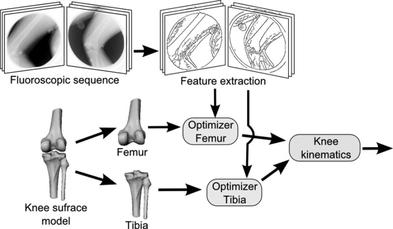
The diagram of a general feature based knee kinematics method. First, the features (edges) in the fluoroscopic images are extracted in every frame. Second, a surface model of the femur and the tibia is aligned in 3D space to best match the features in the fluoroscopic frames. Finally, the pose estimates of the femur and tibia through time are converted into knee kinematic measurements.
Variations of this framework include the traditional knee kinematics system using manual edge extraction and subject-specific knee surfaces, as well as the automated, 3D acquisition-free system using automatic edge extraction and SSM-generated knee shapes. We describe our implementation of the automated system below.
Statistical shape model
The CT images in the training set of the SSM (Cootes et al., 1992) were segmented using level-sets, and were converted to triangulated surfaces with the same number of corresponding landmark points (femur: 4250 points, tibia-fibula: 4778 points). Correspondence within the training set was achieved using B-spline registrations (Elastix (Klein et al., 2010)), by deforming every bone segmentation to match the bone with the smallest FOV, and subsequently propagating the surface points of this shortest bone back to every bone in the training set. Bones were then aligned by Procrustes analysis (translation, rotation, isotropic scaling), and principal component analysis (PCA) was employed to derive the statistical shape model consisting of the mean shape and its main modes of variations. New shapes can be generated with the model by varying the parameters along the modes. First and second modes of both models are shown in Figure 2. The models were created containing 95% of the variance resulting in 33 modes for the femur, and 32 modes for the tibia-fibula.
Figure 2.
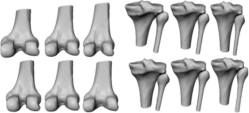
Illustration of the statistical shape models of the femur (left) and the tibia-fibula (right). The rows show the first and second mode of variation with parameters set to -3 std, 0, +3 std.
2D/3D bone reconstruction and tracking
Knee kinematics were recovered by optimizing the shape and the pose of the SSM through time to best fit the automatically extracted edges in the fluoroscopic frames. Edges were extracted with a Canny edge detector (Canny, 1986), employing hysteresis thresholding on the gradient magnitude. The optimization algorithm was derived from (Baka et al., 2012)1, consisting of three stages: 1) a crude alignment of the mean shape calculated frame-by-frame; 2) shape and pose estimation on a subset of frames2 (≤30). ;and 3) optimization of the pose of the reconstructed shape on all frames. The optimized error measure consisted of a shape prior and a data matching term. The Mahalanobis distance (Mahalanobis, 1936) between the reconstructed shape and the statistical shape distribution was used as shape prior. The data matching term was calculated as follows. For every projected contour point of the model a corresponding image edge pixel was selected. The contour points of the model were defined as points shared by two triangles from which one is facing, and the other is back-facing the X-ray source. The distance between projected contour point and edge pixel was determined from the 2D Euclidean distance and the angular distance between projected surface normal and image gradient. Distances of all contour points in all projection directions were then squared and summed to form the data matching term. The error function was minimized using a numeric optimizer. For details we refer to (Baka et al., 2012).
After calculating the pose parameters for the bones for every frame, we applied a weighted moving average smoother on the bone kinematics to reduce the effect of noise. We used a window size of 5, with weights [0.5, 1, 2,1, 0.5].
Experiments
We performed three sets of experiments to answer our research questions. In all experiments, the subject to be evaluated was left out from the training set of the SSM. All experiments were performed seven times with different initial positions drawn from a uniform random distribution (±5 mm and degrees3) around the reference standard pose in a chosen start frame, and were the same for all methods for fair comparison. The 7th frame with reference standard pose was chosen for the initialization as both femur and tibia were visible.
The following variants of the feature based knee kinematics framework shown in Figure 1 were evaluated in the experiments:
CTman: Optimizes the pose of the CT-derived (subject specific) knee surface using manual selection of edge segments in the fluoroscopic frames.
CTauto: Optimizes the pose of the CT-derived knee surface using automatic edge detection in the fluoroscopic frames.
Mauto: Optimizes the pose of the population mean knee surface using automatic edge detection.
Rauto: Optimizes the pose of the SSM representation of the CT-derived knee surface. The SSM is thus first fitted to the 3D CT segmentation (3D/3D fitting), and then kept constant for kinematic analysis. Automatic edge detection is applied.
SSMauto: Optimizes both shape and pose of the knee using an SSM (2D/3D fitting). Automatic edge detection is applied. This method is described in the Method Section.
The following experiments were performed:
Experiment 1: The performance of the automated edge selection was assessed by comparing the CTauto method with the semi-automatic CTman method. The evaluation was performed on the cadaver sequences enabling comparison with marker-based kinematics.
Experiment 2: To evaluate the influence of the shape accuracy on the tracking accuracy, shapes of different accuracy were matched on the cadaver dataset: the CT segmented bone surfaces (CTauto), their SSM representation (Rauto), the 2D/3D reconstructed shape (SSMauto), and the scaled population mean shapes (Mauto).
Experiment 3: This experiment was performed to evaluate kinematic parameters as well as shape reconstruction accuracy with the automated SSM based tracking (SSMauto), on both kinematic datasets.
Evaluation measures
Knee kinematics were calculated as proposed by (Grood and Suntay, 1983), quantifying medial-lateral (ML) tibial shift, anterior-posterior (AP) tibial drawer, joint distraction-contraction, flexion, tibial rotation and adduction. The femur and tibia coordinate-systems were specified according to (Miranda et al., 2010) in the CT-segmented bone shapes as illustrated in Figure 3. This coordinate-system was transferred to the SSM and the tantalium markers at a pre-defined frame in each sequence to enable comparison of kinematic parameters. The resulting kinematics were compared with CTman kinematics (reference standard), and with marker-based kinematics (gold standard) when available. Both were calculated in a subset (usually one quarter) of the frames using Model-based RSA (Model-based RSA, Medis-specials, Leiden, The Netherlands). The kinematic accuracy of a sequence was defined by a combination of bias and precision. Bias was calculated as the mean error of all frames, and precision as the standard deviation of the remaining error after removing the bias. Bias is dependent on the anatomic coordinate-systems used for kinematics calculation, and can range anywhere between 0 and several millimeters and degrees. Precision is less affected by coordinate-system differences, and is an indicator of the relative pose accuracy (e.g. change in joint distraction-contraction from before to after landing).
Figure 3.
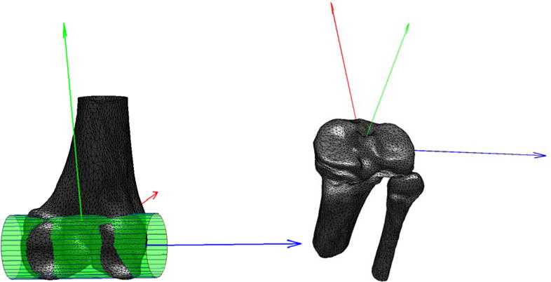
Femoral and tibial coordinate systems. A cylinder fitted to the posterior condyles determined the ML femoral axis (blue), whose mid-point served as origin. The AP axis (red) was defined perpendicular to the ML axis and the femoral shaft. The proximal-distal (PD) axis (green) was set orthogonal to the AP and ML directions. For the tibial coordinate-system, the tibial plateau was identified as the plane with the largest surface area orthogonal to the tibial shaft. The plateau's center of mass was used as origin, and its inertial axes as the ML (blue) and AP (red) axes.
Shape reconstruction accuracy was calculated as the root mean square (RMS) distance of all CT segmented bone surface points to the reconstructed surface. The reconstructed surface was aligned with the CT by a 3D/3D rigid registration prior to the accuracy measurement.
Results
Experiment 1 focused on validating the automated kinematic analysis by comparing it with the semi-automatic reference standard using the CT-derived bones. The resulting precision and bias are summarized in Figure 4. The median translation and rotation precision with CTman averaged over the three anatomical directions was 0.62 mm and 0.78°, while CTauto achieved 0.51 mm and 0.65° precision respectively. The median precision improvement with CTauto compared to CTman was between 0.01-0.17 mm and 0.11- 0.14°. This indicates that automated kinematic analysis is a valid alternative to semi-automatic analysis.
Figure 4.
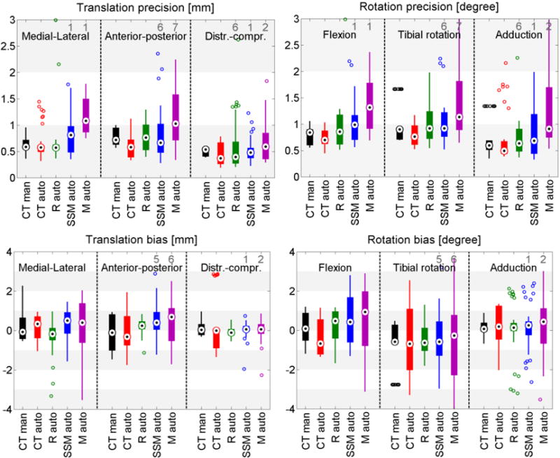
Box plots of the kinematic precision (1st row) and bias (2nd row) with all methods on the cadaveric datasets. Results are relative to the gold standard marker based kinematics. The black dots represent the median value, wide lines indicate the 25th and 75th percentiles, and whiskers extend to the most extreme data points not considered outliers. Outliers are plotted individually as circles, and the number of outliers outside the axis range is shown in gray numbers.
Experiment 2 focused on the relationship between shape accuracy and kinematic precision by calculating kinematics with shapes of varying quality: the CT shape, being ground truth; the SSM representation of the CT shape with an average accuracy of 0.63 mm and 0.85 mm; the SSM mean shape with an average accuracy of 1.37 mm; and 1.64 mm; and the SSM-based 2D/3D reconstruction with an average accuracy of 1.18 mm and 1.56 mm, for the femur and tibia-fibula. Results in Figure 4 show an average trend of better kinematic precision with more accurate shapes. Figure 5 depicts the shape accuracy versus kinematic accuracy per subject and per initialization. We defined the total kinematic accuracy for this figure as the norm of the kinematic precision (in mm and degrees), and the average shape accuracy as the mean accuracy of the femur and the tibia-fibula. This figure illustrates that on the individual level a better shape accuracy does not necessarily result in better kinematic accuracy, e.g. the SSM reconstruction (Rauto) in cadaver 2 has half the shape error as the 2D/3D reconstruction (SSMauto), yet its kinematic accuracy is worse. Similar conclusions can be drawn from Cadaver 1 and 6.
Figure 5.
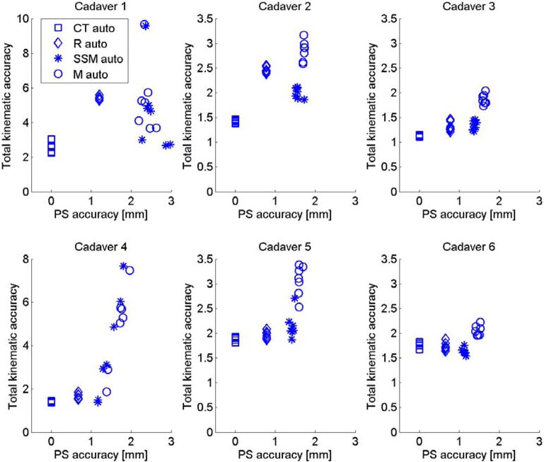
Kinematic accuracy of all six cadavers versus average point-to-surface (PS) shape accuracy (average over femur and tibia) with different models.
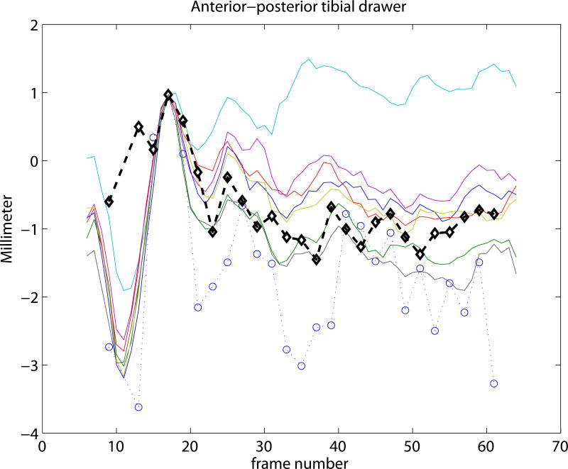
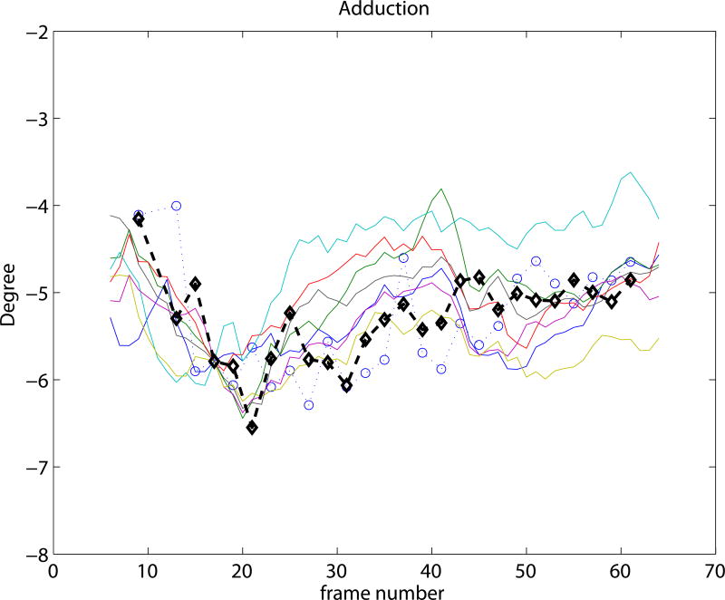
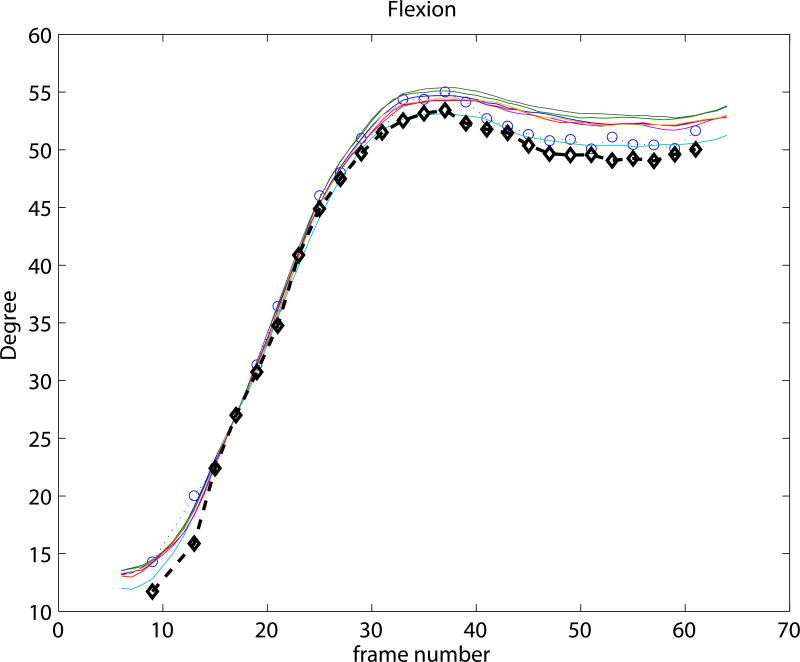
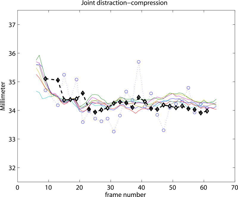
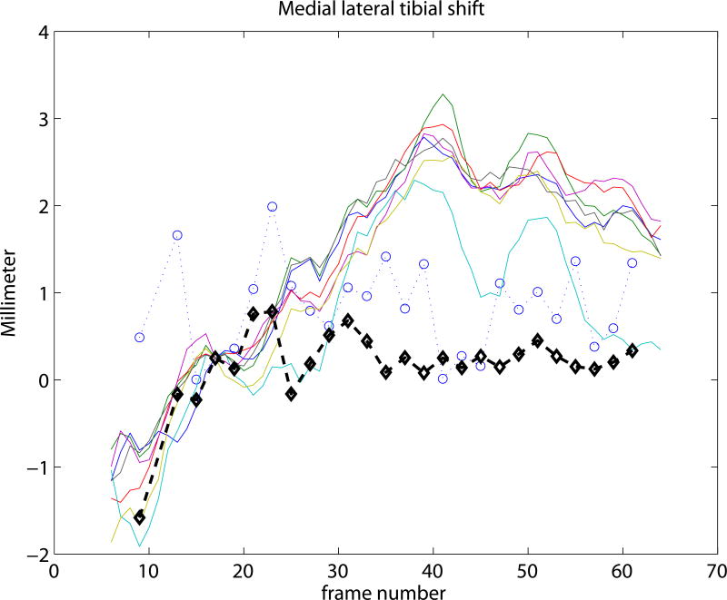
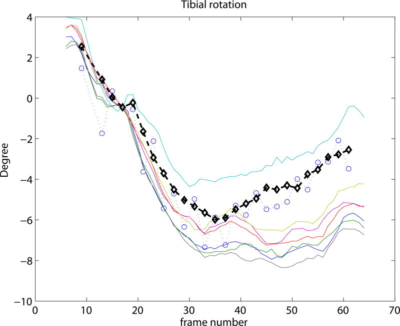
Experiment 3 focused on the evaluation of the SSM based knee kinematics in the in-vivo as well as cadaver datasets. Results on the cadaveric sequences are presented in Figure 4 compared to marker based kinematics, and in Table 1 compared to markers as well as to CTman. Results show a sub-millimeter (0.48-0.81 mm) and approximately one degree (0.69-0.99°) median precision compared to markers. Evaluating against the CTman gave on average 0.12 mm and 0.18° higher precision errors, due to the lower accuracy of CTman. The most difficult parameter to estimate was the tibial rotation, inhabiting the largest 95 percentile precision as well as bias errors. Typical time-curves of marker-based kinematics, CTman kinematics, and SSMauto kinematics with the seven different initializations are shown in Figure 7 Results on the in-vivo datasets are reported in Table 2, showing comparable bias and precision values as the cadaver cases. Figure 6 shows an example frame from an in-vivo sequence, with reconstructed bones and their projections on the images.
Table 1.
Results of the SSM-based kinematics on the cadaver sequences, evaluated against marker-based kinematics and against the reference method CTman. We report the median [5 and 95 percentiles].
| SSM vs Markers | SSM vs CTman | |||
|---|---|---|---|---|
| bias | precision | bias | precision | |
| flexion (°) | 0.42[-1.26, 2.33] | 0.99[0.59, 2.15] | 0.42[-0.88, 1.96] | 0.94[0.42, 1.90] |
| tibial rotation (°) | -0.58[-4.36, 6.56] | 0.92[0.62, 4.23] | -0.20[-1.83, 6.28] | 1.28[0.78, 4.40] |
| adduction (°) | 0.26[-1.77, 2.31] | 0.69[0.35, 1.98] | -0.20[-1.84, 2.97] | 0.73[0.57, 3.02] |
| ML tibial shift (mm) | 0.51[-0.99, 1.39] | 0.81[0.40, 1.73] | 0.45[-2.32, 1.47] | 0.89[0.59, 1.79] |
| AP tibial drawer (mm) | 0.40[-0.49, 2.02] | 0.66[0.31, 2.18] | 1.04[-0.96, 2.05] | 0.92[0.62, 2.13] |
| joint distr-contr (mm) | 0.06[-0.52, 0.46] | 0.48[0.25, 1.13] | -0.09[-1.14, 0.73] | 0.70[0.47, 1.31] |
Figure 7.
Kinematic curves of one cadaver knee. Marker based gold standard kinematics is shown with black diamonds, the CTman reference method is shown with blue circles, and the SSMauto results with 7 different random initializations are plotted in various colors. Coordinate systems were linked at frame 17.
Table 2.
Results of the SSM-based kinematics on the in-vivo fluoroscopic data, evaluated against the reference method CTman. We report the median [5 and 95 percentiles].
| SSM vs CTman | ||
|---|---|---|
| bias | precision | |
| Flexion (°) | 0.32[-1.10, 2.20] | 0.95[0.54, 2.85] |
| Tibial rotation (°) | -0.18[-3.81, 2.28] | 1.18[0.89, 3.34] |
| Adduction (°) | -0.51[-1.22, 1.33] | 1.21[0.65, 4.29] |
| ML tibial shift (mm) | 0.05[-1.87, 1.73] | 0.83[0.48, 1.28] |
| AP tibial drawer (mm) | -0.28[-1.36, 1.58] | 0.96[0.51, 2.11] |
| joint distr-contr (mm) | -0.07[-0.36, 0.98] | 0.61[0.34, 0.95] |
Figure 6.
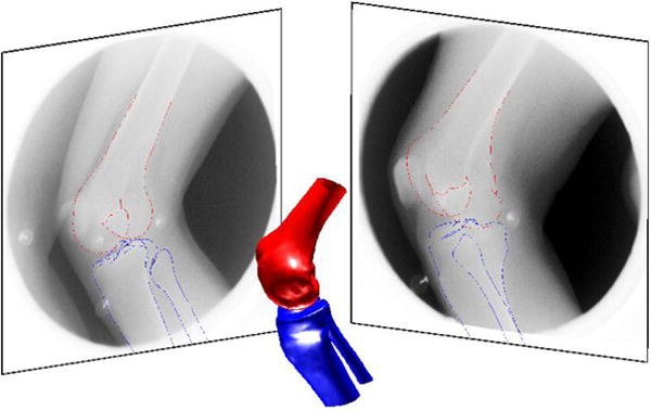
An example bi-plane frame from the in-vivo drop-landing data with SSM based shape reconstruction, and its projection on the fluoroscopic frames. Shape reconstruction accuracy of this example was 1.18 mm for the femur and 1.56 mm for the tibia.
Discussion
In this study we investigated the performance of statistical shape models for deriving fluoroscopy based joint kinematics. Two questions were inspected: Does the accuracy of the surface reconstruction influence kinematics? And what kinematic accuracy can we achieve with the automated SSM method? These questions were answered in three experiments comparing the obtained kinematics with marker-based kinematics in six cadaver datasets, and with a CT segmentation-based manual interaction intensive CTman method in ten in-vivo cases.
All SSM based methods used automated edge selection. To separate the effect of edge selection type and surface-model type, we first tested the edge selection separately. We found in experiment 1, that with the CT-derived bone shapes both manual (CTman) and automated edge selection (CTauto) methods gave a sub-millimeter and sub-degree precision (Figure 4), in accordance with (Giphart et al., 2012). CTauto showed a lower median precision error, but larger bias. This is probably because the marker coordinate-system was linked with the coordinate-system of the CT-derived bone at a chosen frame using the CTman bone position. Any pose difference between CTman and CTauto in that frame creates bias for the automated method. For one cadaver the CTauto method failed (outliers in Figure 4). In this severely arthritic knee the automatic edge detection for the tibia-fibula failed due to too many spurious edges. Overall, we conclude that automated edge selection is a valid alternative to manual kinematic analysis.
In experiment 2 we analyzed the relationship between shape accuracy and kinematic precision using automated edge selection. Figure 4 demonstrates that the median kinematic precision improved with improving shape accuracy. However, Figure 5 illustrates that this relationship does not hold on the individual level. This suggests that the ability to fit the edges in the fluoroscopic sequences has a larger role in determining the kinematic precision than the overall 3D shape accuracy.
In experiment 3 we evaluated the proposed automated SSM-based kinematics method on cadavers as well as in-vivo data. A sub-millimeter (0.48-0.81 mm) and approximately one degree (0.69-0.99°) median tracking precision was achieved compared to marker-based kinematics, though in individual cases this precision was worse (Figure 4, Table 1). The in-vivo sequences were only evaluated against CTman. Resulting precision values were comparable with the cadaver sequences when evaluated against CTman (Table 1, 2). This suggests that cadaveric and in-vivo tracking performance was similar. The spread in kinematic accuracy with different starting positions was larger with SSMauto than with CTauto (Figure 4, 5). This may be due to the selection of wrong edges in the fitting process. In clinical use, assessment of the tracking quality is therefore important. Nevertheless, these results are encouraging, as they indicate that the SSM may be able to replace the subject-specific bone shapes for kinematic analysis.
In the current study the kinematic precision was calculated from an entire sequence, with the joint entering and leaving the FOV. Pose estimation and thereby tracking, was though more accurate in the middle of the sequence where all characteristic parts of the bone were visible in the FOV, i.e. both condyles and a few cm of the shaft for the femur, and the entire tibial plateau, the fibula, and a few cm-s of the shaft for the tibia. Automated SSM-based kinematics of different motions (e.g. knee bend) may therefore perform better.
In the current study the coordinate-systems of the CT segmented bones were linked to the SSM in a pre-chosen frame of each sequence. This is illustrated in Figure 7, where all curves cross each other at frame 17. Such choice of coordinate-system linkage is arbitrary, and propagates the misalignment at the pre-chosen frame to the rest of the sequence, causing bias (see e.g. the flexion parameter in Figure 7). Coordinate-system definitions may greatly influence the results (Lenz et al., 2008), but analyzing the effect is outside the scope of this paper.
The shape reconstruction accuracy with SSMauto is comparable with other state-of-the-art methods on the femur bone (little work has been done on tibia-fibula reconstruction in the literature). Reported RMS point-to-surface (PS) distances for the femur were 0.99 mm using simulated silhouettes (Fleute and Lavallée, 1999), 1.4 mm using semi-automated region selected contours (Laporte et al., 2003), and 1.43 mm RMS PS distance on similar jump-landing sequences (Baka et al., 2012). A mean PS distance of 0.90 mm was reported when fitting to the bone silhouette from the X-ray images (Zhu and Li, 2011). The pose independent shape reconstruction accuracy of the femur in this study was 1.18 mm RMS PS distance, and 0.95 mm mean PS distance.
Calculating the SSM-based knee kinematics in an un-optimized Matlab implementation took 2 hours on a 2.26 GHz processor with 24 GB memory, including tracking and reconstruction of both tibia and femur.
Limitations of the method include the fact that the SSM was trained on asymptomatic subjects. Subjects with bone deformities (such as Cadaver 1 in this study) will not be represented well by the current model, and are expected to have worse kinematic accuracies. Most studies are though performed to assess knee kinematics without severe bone pathology and pathology-specific SSMs may be developed in the future.
Future work may focus on making SSM-based kinematics more robust. This could be achieved by reducing spurious edges in the X-ray images for example by semi-automatically delineating desired edges in one frame, and automatically tracking these edges through the sequence.
In conclusion, this study investigated the applicability of statistical shape models for calculating knee joint kinematics from biplane fluoroscopic sequences, which could potentially obsolete prior 3D CT/MR acquisitions. We demonstrated that an SSM-based automated method can achieve sub-millimeter median precision for translations and approximately one degree median precision for rotations. These results are promising, though further work is necessary to reach the accuracy of CT-based kinematics. We also demonstrated that a better shape reconstruction accuracy does not automatically imply a better kinematic precision. This result suggests that the ability of accurately fitting the edges in the fluoroscopic sequences has a larger role in determining the kinematic precision than the overall 3D shape accuracy.
Acknowledgments
This study was financed by the European Community (MXL project 248693), NIH funding AR39683, and NWO grant number 612.065.618. We thank SARA Computing and Networking Services (www.sara.nl) for their support in using the Lisa Compute Cluster.
Footnotes
Due to the higher frame rate of our fluoroscopic sequences, we omitted the edge appearance terms proposed to enable tracking from low frame-rate sequences.
Taking a subset of frames was advantageous for increasing speed, and improving shape reconstruction by excluding frames containing only a small portion of the bone.
in clinical use manual initialization with such accuracy can be easily accomplished e.g. by manually selecting the object edges to fit the model to in the start frame.
There is no conflict of interest.
Publisher's Disclaimer: This is a PDF file of an unedited manuscript that has been accepted for publication. As a service to our customers we are providing this early version of the manuscript. The manuscript will undergo copyediting, typesetting, and review of the resulting proof before it is published in its final citable form. Please note that during the production process errors may be discovered which could affect the content, and all legal disclaimers that apply to the journal pertain.
References
- Anderst W, Zauel R, Bishop J, Demps E, Tashman S. Validation of three-dimensional model-based tibio-femoral tracking during running. Medical engineering & physics. 2009;31:10–6. doi: 10.1016/j.medengphy.2008.03.003. [DOI] [PMC free article] [PubMed] [Google Scholar]
- Baka N, de Bruijne M, van Walsum T, Kaptein B, Giphart J, Schaap M, Niessen W, Lelieveldt B. Statistical Shape Model Based Femur Kinematics from Biplane Fluoroscopy. IEEE Transactions on Medical Imaging. 2012;31:1573–83. doi: 10.1109/TMI.2012.2195783. [DOI] [PubMed] [Google Scholar]
- Baka N, Kaptein BL, de Bruijne M, van Walsum T, Giphart JE, Niessen WJ, Lelieveldt BPF. 2D-3D shape reconstruction of the distal femur from stereo X-ray imaging using statistical shape models. Medical Image Analysis. 2011;15:840–850. doi: 10.1016/j.media.2011.04.001. [DOI] [PubMed] [Google Scholar]
- Bey MJ, Kline SK, Tashman S, Zauel R. Accuracy of biplane x-ray imaging combined with model-based tracking for measuring in-vivo patellofemoral joint motion. Journal of orthopaedic surgery and research. 2008;3:38. doi: 10.1186/1749-799X-3-38. [DOI] [PMC free article] [PubMed] [Google Scholar]
- Canny J. A Computational Approach to Edge Detection. IEEE Transactions on Pattern Analysis and Machine Intelligence. 1986;PAMI-8:679–698. [PubMed] [Google Scholar]
- Chen X, Graham J, Hutchinson C, Muir L. Inferring 3D Kinematics of Carpal Bones from Single View Fluoroscopic Sequences. In: Fichtinger G, Martel A, Peters T, editors. MICCAI 2011, Medical Image Computing and Computer-Assisted Intervention. Springer Berlin Heidelberg; Berlin, Heidelberg: 2011. pp. 680–687. [DOI] [PubMed] [Google Scholar]
- Cootes TF, Cooper DH, Taylor CJ, Graham J. Trainable method of parametric shape description. Image and Vision Computing. 1992;10:289–294. [Google Scholar]
- Defrate LE, Papannagari R, Gill TJ, Moses JM, Pathare NP, Li G. The 6 degrees of freedom kinematics of the knee after anterior cruciate ligament deficiency: an in vivo imaging analysis. The American journal of sports medicine. 2006;34:1240–6. doi: 10.1177/0363546506287299. [DOI] [PubMed] [Google Scholar]
- Dennis DA, Mahfouz MR, Komistek RD, Hoff W. In vivo determination of normal and anterior cruciate ligament-deficient knee kinematics. Journal of biomechanics. 2005;38:241–53. doi: 10.1016/j.jbiomech.2004.02.042. [DOI] [PubMed] [Google Scholar]
- Fleute M, Lavallée S. Nonrigid 3-D/2-D Registration of Images Using Statistical Models. MICCAI '99: Proceedings of the Second International Conference on Medical Image Computing and Computer-Assisted Intervention; London, UK. 1999. pp. 138–147. [Google Scholar]
- Fregly BJ, Rahman HA, Banks SA. Theoretical Accuracy of Model-Based Shape Matching for Measuring Natural Knee Kinematics with Single-Plane Fluoroscopy. Journal of Biomechanical Engineering. 2005;127:692–699. doi: 10.1115/1.1933949. [DOI] [PMC free article] [PubMed] [Google Scholar]
- Gamage P, Xie SQ, Delmas P, Xu P. Proceedings of the 2009 Digital Image Computing: Techniques and Applications. IEEE Computer Society; Washington, DC, USA: 2009. 3D Reconstruction of Patient Specific Bone Models from 2D Radiographs for Image Guided Orthopedic Surgery; pp. 212–216. [Google Scholar]
- Garling EH, Kaptein BL, Mertens B, Barendregt W, Veeger HEJ, Nelissen RGHH, Valstar ER. Soft-tissue artefact assessment during step-up using fluoroscopy and skin-mounted markers. Journal of biomechanics. 2007;40(Suppl 1):S18–24. doi: 10.1016/j.jbiomech.2007.03.003. [DOI] [PubMed] [Google Scholar]
- Giphart JE, Shelburne KB, Anstett K, Brunkhorst JP, Pault JD, Woo SLY, Steadman JR, Torry MR. Measurement of 3D In Vivo Knee Motion Using Biplane Fluoroscopy: Investigation of Non-contact ACL Injuries. 16th International Conference on Mechanics in Medicine and Biology; 2008. pp. 23–25. [Google Scholar]
- Giphart JE, Zirker CA, Myers CA, Pennington WW, Laprade RF. Accuracy of a contour-based biplane fluoroscopy technique for tracking knee joint kinematics of different speeds. Journal of biomechanics. 2012;45:2935–8. doi: 10.1016/j.jbiomech.2012.08.045. [DOI] [PubMed] [Google Scholar]
- Gollmer ST, Lachner R, Buzug TM. Registration algorithm for statistical bone shape reconstruction from radiographs - an accuracy study. Annual International Conference of the IEEE Engineering in Medicine and Biology Society; 2007. pp. 6376–9. [DOI] [PubMed] [Google Scholar]
- Grood ES, Suntay WJ. A joint coordinate system for the clinical description of three-dimensional motions: application to the knee. Journal of biomechanical engineering. 1983;105:136–44. doi: 10.1115/1.3138397. [DOI] [PubMed] [Google Scholar]
- Hanson GR, Suggs JF, Freiberg AA, Durbhakula S, Li G. Investigation of in vivo 6DOF total knee arthoplasty kinematics using a dual orthogonal fluoroscopic system. Journal of orthopaedic research : official publication of the Orthopaedic Research Society. 2006;24:974–81. doi: 10.1002/jor.20141. [DOI] [PubMed] [Google Scholar]
- Hirokawa S, Abrar Hossain M, Kihara Y, Ariyoshi S. A 3D kinematic estimation of knee prosthesis using X-ray projection images: clinical assessment of the improved algorithm for fluoroscopy images. Medical & biological engineering & computing. 2008;46:1253–62. doi: 10.1007/s11517-008-0398-8. [DOI] [PubMed] [Google Scholar]
- Kitagawa A, Tsumura N, Chin T, Gamada K, Banks SA, Kurosaka M. In vivo comparison of knee kinematics before and after high-flexion posterior cruciate-retaining total knee arthroplasty. The Journal of arthroplasty. 2010;25:964–9. doi: 10.1016/j.arth.2009.07.008. [DOI] [PubMed] [Google Scholar]
- Klein S, Staring M, Murphy K, Viergever MA, Pluim JPW. elastix: a toolbox for intensity-based medical image registration. IEEE Transactions on Medical Imaging. 2010;29:196–205. doi: 10.1109/TMI.2009.2035616. [DOI] [PubMed] [Google Scholar]
- Laporte S, Skalli W, de Guise JA, Lavaste F, Mitton D. A Biplanar Reconstruction Method Based on 2D and 3D Contours: Application to the Distal Femur. Computer Methods in Biomechanics and Biomedical Engineering. 2003;6:1–6. doi: 10.1080/1025584031000065956. [DOI] [PubMed] [Google Scholar]
- Lenz NM, Mane A, Maletsky LP, Morton NA. The Effects of Femoral Fixed Body Coordinate System Definition on Knee Kinematic Description. Journal of biomechanical engineering. 2008;130:021014. doi: 10.1115/1.2898713. [DOI] [PubMed] [Google Scholar]
- Li G, Defrate LE, Rubash HE, Gill TJ. In vivo kinematics of the ACL during weight-bearing knee flexion. Journal of orthopaedic research : official publication of the Orthopaedic Research Society. 2005;23:340–4. doi: 10.1016/j.orthres.2004.08.006. [DOI] [PubMed] [Google Scholar]
- Li G, Van de Velde SK, Bingham JT. Validation of a non-invasive fluoroscopic imaging technique for the measurement of dynamic knee joint motion. Journal of biomechanics. 2008;41:1616–22. doi: 10.1016/j.jbiomech.2008.01.034. [DOI] [PubMed] [Google Scholar]
- Mahalanobis PC. On the generalised distance in statistic. Proceedings of the National Institute of Sciences of India. 1936;2(1):49–55. [Google Scholar]
- Mahfouz MR, Hoff WA, Komistek RD, Dennis DA. A robust method for registration of three-dimensional knee implant models to two-dimensional fluoroscopy images. IEEE transactions on medical imaging. 2003;22:1561–74. doi: 10.1109/TMI.2003.820027. [DOI] [PubMed] [Google Scholar]
- Miranda DL, Rainbow MJ, Leventhal EL, Crisco JJ, Fleming BC. Automatic determination of anatomical coordinate systems for three-dimensional bone models of the isolated human knee. Journal of Biomechanics. 2010;43:1623–1626. doi: 10.1016/j.jbiomech.2010.01.036. [DOI] [PMC free article] [PubMed] [Google Scholar]
- Moewis P, Wolterbeek N, Diederichs G, Valstar E, Heller MO, Taylor WR. The quality of bone surfaces may govern the use of model based fluoroscopy in the determination of joint laxity. Medical engineering & physics. 2012;34:1427–32. doi: 10.1016/j.medengphy.2012.01.007. [DOI] [PubMed] [Google Scholar]
- Moro-oka T, Hamai S, Miura H, Shimoto T, Higaki H, Fregly BJ, Iwamoto Y, Banks SA. Can magnetic resonance imaging-derived bone models be used for accurate motion measurement with single-plane three-dimensional shape registration? Journal of orthopaedic research : official publication of the Orthopaedic Research Society. 2007;25:867–72. doi: 10.1002/jor.20355. [DOI] [PubMed] [Google Scholar]
- Muhit AA, Pickering MR, Ward T, Scarvell JM, Smith PN. A comparison of the 3D kinematic measurements obtained by single-plane 2D-3D image registration and RSA. Annual International Conference of the IEEE Engineering in Medicine and Biology Society; 2010. pp. 6288–91. [DOI] [PubMed] [Google Scholar]
- Nakajima Y, Tashiro T, Sugano N, Yonenobu K, Koyama T, Maeda Y, Tamura Y, Saito M, Tamura S, Mitsuishi M, Sugita N, Sakuma I, Ochi T, Matsumoto Y. Fluoroscopic bone fragment tracking for surgical navigation in femur fracture reduction by incorporating optical tracking of hip joint rotation center. IEEE transactions on bio-medical engineering. 2007;54:1703–6. doi: 10.1109/TBME.2007.900822. [DOI] [PubMed] [Google Scholar]
- Pickering MR, Muhit AA, Scarvell JM, Smith PN. A new multi-modal similarity measure for fast gradient-based 2D-3D image registration. Annual International Conference of the IEEE Engineering in Medicine and Biology Society; 2009. pp. 5821–4. [DOI] [PubMed] [Google Scholar]
- Scott C, Barney Smith EH. 19th IEEE Symposium on Computer-Based Medical Systems (CBMS'06) IEEE. 2006. An Unsupervised Fluoroscopic Analysis of Knee Joint Kinematics; pp. 377–381. [Google Scholar]
- Stagni R, Fantozzi S, Cappello A, Leardini A. Quantification of soft tissue artefact in motion analysis by combining 3D fluoroscopy and stereophotogrammetry: a study on two subjects. Clinical biomechanics (Bristol, Avon) 2005;20:320–9. doi: 10.1016/j.clinbiomech.2004.11.012. [DOI] [PubMed] [Google Scholar]
- Tashman S, Anderst W. In-Vivo Measurement of Dynamic Joint Motion Using High Speed Biplane Radiography and CT: Application to Canine ACL Deficiency. Journal of Biomechanical Engineering. 2003;125:238–245. doi: 10.1115/1.1559896. [DOI] [PubMed] [Google Scholar]
- Tersi L, Barré A, Fantozzi S, Stagni R. In vitro quantification of the performance of model-based mono-planar and bi-planar fluoroscopy for 3D joint kinematics estimation. Medical & biological engineering & computing. 2012:1–9. doi: 10.1007/s11517-012-0987-4. [DOI] [PubMed] [Google Scholar]
- Torry MR, Myers C, Pennington WW, Shelburne KB, Krong JP, Giphart JE, Steadman JR, Woo SLY. Relationship of anterior knee laxity to knee translations during drop landings: a bi-plane fluoroscopy study. Knee surgery, sports traumatology, arthroscopy : official journal of the ESSKA. 2011;19:653–62. doi: 10.1007/s00167-010-1327-6. [DOI] [PMC free article] [PubMed] [Google Scholar]
- Torry MR, Shelburne KB, Peterson DS, Giphart JE, Krong JP, Myers C, Steadman JR, Woo SLY. Knee Kinematic Profiles During Drop Landings: A Biplane Fluoroscopy Study. Medicine and science in sports and exercise. 2010;43:533–41. doi: 10.1249/MSS.0b013e3181f1e491. [DOI] [PubMed] [Google Scholar]
- Tsai TY, Lu TW, Chen CM, Kuo MY, Hsu HC. A volumetric model-based 2D to 3D registration method for measuring kinematics of natural knees with single-plane fluoroscopy. Medical physics. 2010;37:1273–84. doi: 10.1118/1.3301596. [DOI] [PubMed] [Google Scholar]
- Whitmarsh T, Humbert L, De Craene M, Del Rio Barquero LM, Frangi AF. Reconstructing the 3D shape and bone mineral density distribution of the proximal femur from dual-energy X-ray absorptiometry. IEEE transactions on medical imaging. 2011;30:2101–14. doi: 10.1109/TMI.2011.2163074. [DOI] [PubMed] [Google Scholar]
- You BM, Siy P, Anderst W, Tashman S. In vivo measurement of 3-D skeletal kinematics from sequences of biplane radiographs: application to knee kinematics. IEEE transactions on medical imaging. 2001;20:514–25. doi: 10.1109/42.929617. [DOI] [PubMed] [Google Scholar]
- Zheng G, Gollmer S, Schumann S, Dong X, Feilkas T, Ballester MAG. A 2D/3D correspondence building method for reconstruction of a patient-specific 3D bone surface model using point distribution models and calibrated X-ray images. Medical Image Analysis. 2008;13(6):883–899. doi: 10.1016/j.media.2008.12.003. [DOI] [PubMed] [Google Scholar]
- Zhu Z, Li G. Construction of 3D human distal femoral surface models using a 3D statistical deformable model. Journal of biomechanics. 2011;44:2368–2362. doi: 10.1016/j.jbiomech.2011.07.006. [DOI] [PMC free article] [PubMed] [Google Scholar]


