Social interactions dominate speed control in poising natural flocks near criticality

Significance

The coherent flight of bird flocks is one of nature’s most impressive aerial displays. Beyond the fact that thousands of birds fly, on average, with the same velocity, quantitative observations show that small deviations of individual birds from this average are correlated across the entire flock. By learning minimally structured models from field data, we show that these long-ranged correlations are consistent with local interactions among neighboring birds, but only because the parameters of the flock are tuned to special values, mathematically equivalent to a critical point in statistical mechanics. Being in this critical regime allows information to propagate almost without loss throughout the flock, while keeping the variance of individual velocities small.

Abstract

Flocks of birds exhibit a remarkable degree of coordination and collective response. It is not just that thousands of individuals fly, on average, in the same direction and at the same speed, but that even the fluctuations around the mean velocity are correlated over long distances. Quantitative measurements on flocks of starlings, in particular, show that these fluctuations are scale-free, with effective correlation lengths proportional to the linear size of the flock. Here we construct models for the joint distribution of velocities in the flock that reproduce the observed local correlations between individuals and their neighbors, as well as the variance of flight speeds across individuals, but otherwise have as little structure as possible. These minimally structured or maximum entropy models provide quantitative, parameter-free predictions for the spread of correlations throughout the flock, and these are in excellent agreement with the data. These models are mathematically equivalent to statistical physics models for ordering in magnets, and the correct prediction of scale-free correlations arises because the parameters—completely determined by the data—are in the critical regime. In biological terms, criticality allows the flock to achieve maximal correlation across long distances with limited speed fluctuations.

In a flock of birds, thousands of individuals will fly in the same direction and at the same speed, for long periods of time. However, this average behavior is not enough for flocking to be advantageous. The entire flock must respond to dangers that may be visible only to a small fraction of individuals, requiring information to propagate over long distances. Although it is difficult to measure this information flow directly (1), we know that attacks by predators on a flock have very low success rates (2–4), and that the evasion of predators by starling flocks is associated with the triggering and propagation of waves through the flock (5). Even in the absence of predators, we can see deviations of individual behavior from the average behavior of the flock, and correlations in these fluctuations provide a signature of information flow through the flock. Strikingly, observations on flocks of starlings show that these correlations extend over very long distances, comparable to the size of the flock itself (6).

It is generally believed that the interactions among birds in a flock are local—each bird aligns its flight direction and speed to those of its near neighbors (7). If this is correct, then we have to understand how local interactions can generate correlations over much longer distances. In physics, we have two very different mechanisms for local interactions to produce long–ranged correlations. If the system spontaneously breaks a continuous symmetry, for example when all of the spins in a magnet select a particular direction in space along which the macroscopic magnetization will point, then the fluctuations in the system are dominated by Goldstone modes that do not decay on any fixed length scale (8). If we can think of the alignment of flight directions in a flock as being like the alignment of spins in a magnet (9–11), then we can understand the emergence of scale-free correlations via Goldstone’s theorem. We have shown that this is more than a metaphor (12): the minimally structured model consistent with the observed correlations among flight directions of neighboring birds is equivalent to a model of spins in a magnet, and the resulting (parameter-free) prediction of long-ranged correlations among fluctuations in flight direction agrees quantitatively with the data.

Not just the fluctuations in flight direction, but also the fluctuations in flight speed are correlated over long distances (6). Now there are no Goldstone modes, because choosing a speed does not correspond to breaking any plausible symmetry of the system. However, there is a second mechanism by which physical systems generate scale-free correlations, and this is by tuning parameters to a critical point (8, 13). As we explore the parameter space of a system (e.g., changing temperature and pressure), we encounter phase transitions, where small changes in parameters produce qualitative changes in behavior of a macroscopic sample (e.g., between liquid and gas). Along the lines in parameter space where these phase transitions exist, there are special points, called “critical points,” where the dependence on parameters becomes, for very large systems, singular but not discontinuous. At these points, fluctuations (e.g., in the density of the liquid) become correlated on all length scales, from the molecular scale of the interactions to the macroscopic scale of the sample as a whole.

Tuning to a critical point provides a potential explanation for scale-free correlations in speed of flocking birds, but this is just an analogy; the goal of this paper is to construct a quantitative theory. Our strategy follows ref. 12: we construct the least structured models that are consistent with measured correlations among neighboring birds, and then see if these models can correctly predict the persistence of correlations over much longer distances, comparable to the size of the flock. We will see that this works, and that the underlying mechanism really is the tuning of the system to a critical point. From a biological point of view, this means that individuals in a flock combine individual speed control and social interactions with their neighbors to achieve a maximal range of influence while keeping speed variability low.

Building a Model from Data

We consider flocks of European starlings, Sturnus vulgaris, in the field. The work of refs. 14 and 15 provides a detailed description of these flocks, resulting in the assignment of 3D positions and velocities, at each moment in time, to each individual bird in flocks with up to several thousand members (for a summary, see SI Text, section I). From these raw data, one can extract a variety of features that serve to characterize the nature of the ordering in the flock (6, 16).

The positions and velocities of all of the birds in the flock are stochastic—with elements of randomness, but correlated. In making a model, we want to predict the probability distribution out of which these random variables are drawn. One approach is to consider a detailed model for the dynamics of the flock, typically with many parameters to describe the interactions that cause the flock to cohere and align. However, the connection between the model dynamics and the joint distribution of velocities in the flock can be complicated, and fitting the parameters of the interactions is difficult (17); there also is a problem of whether we should take such models seriously as description of the “microscopic” interactions among individuals, or whether they are to be considered as effective interactions in the spirit of statistical physics. As an alternative, we can take some set of observations on the flock as given and try to construct models that reproduce these observations exactly; among the (generally infinite) set of models that can do this, we want to choose the one that has the least structure. Minimizing structure means that the velocities we choose out of the distribution are as random as they can be while still matching the properties of the flock that we have chosen as essential. As emphasized by Jaynes (18, 19), these minimally structured distributions have maximum entropy, providing a connection to the ideas of statistical physics (SI Text, section II).

A realistic model for a flock might or might not lead to a maximum entropy distribution. Also, the maximum entropy method is not in itself a model: to use the method we have to choose some set of experimental observations as constraints, and it is easy to imagine choosing the wrong ones. Thus, the maximum entropy approach is a source of hypotheses, and these must be tested. If the maximum entropy model consistent with a limited set of experimental constraints is accurate, correctly predicting experimental observations that were not part of its formulation, then we can take the model seriously and ask what it teaches us about the system.

The maximum entropy approach to model building is far from new, but there has been a resurgence of interest in the use of these ideas to describe biological systems (20–29). In ref. 12, we took a first step toward a maximum entropy description of flocks, building models for the distribution of flight directions that match the average local correlation between the direction of a bird and its nearest neighbors. Surprisingly, fixing this one number leads to a model that, with no free parameters, provides an essentially complete, quantitative description of the propagation of directional order throughout the entire flock. Here we generalize this approach to consider not just flight directions, but also speed. As explained above, we expect that accounting for the properties of speed ordering is a qualitatively different problem from the case of directional ordering.

Given the positions of the birds in space, the state of the flock is defined by the velocity ${\overrightarrow{\mathbf{v}}}_{\text{i}}$ of each bird. This 3D vector is composed of the speed, $v_{\text{i}}\mathrm{\equiv }\left|{\overrightarrow{\mathbf{v}}}_{\text{i}}\right|$, and a unit vector, ${\overrightarrow{\mathbf{s}}}_{\text{i}}={\overrightarrow{\mathbf{v}}}_{\text{i}}/v_{\text{i}}$, that points in the direction of flight. Our intuition is that the most important interactions are local, between a bird and its immediate neighbors. If this is correct, then the essential features of the system should be captured by measuring local correlations, as in ref. 12.

We can quantify local correlations in the flock by asking how similar, on average, the velocity of each bird is to its neighbors. To do this, we define

$$Q_{\text{int}}=\frac{1}{2v_0^{2}N}{\displaystyle \sum _{\text{i}=1}^N\frac{1}{n_c}{\displaystyle \sum _{\text{j}\in {\mathcal{N}}_{\text{i}}}{\left|{\overrightarrow{\mathbf{v}}}_{\text{i}}-{\overrightarrow{\mathbf{v}}}_{\text{j}}\right|}^2}}.$$ [1]

Here ${\mathcal{N}}_{\text{i}}$ is the relevant neighborhood of bird i, which we take to be its first $n_c$ nearest neighbors (12, 16). We compare a bird to each of its neighbors, average over the neighborhood, and then average over all N birds in the flock; we normalize the result by a typical speed $v_0$ so that we have a dimensionless measure of correlation or similarity. If we take $v_0$ to be the average speed of birds in the flock, then typical values for $Q_{\text{int}}$ are $\sim {10}^{-2}$ (Table S1), showing that birds indeed fly with velocities very similar to those of their neighbors.

The definition of $Q_{\text{int}}$ quantifies the similarity of each bird’s flight vector to that of its neighbors, but if we add a constant to all of the velocities, so that the flock flies faster or slower, then $Q_{\text{int}}$ is unchanged. We would like to fix the average speed of the birds in the flock, $V=(1/N){\displaystyle {\sum }_{\text{i}=1}^N{v}_{\text{i}}}$, to its observed value ${\langle V\rangle }_{\text{exp}}$. In addition, we know that individual birds have speeds that vary around the mean, so we would also like to match the variance of speeds. This is equivalent to fixing the mean square speed, $V_2=(1/N){\displaystyle {\sum }_{\text{i}=1}^N{v}_{\text{i}}^2}$. In what follows, we will refer also to the fractional variance in speed,

$${\sigma }^2=\frac{1}{N{V}^2}{\displaystyle \sum _{\text{i}=1}^N{\left(v_{\text{i}}-V\right)}^2}.$$ [2]

The maximum entropy distribution consistent with measured values of $Q_{\text{int}}$, V, and $V_2$ has the form (SI Text, section III),

$$\begin{array}{r}P\left(\left\{{\overrightarrow{\mathbf{v}}}_{\text{i}}\right\}\right)=\frac{1}{Z}\exp [-\frac{J}{4v_0^2}{\displaystyle \sum _{\text{ij}=1}^N{n}_{\text{ij}}{\left|{\overrightarrow{\mathbf{v}}}_{\text{i}}-{\overrightarrow{\mathbf{v}}}_{\text{j}}\right|}^2}+\frac{\mu }{v_0}{\displaystyle \sum _{\text{i}=1}^N{v}_{\text{i}}}-\frac{g}{2v_0^2}{\displaystyle \sum _{\text{i}=1}^N{v}_{\text{i}}^2}],\end{array}$$ [3]

where Z is a constant that ensures the normalization of the probability distribution, and we have inserted factors of $v_0$ so that other parameters are dimensionless. The matrix $n_{\text{ij}}$ maps the connections between birds: ${\widehat{n}}_{\text{ij}}=1$ if bird j is in the neighborhood of bird i ($\text{j}\in {\mathcal{N}}_{\text{i}}$), and zero otherwise; we symmetrize to give $n_{\text{ij}}=\left({\widehat{n}}_{\text{ij}}+{\widehat{n}}_{\text{ji}}\right)/2$. The parameters J, μ, and g must be adjusted so that the average values of $Q_{\text{int}}$, V, and $V_2$ computed from the probability distribution match those observed for the flock; as explained in SI Text, section IV, these computations can be done analytically. The only remaining parameter is the number of relevant neighbors $n_c$, which we fix by requiring that the probability of the observed velocities be as large as possible. We expect that birds on the boundary of the flock will experience different signals than those in the interior; rather than making an explicit model, we fix the velocities of the boundary birds (12), so that Eq. 3 provides a theory for the propagation of order through the flock.

Fig. 1 shows one example of our solution to the inverse problem of determining the parameters J, g, and $n_c$. Importantly, the quantities that we are trying to match are averages over all of the birds in the flock, and so they are determined with small errors even from a single snapshot of the velocities. The parameters in turn are determined very precisely, and are consistent for a single flock across time and across multiple flocking events, as in ref. 12 and SI Text, section V. In particular, values of n_c are independent of the size of the flock (Fig. S1) and of the distance between birds (Fig. S2), supporting the idea that birds interact with a fixed number of neighbors.

Fig. 1.

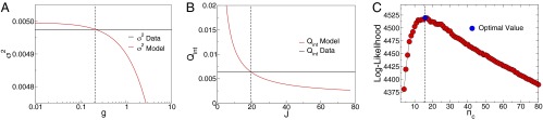
Inference of the three interaction parameters g, J, and $n_c$. (A) For fixed values of J and $n_c$, the value of the speed control parameter g is found by equating the theoretical prediction for the variance of fractional speed fluctuations, ${\sigma }^2$ (red line) from Eq. 2, to its experimental value (black horizontal line). (B) Once the value of g is determined for all possible values of J and $n_c$, the interaction strength J can be set by equating the theoretical prediction for $Q_{\text{int}}$ (red line) to its experimental value (black horizontal line). (C) Once g and J are computed for given values of $n_c$, the log-likelihood of the data, ${\langle \ln P\left(\left\{{\overrightarrow{\mathbf{v}}}_{\text{i}}\right\}\right)\rangle }_{\text{exp}}$ becomes a function of $n_c$ only, and the interaction range $n_c$ can be evaluated by maximizing this function. All panels refer to the same single snapshot of one flock (frame 2 of 25-10 in Tables S1 and S2), and mathematical details can be found in SI Text, section IV.

Some Intuition

Maximum entropy distributions are mathematically equivalent to the Boltzmann distribution for systems in thermal equilibrium, and we can use this identity to gain some intuition for the predictions of the model. We recall that a system described by the Boltzmann distribution will occupy a state s with probability $P_s\propto \exp \left(-E_s/k_{B}T\right)$, where $E_s$ is the energy of the state and $k_{B}T$ is the typical thermal energy; for our purposes we can choose units so that $k_{B}T=1$. Thus, Eq. 3 defines an energy function or Hamiltonian on the space of the birds’ velocities, and this can be written as

$$\mathrm{\mathscr{H}}\left(\left\{{\overrightarrow{\mathbf{v}}}_{\text{i}}\right\}\right)=\frac{J}{4V^2}{\displaystyle \sum _{\text{ij}=1}^N{n}_{\text{ij}}{\left|{\overrightarrow{\mathbf{v}}}_{\text{i}}-{\overrightarrow{\mathbf{v}}}_{\text{j}}\right|}^2}+\frac{g}{2V^2}{\displaystyle \sum _{\text{i}=1}^N{\left(v_{\text{i}}-V\right)}^2},$$ [4]

where we have eliminated the parameter μ in favor of the mean speed V, which is now fixed to its experimental value ${\langle V\rangle }_{\text{exp}}$, and we have set the arbitrary scale $v_0=V$.

The first term in this Hamiltonian describes the tendency of the individual velocities to adjust both direction and modulus to their neighbors, while the second term forces the speed to have, on average, the value V. From this perspective, we can interpret J as the stiffness of an effective “spring” that ties each bird’s velocity to that of its neighbors, and g as the stiffness of a competing spring that ties each speed to the desired mean. Larger J means a tighter connection to the neighbors, and larger g means a tighter individual control over speed.

There are interesting limiting cases that give us a sense for what this model predicts. If the parameter g is very large, then the speed of individual birds hardly fluctuates at all. In this limit, we can rewrite the Hamiltonian as

$$\mathrm{\mathscr{H}}\left(\left\{{\overrightarrow{\mathbf{v}}}_{\text{i}}\right\}\right)\approx {\mathrm{\mathscr{H}}}_{\text{dir}}\left(\left\{{\overrightarrow{\mathbf{s}}}_{\text{i}}\right\}\right)=-\frac{J}{2}{\displaystyle \sum _{\text{ij}=1}^N{n}_{\text{ij}}{\overrightarrow{\mathbf{s}}}_{\text{i}}\cdot {\overrightarrow{\mathbf{s}}}_{\text{j}}}.$$ [5]

This describes the tendency of individual birds to align with their neighbors, and is exactly the model in ref. 12.

If there are nonzero but small fluctuations in speed, then we can write $v_{\text{i}}=V\left(1+{\mathit{ϵ}}_{\text{i}}\right)$, and expand in powers of ϵ. The result (SI Text, section IV) is that

$$\mathrm{\mathscr{H}}\left(\left\{{\overrightarrow{\mathbf{v}}}_{\text{i}}\right\}\right)\approx {\mathrm{\mathscr{H}}}_{\text{dir}}\left(\left\{{\overrightarrow{\mathbf{s}}}_{\text{i}}\right\}\right)+{\mathrm{\mathscr{H}}}_{\text{sp}}\left(\left\{{\mathit{ϵ}}_{\text{i}}\right\}\right),$$ [6]

where the speed Hamiltonian

$${\mathrm{\mathscr{H}}}_{\text{sp}}\left(\left\{{\mathit{ϵ}}_{\text{i}}\right\}\right)=\frac{1}{2}{\displaystyle \sum _{\text{i},\text{j}=1}^N\left(g{\delta }_{\text{ij}}+J{N}_{\text{ij}}\right){\mathit{ϵ}}_{\text{i}}{\mathit{ϵ}}_{\text{j}}},$$ [7]

$$N_{\text{ij}}=-n_{\text{ij}}+{\delta }_{\text{ij}}{\displaystyle \sum _{\text{k}=1}^N{n}_{\text{ik}}}.$$ [8]

Thus, our full model breaks into two pieces, one describing fluctuations in flight direction, and one describing fluctuations in speed. However, the strength of the springs that tie the speed of each bird to that of its neighbors is determined by the same parameter J which enters the description of directional fluctuations in Eq. 5. Thus, we have a unified model for how birds adjust their vector velocities to those of their neighbors, rather than separate models (with separate parameters) for the adjustment of direction and speed.

To get a sense for the structure of ${\mathrm{\mathscr{H}}}_{\text{sp}}$, it is useful to imagine a continuum limit in which the variations in speed from bird to bird are so smooth that we can picture the speed fluctuations as a continuous function of position in the flock, $\mathit{ϵ}\left(\overrightarrow{\mathbf{x}}\right)$. In this limit (SI Text, section VI), we have

$${\mathrm{\mathscr{H}}}_{\text{sp}}\approx \frac{\rho }{2}{\displaystyle \int d^{3}x\left[J{n}_c{r}_c^2{\left(\mathrm{\nabla }\mathit{ϵ}\right)}^2+g{\mathit{ϵ}}^2\left(\overrightarrow{\mathbf{x}}\right)\right]},$$ [9]

where $r_c$ is the typical distance to a neighboring bird, and ρ is the density of the flock. This model predicts that

$$\langle \mathit{ϵ}\left(\overrightarrow{\mathbf{x}}\right)\mathit{ϵ}\left({\overrightarrow{\mathbf{x}}}^{\mathbf{\prime }}\right)\rangle \propto \exp \left(-\left|\overrightarrow{\mathbf{x}}-{\overrightarrow{\mathbf{x}}}^{\mathbf{\prime }}\right|/{\xi }_{\text{bulk}}\right),$$ [10]

where correlation length

$${\xi }_{\text{bulk}}\sim r_c\sqrt{J{n}_c/g}$$ [11]

determines the distance over which the fluctuations in speed will be correlated; the subscript reminds us that we are treating the flock as a bulk material, with no boundaries. In this simple picture, there is a critical point at $g=0$ where the correlation length ${\xi }_{\text{bulk}}$ becomes infinite.

As we have written our model, we need to have $g>0$. On the other side of the critical point at $g=0$, we need to constrain the speed distribution more fully (that is, more than just fixing the mean and the variance) to have a well-normalized distribution of velocities. If we make these extensions, then $g<0$ will describe a flock in which there is a bimodal distribution of speeds, which seems unnatural. Thus, in this case, the critical point likely is also the boundary of the biologically relevant parameter space.

To summarize, J determines the propagation of directional order through the flock, and to describe the speed fluctuations we have only one extra parameter g. The value of g is set by matching the observed variance in speed across the birds in the flock (Fig. 1A). However, J and g also compete to determine the distance over which speed fluctuations will be correlated, Eq. 11. Importantly, we are not free to adjust this correlation length by fitting: either the model gets it right, or it does not.

Scale-Free Correlations

Once the parameters J, g, and $n_c$ are determined (Fig. 1), Eq. 3 provides a model for the joint distribution of velocities for all of the birds in the flock; everything that we compute from this distribution is a parameter-free prediction. We start by measuring the similarity of the vector velocities among birds that are not just nearest neighbors, but are separated by greater distances. By analogy with Eq. 1, we can define

$$Q\left(r\right)=\frac{1}{V^2}{\langle {\left|{\overrightarrow{\mathbf{v}}}_{\text{i}}-{\overrightarrow{\mathbf{v}}}_{\text{j}}\right|}^2\rangle }_{r_{\text{ij}}=r},$$ [12]

where the average is over all pairs of birds separated by a distance $r_{\text{ij}}=r$. The predicted $Q\left(r\right)$ matches the data very closely (Fig. 2A), out to distances comparable to the size of the flock, more than 10 times farther than the nearest neighbors.

Fig. 2.

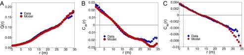
Correlation functions predicted by the maximum entropy model (red circles) vs. experiments (blue diamonds). (A) Similarity of velocities as a function of distance, defined in Eq. 12. The dashed vertical line indicates the size of the neighborhood defined by $n_c$ birds, within which we match the average Q exactly, by construction. (B) Correlations between fluctuations in flight direction as a function of distance, defined in Eq. 14. (C) Correlations between fluctuations in speed as a function of distance, defined in Eq. 15. All panels refer to the same flock and snapshot as in Fig. 1; theoretical predictions are from Eqs. S88–S91.

We next decompose the relationships among velocities into contributions from direction and speed. If we average all of the unit vectors ${\overrightarrow{\mathbf{s}}}_{\text{i}}$ we obtain the overall polarization of the flock,

$$\overrightarrow{\mathbf{P}}=\frac{1}{N}{\displaystyle \sum _{\text{i}=1}^N{\overrightarrow{\mathbf{s}}}_{\text{i}}},$$ [13]

and we can characterize the fluctuations around this overall direction by a correlation function

$$C_{\text{dir}}\left(r\right)={\langle \left({\overrightarrow{\mathbf{s}}}_{\text{i}}-\overrightarrow{\mathbf{P}}\right)\cdot \left({\overrightarrow{\mathbf{s}}}_{\text{j}}-\overrightarrow{\mathbf{P}}\right)\rangle }_{r_{ij}=r}.$$ [14]

In Fig. 2B we compare the data with the predictions of the model, and again find good agreement on all scales.

By analogy with Eq. 14, we can define correlations among the fluctuations in speed,

$$C_{\text{sp}}\left(r\right)={\langle \left(v_{\text{i}}-V\right)\cdot \left(v_{\text{j}}-V\right)\rangle }_{r_{\text{ij}}=r}.$$ [15]

Fig. 2C shows that the observed correlations are in agreement with the predictions of the model, again over the full range of distances. Thus, we have succeeded in constructing a model based on local interactions that generates correlations over long distances, matching the data quantitatively.

The discussion above suggests that long-ranged correlations are associated with the approach to a critical point at $g=0$. To see if this intuition is correct, we show in Fig. 3A what happens to the predicted $C_{\text{sp}}\left(r\right)$ as we change g. Large values of g correspond to small variances in speed, and to correlation functions that decay very rapidly with distance. As g becomes smaller, both the speed variance and the correlation length increase, until, for sufficiently small g, there really is no characteristic scale to the decay of the correlations, and $C_{\text{sp}}\left(r\right)$ is almost a straight line. This is what we observe, and the success of the theory is that the value of g that matches the observed speed variance is in this regime.

Fig. 3.

(A) Correlation function of the speed fluctuations for different values of the control parameter g (increasing in the direction of the arrow). All curves with g less than the optimal value collapse onto the yellow curve. (B) Correlation length, defined as the point where the correlation function crosses zero (6), in flocks of different sizes, for the experimental data (blue diamonds) and for the model (red circles).

We can quantify the approach to criticality by the dimensionless ratio $g/\left(J{n}_c\right)$ that enters Eq. 11. From Fig. 1, we see that $g/\left(J{n}_c\right)\sim {10}^{-3}$, and this is typical (Table S2). This suggests that real flocks are very close to criticality, and that this is why we observe scale-free speed correlations. Note that g cannot be exactly zero, otherwise there is nothing to fix the mean speed of the flock (Eq. 3), and hence the variance in speed relative to a fixed observer (i.e., ground speed) would be infinite. In contrast, the model predicts that the variance of individuals relative to the flock remains finite as $g\to 0$, and the actual value is quite small, ${\sigma }^2\sim 0.005$ in Fig. 1. This measured value of ${\sigma }^2$, together with $Q_{\text{int}}$, fixes the ratio $g/\left(J{n}_c\right)$ to be small enough to generate scale-free correlations.

To be more precise we need to take into account the finite size of the flocks. Eqs. 10 and 11 hold only for an infinite system; for a finite system, the range of the correlation is limited by the system size. As g is lowered, the behavior of the correlations is influenced more and more by these finite size effects: the exponential decay in Eq. 10 is modified, and the typical distance over which correlations extend is no longer described by ${\xi }_{\text{bulk}}$. A more faithful estimate of the correlation length ξ is given instead by the zero of the correlation function (6), and the theoretical prediction depends in a nontrivial way on g and the system size L. For small enough values of g, however, the system is effectively critical, and we should see $\xi \propto L$. In Fig. 3A we show that decreasing g below the level required to match the speed variance of the real flock has essentially no effect, and curves with smaller values of g “pile up” as shown in yellow. Repeating the analysis on flocks of different sizes (Fig. 3B), the correlation length does scale with size, and this pattern is captured perfectly by our maximum entropy models.

We conclude that flocks exhibit critical behavior, being close enough to the critical point to achieve maximum speed correlation length while maintaining a well-defined cruising speed. These conclusions also hold in more general maximum entropy models where speed and flight directions are regulated by different interaction parameters (SI Text, section VII, and Fig. S3).

Dynamical Model

The fact that maximum entropy models are equivalent to the Boltzmann distribution suggests a natural dynamical model, in which the various degrees of freedom in the system execute Brownian motion on the energy landscape:

$$\gamma \frac{d{\overrightarrow{\mathbf{v}}}_{\text{i}}\left(t\right)}{dt}=-{\mathrm{\nabla }}_{\text{i}}\mathrm{\mathscr{H}}\left(\left\{{\overrightarrow{\mathbf{v}}}_{\text{j}}\right\}\right)+{\overrightarrow{\mathit{\eta }}}_{\text{i}}\left(t\right),$$ [16]

where ${\mathrm{\nabla }}_{\text{i}}$ indicates the derivatives with respect to the components of the velocity ${\overrightarrow{\mathbf{v}}}_{\text{i}}$, γ is a constant to set the time scale of the dynamics, and the Langevin force ${\overrightarrow{\eta }}_{\text{i}}\left(t\right)$ is a random, white noise function of time. These dynamics are guaranteed, if the positions of the birds are fixed, to generate velocities that are drawn from the probability distribution in Eq. 3. However, to give a more realistic model we should add to Eq. 16 forces that depend on the positions of the birds (30–32), so as to fix the overall density of the flock (SI Text, section VIII), and the velocities should drive the birds’ positions,

$$\frac{d{\overrightarrow{\mathbf{x}}}_{\text{i}}}{dt}={\overrightarrow{\mathbf{v}}}_{\text{i}}.$$ [17]

Eqs. 16 and 17 define a self-propelled particle model of interacting birds, and is similar to the Vicsek model, so often used to describe flocking particles (33, 34). In contrast to that model and to most of flocking models in the literature, the speed of the individual particles is not fixed, but regulated by the control parameter g.

Simulations of the dynamical model defined by Eqs. 16 and 17 are shown in Fig. 4. As expected from the (static) maximum entropy model, fluctuations in speed have a correlation length that grows as g is reduced. If g is not too small, correlations decay exponentially (Eq. 10), and the correlation length varies with $g/\left(J{n}_c\right)$ as expected. When g is sufficiently small, the exponential decay is modified by finite size corrections, and the correlation length—now computed as the zero-crossing point of the correlation function—keeps decreasing until a maximal, size-dependent saturation value is reached. In this regime, the correlations extend over a distance determined by the system size, and ξ grows linearly with L, corresponding to scale-free behavior (Fig. 4B, Inset). This scenario confirms that the mechanism identified in the previous section produces scale-free correlations in the speed even when the full dynamical behavior of the flock is taken into account.

Fig. 4.

Simulations of a dynamical model (see SI Text, section VIII for details). (A) Correlation function of the speed fluctuations at different values of g in a flock of $N=16\text{,}384$ birds. (Inset) Correlation length, measured from the exponential decay of the correlation functions at small r, as a function of $g/\left(J{n}_c\right)$. (B) For smaller g, correlation lengths are measured from the zero crossing of the correlation function. For $g/\left(J{n}_c\right)\ll 1$, ξ approaches a maximum value that depends on the size of the system. (Inset) Low g maximum of ξ, as a function of the system size; the linear dependence of ξ on L is typical of scale-free behavior.

Conclusions

The understanding of collective behavior in matter at thermal equilibrium provides a touchstone for thinking about emergent phenomena in biological systems. Flocking is an especially attractive example, in which the alignment of birds in a flock reminds us of the alignment of spins in a magnet or molecules in a liquid crystal. However, birds are vastly more complex than spins, and this might be nothing more than a metaphor. The goal of this paper and our previous work (12) has been to show that we can go beyond metaphor, that there is a statistical mechanics description of flocks which makes quantitative, parameter-free predictions that are in detailed agreement with the data.

One dramatic collective phenomenon that can emerge in statistical mechanics is a critical point. At such points, distant elements of a system become correlated with one another, far beyond the range of local interactions among the individual elements. At generic parameter values, correlations are expected to decay on some characteristic spatial scale ξ, so that a very large system is composed of many nearly independent pieces of volume ${\xi }^3$; often, ξ is not much larger than the range of the interactions themselves. However, at a critical point, the correlation length ξ becomes (formally) infinitely large, and the scale over which correlations extend becomes comparable to the linear size L of the entire system; rather than having many independent pieces, the system acts (almost) as one.

The idea that biological systems might be poised near a critical point is not new (35), but has languished for lack of detailed comparison with experiment. The emergence of more extensive data, as well as ideas about how to connect theory and experiment, has led to a reexamination of criticality in a wide variety of biological systems (36). In this context, the observation of long-ranged or scale-free correlations in the velocities of starlings in a flock (6) is very suggestive. Our results here show that these correlations are not just analogous to the correlations at a critical point: we have a very accurate description of the entire distribution of speed and direction fluctuations in the flock, this description is mathematically equivalent to a statistical mechanics model of a magnet, and the observed scale-free correlations are predicted correctly because the parameters of this model are in the critical regime.

Our approach is not a fit to the observed scale-free behavior of the flock. Instead we take from the data a measurement of local correlations, and the variance of individual birds’ speeds relative to the average over the flock, and build the least structured model that is consistent with these two measurements. Thus, rather than thinking of criticality as occurring in the neighborhood of a special point in the space of model parameters, we can think of it as a statement about the behavior of the flock itself. In particular, as emphasized in Fig. 3, even a factor-of-2 change in the variance of the speeds would predict correlations that decay much more rapidly with distance, inconsistent with what we see in real flocks.

Biologically, birds may vary their speeds either for individual reasons (37), or to follow their neighbors. In this language, the critical point is the place where social forces overwhelm individual preferences. More broadly, the critical regime is one in which individuals achieve maximal coherence with their neighbors while still keeping some control over their speeds.

Why do flocks organize themselves to be critical? There has been much more speculation about the advantages of criticality for biological systems than there has been direct evidence, so we do not want to add too much here. We note, however, that in the statistical mechanics framework, long-ranged correlations at criticality are mathematically equivalent to the statement that information can propagate over similarly long distances. Away from criticality, a signal visible to one bird on the border of the flock can influence just a handful of near neighbors; at criticality, the same signal can spread to influence the behavior of the entire flock. Such susceptibility seems advantageous, but it would be attractive to have more direct measurements of the propagating signal (1). The critical point is a place where many quantities are extremal; it remains to be seen which of these is most meaningful to the birds.

References

- 1.Attanasi, et al. Superfluid transport of information in turning flocks of starlings. 2013 arXiv:1303.7097 [cond-mat.stat-mech] [Google Scholar]
- 2.Pulliam HR. On the advantages of flocking. J Theor Biol. 1973;38(2):419–422. doi: 10.1016/0022-5193(73)90184-7. [DOI] [PubMed] [Google Scholar]
- 3.Cresswell W. Flocking is an effective anti-predation strategy in redshanks, Tringa totanus. Anim Behav. 1994;47(2):433–442. [Google Scholar]
- 4.Krause J, Ruxton GD. Living in Groups. Oxford: Oxford Univ Press; 2002. [Google Scholar]
- 5.Procaccini A, et al. Propagating waves in starling, Sturnus vulgaris, flocks under predation. Anim Behav. 2011;82(4):759–765. [Google Scholar]
- 6.Cavagna A, et al. Scale-free correlations in starling flocks. Proc Natl Acad Sci USA. 2010;107(26):11865–11870. doi: 10.1073/pnas.1005766107. [DOI] [PMC free article] [PubMed] [Google Scholar]
- 7.Couzin ID, Krause J. Self-organization and collective behavior in vertebrates. Adv Stud Behav. 2003;32:1–75. [Google Scholar]
- 8.Parisi G. Statistical Field Theory. Redwood City, CA: Addison-Wesley; 1988. [Google Scholar]
- 9.Toner J, Tu Y. Long-range order in a two-dimensional XY model: How birds fly together. Phys Rev Lett. 1995;75(23):4326–4329. doi: 10.1103/PhysRevLett.75.4326. [DOI] [PubMed] [Google Scholar]
- 10.Toner J, Tu Y. Flocks, herds, and schools: A quantitative theory of flocking. Phys Rev E Stat Phys Plasmas Fluids Relat Interdiscip Topics. 1998;58:4828–4858. [Google Scholar]
- 11.Ramaswamy S. The mechanics and statistics of active matter. Annu Rev Cond Matt Phys. 2010;1:323–345. [Google Scholar]
- 12.Bialek W, et al. Statistical mechanics for natural flocks of birds. Proc Natl Acad Sci USA. 2012;109(13):4786–4791. doi: 10.1073/pnas.1118633109. [DOI] [PMC free article] [PubMed] [Google Scholar]
- 13.Wilson KG. Problems in physics with many scales of length. Sci Am. 1979;241(2):158–179. [Google Scholar]
- 14.Cavagna A, et al. The STARFLAG handbook on collective animal behaviour: 1. Empirical methods. Anim Behav. 2008;76(1):217–236. [Google Scholar]
- 15.Cavagna A, Giardina I, Orlandi A, Parisi G, Procaccini A. The STARFLAG handbook on collective animal behaviour: 2. Three-dimensional analysis. Anim Behav. 2008;76(1):237–248. [Google Scholar]
- 16.Ballerini M, et al. Interaction ruling animal collective behavior depends on topological rather than metric distance: Evidence from a field study. Proc Natl Acad Sci USA. 2008;105(4):1232–1237. doi: 10.1073/pnas.0711437105. [DOI] [PMC free article] [PubMed] [Google Scholar]
- 17.Gautrais J, et al. Deciphering interactions in moving animal groups. PLOS Comput Biol. 2012;8(9):e1002678. doi: 10.1371/journal.pcbi.1002678. [DOI] [PMC free article] [PubMed] [Google Scholar]
- 18.Jaynes ET. Information theory and statistical mechanics. Phys Rev. 1957;106:620–630. [Google Scholar]
- 19.Mackay DJC. Information Theory, Inference, and Learning Algorithms. Cambridge, UK: Cambridge Univ Press; 2003. [Google Scholar]
- 20.Schneidman E, Berry MJ, 2nd, Segev R, Bialek W. Weak pairwise correlations imply strongly correlated network states in a neural population. Nature. 2006;440(7087):1007–1012. doi: 10.1038/nature04701. [DOI] [PMC free article] [PubMed] [Google Scholar]
- 21.Shlens J, et al. The structure of multi-neuron firing patterns in primate retina. J Neurosci. 2006;26(32):8254–8266. doi: 10.1523/JNEUROSCI.1282-06.2006. [DOI] [PMC free article] [PubMed] [Google Scholar]
- 22.Lezon TR, Banavar JR, Cieplak M, Maritan A, Fedoroff NV. Using the principle of entropy maximization to infer genetic interaction networks from gene expression patterns. Proc Natl Acad Sci USA. 2006;103(50):19033–19038. doi: 10.1073/pnas.0609152103. [DOI] [PMC free article] [PubMed] [Google Scholar]
- 23.Tang A, et al. A maximum entropy model applied to spatial and temporal correlations from cortical networks in vitro. J Neurosci. 2008;28(2):505–518. doi: 10.1523/JNEUROSCI.3359-07.2008. [DOI] [PMC free article] [PubMed] [Google Scholar]
- 24.Weigt M, White RA, Szurmant H, Hoch JA, Hwa T. Identification of direct residue contacts in protein-protein interaction by message passing. Proc Natl Acad Sci USA. 2009;106(1):67–72. doi: 10.1073/pnas.0805923106. [DOI] [PMC free article] [PubMed] [Google Scholar]
- 25.Halabi N, Rivoire O, Leibler S, Ranganathan R. Protein sectors: Evolutionary units of three-dimensional structure. Cell. 2009;138(4):774–786. doi: 10.1016/j.cell.2009.07.038. [DOI] [PMC free article] [PubMed] [Google Scholar]
- 26.Mora T, Walczak AM, Bialek W, Callan CG., Jr Maximum entropy models for antibody diversity. Proc Natl Acad Sci USA. 2010;107(12):5405–5410. doi: 10.1073/pnas.1001705107. [DOI] [PMC free article] [PubMed] [Google Scholar]
- 27.Stephens GJ, Bialek W. Statistical mechanics of letters in words. Phys Rev E Stat Nonlin Soft Matter Phys. 2010;81(6 Pt 2):066119. doi: 10.1103/PhysRevE.81.066119. [DOI] [PMC free article] [PubMed] [Google Scholar]
- 28.Tkačik G, Marre O, Mora T, Amodei D, Berry MJ, II, Bialek W. The simplest maximum entropy model for collective behavior in a neural network. 2013 arXiv:1207.6319 [q-bioNC] [Google Scholar]
- 29.Tkačik G, et al. Searching for collective behavior in a network of sensory neurons. PLoS Comput Biol. 2013;10(1):e1003408. doi: 10.1371/journal.pcbi.1003408. [DOI] [PMC free article] [PubMed] [Google Scholar]
- 30.Grégoire G, Chaté H. Onset of collective and cohesive motion. Phys Rev Lett. 2004;92(2):025702. doi: 10.1103/PhysRevLett.92.025702. [DOI] [PubMed] [Google Scholar]
- 31.Camperi M, Cavagna A, Giardina I, Parisi G, Silvestri E. Spatially balanced topological interaction grants optimal cohesion in flocking models. Interface Focus. 2012;2(6):715–725. doi: 10.1098/rsfs.2012.0026. [DOI] [PMC free article] [PubMed] [Google Scholar]
- 32.Pohl O. Analyse und Simulation eines stochastischen Modells zur Schwarmdynamik. Bonn: Diplomarbeit, Rheinischen Friedrich-Wilhelms-Universität Bonn; 2011. [Google Scholar]
- 33.Vicsek T, Czirók A, Ben-Jacob E, Cohen I, Shochet O. Novel type of phase transition in a system of self-driven particles. Phys Rev Lett. 1995;75(6):1226–1229. doi: 10.1103/PhysRevLett.75.1226. [DOI] [PubMed] [Google Scholar]
- 34.Grégoire G, Chaté H, Tu Y. Moving and staying together without a leader. Physica D. 2003;181(3-4):157–170. [Google Scholar]
- 35.Bak P. How Nature Works: The Science of Self-Organized Criticality. New York: Copernicus; 1996. [Google Scholar]
- 36.Bialek W, Mora T. Are biological systems poised at criticality? J Stat Phys. 2011;144(2):268–302. [Google Scholar]
- 37.Rayner JMV, Viscardi PW, Ward S, Speakman JR. Aerodynamics and energetics of intermittent flight in birds. Am Zool. 2001;41(2):188–204. [Google Scholar]
Associated Data
This section collects any data citations, data availability statements, or supplementary materials included in this article.