

Abstract
Whole genome duplications (WGDs) followed by massive gene loss occurred in the evolutionary history of many groups. WGDs are usually inferred from the age distribution of paralogs (Ks-based methods) or from gene collinearity data (synteny). However, Ks-based methods are restricted to detect the recent WGDs due to saturation effects and the difficulty to date old duplicates, and synteny is difficult to reconstruct for distantly related species. Recently, Jiao et al. (Jiao Y, Wickett N, Ayyampalayam S, Chanderbali AS, Landherr L, Ralph PE, Tomsho LP, Hu Y, Liang H, Soltis PS, et al. 2011. Ancestral polyploidy in seed plants and angiosperms. Nature 473:97–100) introduced an empirical method that aims to detect a peak in duplication ages among nodes selected from a previous phylogenetic analysis. In this context, we present here two rigorous methods based on data from multiple gene families and on a new probabilistic model. Our model assumes that all gene lineages are instantaneously duplicated at the WGD event with a possible almost-immediate loss of some extra copies. Our reconciliation method relies on aligned molecular sequences, whereas our gene count method relies only on gene count data across species. We show, using extensive simulations, that both methods have a good detection power. Surprisingly, the gene count method enjoys no loss of power compared with the reconciliation method, despite the fact that sequence information is not used. We finally illustrate the performance of our methods on a benchmark yeast data set. Both methods are able to detect the well-known WGD in the Saccharomyces cerevisiae clade and agree on a small retention rate at the WGD, as established by synteny-based methods.
Keywords: genome evolution, gene families, birth and death process, gene duplication, gene loss, phylogenetics
Introduction
The duplication of whole genomes is now recognized as a powerful evolutionary force that has occurred multiple times in the history of eukaryotes. Complete genome sequences have permitted the identification of whole genome duplications (WGDs) during early vertebrate evolution (e.g., Dehal and Boore 2005; Panopoulou and Poustka 2005; Putnam et al. 2008) in the teleost fish lineage (e.g., Amores et al. 1998; Taylor et al. 2003; Van de Peer et al. 2003; Opazo et al. 2013), in yeasts (e.g., Wolfe and Shields 1997; Dietrich et al. 2004; Kellis et al. 2004), and particularly in plants (e.g., Vision et al. 2000; Bowers et al. 2003; Jaillon et al. 2007; Lyons et al. 2008; D’Hont et al. 2012; Tomato Genome Consortium 2012). Three types of methods are typically used to detect WGDs: synteny-based methods, methods based on Ks rates of synonymous substitutions, and more recently, phylogenetic methods. Synteny-based methods and Ks-based methods can be used from the genome sequence of a single species to detect moderately recent WGD events. WGD events leave a specific signature with matching pairs of synteny blocks and cause an excess of paralogous genes with an older-than typical age since duplication. For this, duplication ages are commonly estimated through the average number of synonymous substitutions per synonymous site (Ks). Synteny-based methods are powerful (Ku et al. 2000; Grant et al. 2000; Mayer et al. 2001; Kellis et al. 2004; Tang et al. 2008) but require full genomes with synteny information and are limited by high levels of genome rearrangements or by the loss of gene duplicates, which can be quite rapid and extensive (Song et al. 1995; Paterson et al. 2000; Leitch and Bennett 2004; Freeling 2009). Ks-based methods do not require synteny information and have been applied widely (Lynch and Conery 2000; Blanc and Wolfe 2004; Schlueter et al. 2004; Cui et al. 2006; Barker et al. 2008, 2009). However, Ks-based methods are affected by the precision with which Ks values can be inferred due to saturation effects (Vanneste et al. 2013), making them most appropriate to detect recent WGDs. Moreover, both synteny and Ks-based methods do not directly estimate the timing of WGDs.
Recently, Jiao et al. (2011) introduced a phylogenetic method to detect and locate WGD events on a calibrated phylogenetic tree (see also Jiao et al. 2012; McKain et al. 2012). Their method uses multiple gene families across several species. From a subset of gene families, duplication nodes are selected from those estimated to occur on a certain branch of species phylogeny. The age distribution of these duplications is then analyzed similarly to Ks values, to detect an excess of ages from a background distribution. This method has the potential to detect much older WGDs than synteny or Ks-based methods and has the advantage of estimating the time and phylogenetic placement of WGDs. However, it is unclear how the selection of particular nodes from particular gene families influences the result, because all selected duplication nodes necessarily lie within a given time period. It is unclear what background distribution of duplication ages should be used within this time period, or how this distribution is affected by branch length estimation error.
The goal of this work is to provide a direct and rigorous phylogenetic method for the detection and placement of WGDs, avoiding the selection of particular gene families or duplication events within these families, and avoiding mixture models to distinguish an excess of ages against a background distribution.
New Approaches
We propose a simple probability model for the evolution of gene families along a phylogeny, with one of more WGD events on this phylogeny. We use a birth–death process (Kendall 1949; Feller 1968) to model the background rate of small-scale gene duplications and gene losses. This process has been used by Arvestad et al. (2003, 2009) and Rasmussen and Kellis (2011) to improve phylogenetic tree estimation for individual gene families. It was also used by Hahn et al. (2005, 2007) to detect species lineages and gene families with an unusual rate of small-scale duplications (SSDs) or losses. For each WGD (or triplication) event, our model assumes that all gene lineages entering the event are instantaneously duplicated (or triplicated) and that the extra copy (or copies) may be lost immediately with some probability distribution. This immediate loss of extra gene copies can model very large-scale but partial duplication (Jackson 2007; Freeling 2009). Most importantly, these losses are meant to account for fragmentation, the mechanism that tends to return the “gene number” back to preduplication state (Langham et al. 2004; Freeling 2009) as well as for an increased rate of small-scale gene losses following the WGD event (Scannell et al. 2006; Konrad et al. 2011), for a short period of time relative to the time scale of branches in the species tree. Using this probabilistic model to combine WGD events and small-scale gene duplications and losses, we propose two methods to test the presence and location of WGDs on a known species phylogeny. Both methods require a set of gene families, randomly sampled from all gene families. The first method relies on the aligned molecular sequences, using standard substitution models for the probability of the aligned sequences from gene trees and our probabilistic model of duplications/losses for the distribution of gene trees. This first approach builds on Rasmussen and Kellis (2011) but incorporates WGD events. Our second approach ignores the molecular sequence information and does not attempt to use the information in gene trees. In that sense, this second method is not fully phylogenetic, although it uses a known species phylogeny. It uses gene count data across species, that is, the number of gene copies in each species for each gene family, as in Hahn et al. (2005, 2007). Because it uses less information, this gene count method was expected to be less powerful than the first reconciliation method. However, the gene count method is much simpler computationally and much easier to use, so we compared the performance and power of both methods. In what follows, we present the performance of both methods on simulated data, and the results of both methods on a benchmark yeast data set for which the presence and placement of a WGD was well established by synteny-based methods (Kellis et al. 2004). The details of the probability model and calculations are in the Materials and Methods section. Software is available at www.stat.wisc.edu/∼rabier/doc/SPIMAPWGD.html (last accessed January 1, 2014). The gene count method is distributed as an R package.
Results
Importance of Conditioning
Conditioning on the data collection process using conditional likelihoods was found to have a profound effect on the accuracy of the estimated duplication and loss rates. First, the data can only include gene families that did not go extinct in the clade of interest. Second, a filtering step is typically applied to the set of gene families. For instance, many authors filter out gene families that arose de novo within the species phylogeny by only retaining families having at least one gene in each of the two clades descending from the root of the species tree. We show here that the data filtering process needs to be accounted for in the likelihood calculations to avoid biases. Note that this conditioning is a new aspect of our model not present in previous work (Hahn et al. 2005, 2007; Rasmussen and Kellis 2011; but see Gernhard 2008, in a different context). Figure 1 shows the maximum likelihood estimates (MLE) of the duplication (λ) and loss (μ) rates on 25 data sets of 1,000 families each, simulated along a 16-species yeast tree (Butler et al. 2009) and filtered as described above. The rates estimated with the gene count method used the raw likelihoods (no conditioning), or likelihoods conditional on gene families being observed, or on the actual filtering step. The estimated loss rate  was highly inaccurate under no or inappropriate conditioning, whereas the estimated duplication rate
  was somewhat unaffected. In particular, the mean-squared error of
  was 24.2 (respectively, 21.8) times greater under no conditioning (respectively, if we condition on nonextinction) than if the filtering step is accounted for. Therefore, conditioning on the data collection process is always performed as follows.
Fig. 1.

Estimated duplication (λ) and loss (μ) rates using the gene count method, under no conditioning (“none”), conditioning on nonextinction (“observed”), or on the filtering step (“filtered”). Each point represents one set of 1,000 gene families evolved along a 16-taxon species tree, with at least one gene in each of the two clades descending from the root. The SPIMAP simulation tool (Rasmussen and Kellis 2011) was used under no WGD and one ancestral gene at the root. The true rates are indicated by dashed lines.
Performance on Simulated Data
Figure 2 shows the performance of the reconciliation method and the gene count method on simulated data on a four-taxon tree (fig. 9). Note that assumptions used for estimation were intentionally different than the model used to simulate the data, in terms of the number of gene lineages at the root in particular. The gene count method showed a very good estimation of the retention rate q, defined as the probability that the gene copy created at the WGD is not immediately lost (see Materials and Methods). A high precision on q is observed even for the smallest data sets considered here (500 gene families). A small upward bias was present at  , but this bias disappeared when the data were analyzed assuming a single gene at the root rather than 2 on average (data not shown). The reconciliation method showed good performance in the absence of WGD (q = 0) or in the presence of a WGD with a moderate retention rate (
 ). At other retention rates, however, a bias was observed. The reconciliation method thus appears to provide less accurate estimates, despite using more information than the gene count method. The reconciliation method uses a rough grid optimization of an approximate likelihood to reduce computational burden, whereas the gene count method accurately optimizes an exact likelihood.
Fig. 2.

Estimated retention rate q on a four-taxon species tree from n gene families. Symbols and bars refer to the median, first, and third quartiles across multiple replicates.
Fig. 9.

Species tree used for simulations with the true (black bar) and alternative (gray bar) location of the WGD. Numbers indicate branch lengths.
Figure 3 shows the birth and death rates estimated by the gene count method. When one single ancestral gene is correctly assumed at the root, the estimated birth and death rates are both accurate and precise. If a geometric prior with mean two genes at the root is used instead, the death rate is overestimated and the birth rate is underestimated, although with little impact on the estimated retention rate q (fig. 2).
Fig. 3.

Birth (gray) and death (black) rates estimated from gene counts on n = 500 families, simulated on a four-taxon tree with one ancestral gene at the root. Rates were estimated assuming either a single gene at the root (triangles) or a geometric prior distribution with mean 2 (circles). The symbols and error bars indicate the medians and first and third quartiles over 100 replicates. Lines indicate the true rates  and
and  .
.
The presence of the WGD was detected with high power for moderate-to-high retention rates ( ) or from many families (
 ) when using the likelihood ratio test (LRT) based on the reconciliation method (fig. 4). For this method, the empirical threshold was 0 for all n values. The achieved type I error rate under no WGD was 0.0031 for n = 500 and 0 for larger data sets. The LRT based on the gene count method achieved an even greater power: the WGD was detected in 100% of all replicates using the theoretical threshold of 2.706 at level
  . Under no WGD, the type I error rate was not significantly different from 0.05 (0.07, 0.05, 0.02, and 0.1 for n = 500–20,000).
Fig. 4.

Power of the reconciliation method on a four-taxon tree from n gene families. The WGD was detected with 100% power from the gene count method.
To model situations when the location of the WGD was uncertain, we hypothesized the WGD to be either at its true location in the species tree or along the parental edge. The location of the WGD was then estimated by maximum likelihood. In the presence of a WGD, the gene count method always recovered a higher likelihood for the correct location, therefore, leading to a correct estimation of the WGD location and to the same estimated rates  as when the true WGD location was known. The type I error rate was unchanged, and when present, the WGD was still detected with 100% power. In contrast, the reconciliation method lost precision in its estimated retention rate (fig. 5) but its power to detect the WGD was mostly unchanged (supplementary fig. S1, Supplementary Material online). The WGD location was correctly estimated in 100% cases when the WGD was detected, except for n = 500 and
  when 0.3% of the detected WGDs were placed on the wrong edge. To further assess the robustness of the gene count method to an inaccurate location of the WGD event, we changed its simulated location to either the beginning of the edge or to the end of the edge, but analyzed the data with the hypothesized WGD at the middle of the edge. Using sets of
  families, the retention rate had almost no bias when
  or
or  and tended to be underestimated when
  . However, the presence of WGD was still detected with 100% power in all cases.
Fig. 5.

Estimated retention rate q from n gene families when two possible locations for the WGD are considered. Symbols and bars refer to median, first, and third quartiles.
Performance on Yeast Data
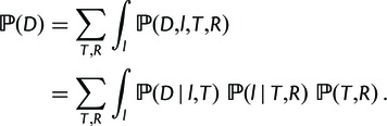
We considered real data from a well-studied system on yeast, for which the presence of a WGD was established based on synteny (Goffeau et al. 1996; Cliften et al. 2003; Kellis et al. 2003; Dietrich et al. 2004; Jones et al. 2004; Kellis et al. 2004; Braun et al. 2005; Byrne and Wolfe 2005; Van Het Hoog et al. 2007; Butler et al. 2009). Kellis et al. (2004) showed evidence of a WGD from synteny data by matching each syntenic region of Kluyveromyces waltii to two regions of Saccharomyces cerevisiae (i.e., 1:2 mapping) and inferred that “12% of the paralogous gene pairs were retained in each doubly conserved synteny block, and the remaining 88% of paralogous genes were lost” (Kellis et al. 2004, p. 621). We propose to check whether we also recover a retention rate around 12%, using our methods on a different set of data.
We used over 3,900 gene clusters identified by Butler et al. (2009) across 16 yeast species. To reflect their gene clustering method, we used a prior average of 1.05 genes at the root. Figure 6 shows the negative log-likelihood, profiled as a function of q. The reconciliation method, evaluated on a coarse grid of q values, infers a retention rate around 10% (0.1). The gene count method estimates it with more precision at 6.81% (0.0681) and within [0.058, 0.079] with 95% confidence. The observed LRT statistics was 9159.5 from the reconciliation method and 348.1 from the gene count method. Contrary to simulated data, empirical thresholds were not calculated due to the large size of the species tree. However, even if we conservatively choose the chi-square distribution with one degree of freedom to assess statistical significance, the threshold value is 7.88 at significance level 0.005, and both methods would return a P value well below  . Therefore, our methods provide extremely strong evidence for the presence of WGD in yeast, despite a low retention rate. The retention rate estimates were in general agreement between the two methods and with results from prior synteny-based research.
Fig. 6.

Profile of the negative log-likelihood from more than 3,900 gene families across 16 yeast species.
To assess the robustness of results to the prior at the root, we reestimated all parameters from gene counts using an average of two genes at the root a priori. Evidence for the WGD was still overwhelming (LRT statistic 309.4,  ) and the retention rate was not affected (0.0638).
Gene counts were used further to investigate the timing of the WGD. The likelihood was highest when the WGD was placed at time 0 from the most recent speciation on the branch, that is, just before the divergence between S. castellii and its sister clade. The log-likelihood profile led to a 95% confidence interval between 0 and 5.04 My prior to this divergence. These results are in agreement with prior work from Scannell et al. (2006, 2007), who found support for rapid diversification following the WGD. Placing the WGD just before the speciation did not affect the estimated retention rate (0.0690) or its 95% confidence interval [0.059, 0.080].
The reconciliation method was used to assess orthology, based on its estimation of each family’s reconciled gene tree. Figure 7 shows the estimated reconciled tree for family 1306, as an illustrative example. This reconciliation identifies two duplications and no loss at the WGD, and one duplication and ten losses at other locations in the species tree.
Fig. 7.

Estimated reconciled gene tree for family 1306, showing two duplications (filled circles) and no loss at the WGD, and one duplication (empty circle) and ten losses (crosses) elsewhere in the species tree.
Discussion
We propose here two new methods to test the presence and estimate the location of WGDs on a known species phylogeny. These methods use a set of gene families across multiple species, data now commonly built through clustering methods like orthoMCL (Li et al. 2003) from whole genomes or next-generation sequencing data. Contrary to synteny-based methods, our methods do not require positional information on the paralogs, are not sensitive to genome rearrangements, and can accommodate massive gene losses. Also, our gene count method is not affected by Ks saturation effects like Ks-based methods might be. Because our methods are based on an explicit WGD model, we can directly test the presence of WGDs. In contrast, methods relying on a mixture distribution of duplication times can be sensitive to the assumed ad hoc density of each component. For example, a mixture of several symmetric normal distributions might be needed to explain a single component from a skewed gamma distribution, therefore, making the estimated number of components rather uncertain. Our proposed methods thus appear complementary to other existing methods, which are based on different data types and different assumptions.
An advantage of our explicit model is that our methods can be extended to whole genome triplications, or more generally to k-fold instantaneous expansions followed by almost immediate loss of some replicate copies. Other explicit WGD models have been proposed by Hallinan and Lindberg (2011), who studied the distribution of chromosome counts in Mollusca, and by Maere et al. (2005) and Vanneste et al. (2013), who used an explicit model for the age of SSDs and duplications resulting from WGDs along a single lineage. Hallinan and Lindberg (2011) assume a background birth and death process for the evolution of the chromosome number along a known species tree, with the addition of a strict doubling at each WGD. Their probability model integrates over all possible number and placements of WGD events according to a Poisson distribution with constant rate δ (although restricted to no more than one WGD event on each branch). The absence of WGDs can then be tested by comparing the models with  versus
  . Because chromosome count data provide a single observation per lineage, WGDs are modeled with a random process and the method benefits from data across many species on a large tree. In contrast, our gene count method uses data from multiple independent gene families so that we can model each WGD specifically. Although our retention rate q accounts for some genes being almost immediately lost after a WGD, Hallinan and Lindberg (2011) can reasonably assume a strict doubling of the chromosome number (excluding partial genome duplications Freeling 2009).
Maere et al. (2005) and Vanneste et al. (2013) also proposed an explicit model for the number of gene paralogs with a certain age, to combine the effect of SSDs and that of large-scale duplications (WGD). Their model focuses on a single lineage and is mostly deterministic. The Ks distribution is modeled with an ad hoc Poisson smoothing to add randomness around the average ages of duplicates predicted from a population dynamics model. Their model considers separate SSD and WGD modes, with each duplicate evolving according to its own mode throughout the entire lineage. Gene losses are assumed to follow a power law decay with a different constant for each mode. Each gene copy thus “remembers” its initial duplication mode and disappears with the associated rate. This model allows for an elevated loss rate applying specifically to the genes created by the WGD. In contrast, our approach applies the same loss rate μ to all genes regardless of their origin, and a retention rate  is used instead to explain any elevated loss rate for a short period of time after a WGD.
Our model allows for incompletely sequenced genomes leading to incomplete gene families. This extension should be useful to include more species for analysis, to use data from expressed sequence tags (ESTs) or transcriptomes (as in Barker et al. 2008; Jiao et al. 2012; McKain et al. 2012). To account for incomplete genomes, our model assumes that genes from species u are sampled with frequency fu. These sampling frequencies are not estimated by our method but need to be determined separately, such as from transcriptome-sequencing depths. For instance, Lai et al. (2012, table 3) provide fu values for their data on compositae weeds, estimated from the percentage of ultraconserved orthologs (UCOs) recovered by their data assembly, among a benchmark database of 357 UCOs (Kozik et al. 2008). In their very recent work, Han et al. (2013) use a similar but richer model for incompletely sampled genomes and genomes with annotation error. Their error model could be used in conjunction with our WGD model.
We did not constrain the background duplication and loss rates  to be equal, as is done by Hallinan and Lindberg (2011, p.1153–1154, “static” and WGD models) or in computational analysis of gene family evolution (CAFE) (Hahn et al. 2005). We found that the constraint
  was necessary to stabilize estimation when the number of genes (or chromosomes) at the root is estimated or treated as a nuisance parameter (as was done in Hahn et al. [2005, 2007] and Hallinan and Lindberg [2011]). For instance, Hallinan and Lindberg (2011, fig. 3) showed a much wider confidence interval for the root count when λ and μ are allowed to differ, than when a single value
  is estimated. They also showed a positive estimate of
  from small root counts and a negative estimate of
  for large root counts (Hallinan and Lindberg 2011, table 1), pointing to a negative correlation between the estimate of the root count and the estimate of the net rate
  . Indeed, the same expected number of gene counts can be explained by a large count at the root and a large loss rate or by a small count at the root and a large duplication rate. Instead of attempting to estimate the number of genes at the root, our approach instead treats this count as a random variable with a geometric prior distribution. This strategy is showed to be successful at estimating both λ and μ separately in our simulation studies. Additionally, we found that calculating the likelihood conditional of the filtering procedure, including the fact that only nonextinct families can be observed, was very important to avoid biased estimates of λ and μ. The lack of conditioning strongly affected the estimated loss rate, which was underestimated to accommodate the unseen gene losses in the families that were filtered out. Proper conditioning restored unbiased estimates of λ and μ.
A limitation of our model is the assumption of constant rates λ and μ throughout the whole species tree. In contrast, Hahn et al. (2007) allow  to take different values on various branches of the species tree, to test hypotheses of heterogeneous rates among different lineages. Extra parameters could be considered in our model to allow for heterogeneity. For instance, a different loss rate μ could be allowed along a lineage following a WGD to test whether more extensive gene loss occurred following the WGD event. We expect our retention rate q to capture most of these extra gene losses, although not those occurring after the next speciation. This is a limitation if speciation follows rapidly after a WGD (Scannell et al. 2006, 2007) with the excess of losses extending after the speciation. Another limitation of our model is that all families are assumed to share the same rates λ, μ, and q. This is clearly an oversimplification. Hahn et al. (2005) showed that some gene families have undergone unusual expansions or contractions, for instance. Blanc and Wolfe (2004) showed that Arabidopsis gene families with regulatory functions have a higher retention rate at the most recent WGD event (α) than other functional categories. Independently, Seoighe and Gehring (2004) observed that genes involved in transcription regulation and signal transduction are more likely to be retained, and Maere et al. (2005) showed that genes involved in DNA metabolism, nuclease activity, and RNA binding are less likely to be retained. Our assumption that all gene lineages are retained independently at the WGD is another simplification. In particular, genes coding for subunits of the same protein complex would be expected to be lost together or retained together (gene balance hypothesis, e.g., Freeling 2009), and Konrad et al. (2011) showed evidence for loss rate variation depending on the gene age and functionalization.
Surprisingly, the gene count method provided more accurate rate estimates and more power to detect WGDs than the reconciliation method, despite its use of less information. We believe that this is due to the gene tree estimation and likelihood approximation used in the reconciliation method. Indeed, the exact likelihood of the gene count data is computationally tractable. The likelihood of the sequence data is much more challenging to obtain, however. Our reconciliation method computes an approximation by optimizing the gene tree for each family, with the assumption that the most important contributor to the likelihood is the most parsimonious reconciliation overall (as in Rasmussen and Kellis 2011), with its most parsimonious reconciliation at the WGD. In addition, optimization of the retention rate was based on a coarse grid due to the computational burden, which also prevented the estimation of λ and μ within the reconciliation method. We thus recommend the gene count method for the goal of estimating rates and testing the presence of WGDs. The reconciliation method is complementary for the purpose of estimating reconciled gene trees, where each duplication and loss is mapped to an edge in the species tree, and possibly to a WGD event. We leave it to future work to improve the reconciliation method and use an exact likelihood with a reduced computational burden, as this might provide more power to estimate the precise timing of WGD events.
Materials and Methods
Probabilistic Model
Model for WGDs and SSDs and Losses
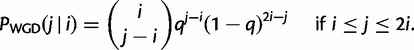
We assume that each gene family evolves according to a birth and death process (see Kendall 1949; Feller 1968) with birth rate λ for duplications and death rate μ for losses. Under this model, the probability that a family has j genes at time  given that it had i genes at time t0 only depends on the elapsed time t (Bailey 1964) and is given by
 |
where  is the probability that a single lineage goes extinct within time t:
 |
if  , and
, and  if
if  . The reconciliation method will only use the case i = 1, whereas the gene count method will need all
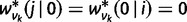
  values. We next consider a WGD at a fixed location in the species tree. At this WGD, each gene lineage is instantaneously duplicated, and the second copy is retained with probability q, or lost with probability
  . We assume independence between these events, that is, no interference between genes, both between and within families. Alternatively, our retention model can be described with a symmetric role for both gene copies, each being lost immediately with probability
  , but nonindependently to exclude the simultaneous loss of both copies. Before and after the WGD event (cf. fig. 8), gene lineages evolve according to the usual birth and death process. Each WGD event on the species tree is allowed to have its own retention rate q. The model and theory for whole genome triplications can be found in the supplementary material S1, Supplementary Material online.
Fig. 8.

Each WGD is represented by two extra nodes. The WGD model applies between these extra nodes (“at WGD”). The birth–death process applies to all other branches.
Number of Lineages at the Root
We introduce the use of a prior distribution to account for uncertainty in the ancestral gene number at the root of the species tree. Note that Hahn et al. (2005) treat the number of ancestral genes as a nuisance parameter, and Arvestad et al. (2009) and Rasmussen and Kellis (2011) assume one single gene at the root. We chose here a geometric prior distribution for the following reasons. First, there is no trivial stationary distribution for the birth and death process (other than 0 ancestral genes with probability 1). Then, a uniform prior might seem uninformative but it is not proper and contradicts our prior belief of only a few genes at the root. Using a geometric distribution with mean  , the prior probability for a ancestral genes at the root is
  for
for  . The choice
  corresponds to a mean of
  lineages at the root a priori. This is expected in the long run from the birth and death process under the condition that a unique lineage cannot be lost, and if
  . This last condition is restrictive, however, so we leave the choice of η unconstrained. All a lineages present at the root might not be observed in the gene tree as some may go extinct. The geometric distribution enables a closed-form probability of s surviving lineages observed at the root of the reconciled tree (Csűrös and Miklós 2009, Corollary 9):
 |
(1) |
where  and
and  is the probability that a lineage starting at the root of the species tree is “doomed” with no descendants in any of the species (see next section). The reconciliation method will further need the probability that s lineages survive and give rise to subtrees
  with reconciliations
  , which is given by
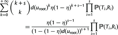 |
where  is the probability of observing the reconciled subtree
  given a single gene at the root (see below).
Conditioning on the Data Collection Process
The likelihood of an observed gene family i is the conditional probability of the data Di for that family, conditional on the family being actually observed and not filtered out of the data set. If no specific filtering is applied, this is
 |
Using our geometric prior distribution at the root, the probability that a gene family goes completely extinct (and thus unobserved) is:
 |
(2) |
where  is the root of the species tree, and d(v) is the probability that a single lineage starting at node v is doomed with no descendants in any species below v. These probabilities can be computed with a postorder traversal of the species tree (e.g., Csűrös and Miklós 2006; Rasmussen and Kellis 2011). Indeed, if v has children vk at distances tk with the birth–death process applying along the edges between v and vk, then
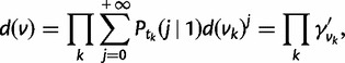 |
(3) |
where  . For each WGD, two nodes are added in the species tree:
  just before the WGD and
  just after the WGD, each with a single child (fig. 8). The birth and death process applies along each edge in the species tree, except between
  and
and  where the WGD model applies instead. Therefore,
  can be computed from equation (3). To determine
  , we note that a lineage entering the WGD at
  is doomed either if both copies from the WGD are retained and later doomed, or if the second copy is lost and the first copy is doomed. Therefore
If the filtering process consists of keeping families with at least one gene in each of the left and the right subclades descending from the root, then the correct likelihood of data Di for family i is 
 with
with
| (4) |
where  and
and  are the probabilities that a family leaves no descendants in the right (or left) subclade. They can be calculated using the doom probabilities within each specific subclade, that is, using (2) with
  replaced by
 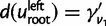 or
or 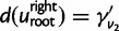 , the two factors of (3) at
  .
.
Incompletely Sampled Genomes
To relax the assumption of completely sequenced genomes, we allow for some genes to be unsampled in some species. To do so, we assume that each gene in species u has probability fu to be sampled, independently of other genes. For a species u with a complete genome sequence, fu is just 1. For species whose data originate from ESTs or transcriptomes,  , and could be rather low at low sequencing depths. This sampling step is accommodated by an extra node along each external edge of the species tree, located at distance 0 of each tip (species). Between this node and species u, each gene lineage is either retained with probability fu or lost with probability
  . Instead of applying the birth–death transition probabilities
  along these new branches, we apply the following binomial probabilities of sampling j genes from species u given that i genes are truly present:
 |
In the context of speciation models, the same sampling was used by FitzJohn et al. (2009), where this step is equivalent to a mass extinction event.
Statistical Test for the Presence of a WGD
Let Di denote the data for family i, for  families total. The reconciliation method will use the sequence alignment as data Di, while the gene count method will use gene counts only. Recall first that likelihoods are calculated as conditional probabilities. More specifically, the likelihood of family i given a particular species tree (with potential WGDs) is
  , where
  is described below and
  does not depend on i but depends on the particular filtering step (as described earlier).
Let 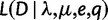 be the likelihood of the full data
  given a species tree with a WGD placed on edge e with retention rate q. Assuming that gene families are independent, this is simply the product
 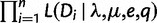 , where each term is the likelihood of a single family. These likelihoods are calculated at fixed, supposedly known values of λ and μ for the reconciliation method, given the computational burden. In contrast, we can use the profile likelihood when using gene counts, to optimize λ and μ at each retention rate:
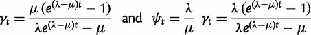
To test the presence of a WGD on edge e, the LRT uses
because the absence of WGD corresponds to q = 0. When the WGD is hypothesized to be placed on either of several branches in the species tree, one  is calculated for each edge e where the WGD might occur. The placement of the WGD is then estimated to be the edge e that maximizes
  . To test the presence of a WGD along any of these edges, the LRT uses the maximum
  value over all hypothesized edges e.
Because the absence of WGD corresponds to the boundary q = 0 of the parameter space  , we do not expect
  to have a chi-square distribution under the null hypothesis. Under regularity assumptions (Self and Liang 1987), the asymptotic distribution of such a LRT statistic is a 50:50 mixture of a point mass at q = 0 and a chi-square distribution with 1 degree of freedom. This distribution was used to determine P values for the gene count method. Accordingly, the threshold to reject the absence of WGD is
  at significance level
  , or
, or  for
for  , or
, or  at level
  . The profile likelihood
  from gene counts was used to determine a 95% confidence interval for q, obtained as the set of all values such that
  (Venzon and Moolgavkar 1988).
The reconciliation method was too slow to allow a thorough optimization of q in [0,1]. The likelihood was instead maximized over the grid 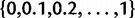 , and the estimate of q was the value on this grid that maximized the likelihood. Because of this discretization and of the likelihood approximation for the reconciliation method, we used an empirical threshold for detecting the presence of a WGD with the reconciliation method. This threshold was the value c such that no more than 5% of data sets simulated under no WGD had
  .
.
Probabilities for the Reconciliation Method
The reconciliation method uses the likelihood of sequence alignments. To ease notations, D will denote here the sequence alignment of a single gene family. Its probability is obtained by integrating out the unobserved gene tree topology T, its reconciliation R with the species tree, and the gene tree branch lengths l:
 |
(5) |
The Hasegawa–Kishino–Yano model (HKY, Hasegawa et al. 1985) is used for the probability of the sequence alignment given the gene tree,  . To relax the clock assumption on gene trees, we follow Rasmussen and Kellis (2011) to model branch lengths in gene trees and to get
  (setting branch lengths to 0 along any WGD edge). Each family has its own rate (so-called gene-specific rate) and each branch of the species tree also has its own specific rate (Rasmussen and Kellis 2007, p.277 for full details). Finally, the probability
  of a gene tree and its reconciliation given the species tree is calculated according to our birth–death and WGD model, and described in more detail below.
Dealing with all possible reconciliations is very challenging (Arvestad et al. 2009), so here we approximate (5) by the maximum quantity inside the sum, that is by  where
where  ,
,  , and
, and  are the maximum a posteriori estimators of l, T, and R given the data. Moreover, for each gene topology T, we only consider its most parsimonious reconciliation R as in Rasmussen and Kellis (2011). In the presence of WGDs, we further restrict our search to the most parsimonious reconciliation of the gene subtree along each branch with a WGD, to maximize the number of duplications at the WGD and then minimize the number of losses at the WGD. We provide a fast algorithm to compute this most parsimonious reconciliation along a branch with a WGD (supplementary material S1, Supplementary Material online). This approximation is expected to perform well when λ and μ are small and when q is large (for branches with WGDs).
To calculate the reconciled topology prior probability  given a species tree with potential WGDs, we use the fast algorithm in Arvestad et al. (2003, 2009) and Rasmussen and Kellis (2011). This algorithm uses a postorder tree traversal because
  can be factorized into the probability of gene subtrees within each branch in the species tree, as explained in Rasmussen and Kellis (2011). In their equation (13), the only terms that need to be adapted for the presence of WGDs are the probabilities
  , for a node u in the species tree, a speciation node ν in the gene tree reconciled to the parent of u, and the gene subtree
  rooted at ν with its descendant nodes reconciled at u. If the birth–death process applies to the parent edge of u, of length t, then
 where k is the number of leaves in subtree
  ,
,  and f is a factor depending on the topology and labels of
  (Rasmussen and Kellis 2011, eq. 13c). Within WGD edges, that is, when
  for some WGD, the WGD model applies instead of the birth–death process. In this case, the reconciled subtree
  starts with a single lineage ν entering node
  . The only options are
  or
or  , where T1 has a single tip (k = 1 gene copy survives after the WGD) and T2 has k = 2 tips (both gene copies are retained and survive after the WGD). The probability
  is then still given by
 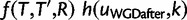 , where
  is unchanged. The new term
  is simply q for k = 2 and
 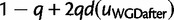 for k = 1, to account for the possibility that both copies are retained at the WGD but one is doomed.
Probabilities for the Gene Count Method
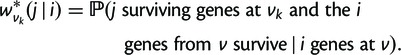
In this section, D denotes the gene count data for a single family. Its probability can be obtained using a postorder tree traversal as in CAFE (De Bie et al. 2006), also called probabilistic graphical model in Hahn et al. (2005). From the tips to the root, we calculate at each node v in the species tree the probabilities of observing the data Dv in the descendants of v conditional on i surviving gene lineages at v, with the algorithm by Csűrös and Miklós (2009). In this algorithm, the key component that needs to be extended to WGDs is the survival transition probability
 |
Along an edge with the birth–death process, Csűrös and Miklós (2009) showed how to efficiently calculate all the necessary  values recursively using
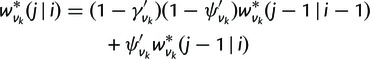 |
and initial conditions 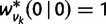 ,
,  for
for  , where
  is as in equation (3) and
 . Along an edge with a WGD, the birth–death transition probability
  is replaced by the probability that i genes before the WGD give rise to j genes immediately after the WGD. This is derived from a binomial distribution:
 |
The survival transition probabilities along the WGD edge into  are obtained by
  ,
,  ,
, 
 and the recursion formula
 |
The probabilities  are initialized at each tip v as 1 if species v has i genes and as 0 for other values of i (or 1 for all i if v has missing data). Once these probabilities are calculated at the root
  , the probability of the full data is obtained using the shifted geometric prior for the ancestral surviving count:
 with
with  from equation (1).
Simulation Study
We used the four-taxon species tree in figure 9 to evaluate the performance of both methods. The depth of the species tree was set to 18.03 My (from Butler et al. [2009]), with background rates of  and
and  events per million year. Under no WGD, these values lead to 38% of families with at most one gene in each species. A WGD was placed on the middle of the branch ancestral to taxa A and B. The SPIMAP simulation tool was adapted to include WGDs and used to simulate gene trees either with or without a WGD, starting from a single gene lineage at the root. The true retention rate at the WGD varied from low to high:
  , 0.5, or
  . SPIMAP estimates gene trees for families of three or more genes, so families with fewer genes were filtered out when applying the reconciliation method. Families with only one gene were filtered out for the gene count method. For each retention rate, we generated 20,000 families for the reconciliation method and 1 million families for the gene count method (after filtering). To generate branch-specific rates on the species tree, we used the gamma distribution with parameters
  and
and  . Gene-specific rates were generated from the inverse gamma distribution with parameters
  and
and  (with a mean of 1). These values were estimated from real data in Rasmussen and Kellis (2011) and correspond to an average of 0.0765 substitutions per site from the root to tip D for instance. Gene tree branch lengths were then calculated under the model in Rasmussen and Kellis (2011), from which 500 bp sequences were simulated under the Jukes–Cantor model (Felsenstein 2004).
For analysis, both methods were used with a geometric prior for the number of gene lineages at the root, with a mean of 2 ( ). For the reconciliation method, instead of conditioning on each family having at least three genes, we only conditioned on observing some data (one or more genes). Indeed, obtaining a theoretical formula for this actual filtering step is quite challenging. The gene count method used a conditional likelihood to reflect that retained families had at least two genes. The data were first analyzed assuming the correct location of the WGD, then analyzed again assuming an uncertain placement of the putative WGD: either at its true location or at the middle of the parental edge, ancestral to species A, B, and C (fig. 9).
For the gene count method, for each retention rate, the simulated gene families were grouped into 100 independent sets of either n = 500, 1,000, or 5,000 families each, and into 50 independent sets of  families each. The duplication/loss and retention rates
  were jointly estimated from each set.
The reconciliation method being much more computationally heavy, we used a resampling procedure to evaluate its performance. For each targeted number of gene families from n = 500 to 5,000, we randomized the order of the 20,000 families, then combined consecutive families to form 20,000/ sets of n families. This was repeated
  times to obtain a total of 10,000 sets of n families. To obtain 10,000 sets of
  gene families each, we resampled the originally simulated 20,000 families with replacement. The advantage of this procedure is that it only required the initial analysis of each of the 20,000 simulated families individually 11 times, assuming q in
  . Each analysis used 20,000 iterations in SPIMAP and the true values of
  and
and  . These individual family results were later used for the grid-based optimization of q from each set. A grid search strategy allowed us to use parallel computing resources efficiently to distribute jobs across many simulation replicates, but more powerful algorithms (like the golden section search) could be used in other situations.
Analysis of the Yeast Data
The sequence data for the 9,209 gene families identified by Butler et al. (2009) were downloaded from http://compbio.mit.edu/candida (last accessed January 1, 2014). The 16-species yeast tree was also taken from this recent study. The hypothesized WGD was placed on its known location, along the branch ancestral to the clade containing S. castellii and S. cerevisiae, arbitrarily in the middle of that branch (see fig. 10). From the 9,209 original gene families, only 3,932 families had at least one gene in each subclade stemming from the root (the Candida subclade and the Saccharomyces subclade). Because our WGD model does not allow for de novo genes, the data set was reduced to these 3,932 families. All of them were used for the gene count method. For the reconciliation method, we could only include gene families with three or more genes, which reduced the data set further to 3,909 families. For both methods, the likelihoods were conditional of families having at least one gene in each of the two major subclades.
Fig. 10.

Phylogeny of 16 yeast species from Butler et al. (2009).
To model uncertainty at the root, we use  to fix a low number of ancestral genes at the root a priori (1.05) but still allow for some families to have more than one gene lineage at the root. This was necessary because the method used by Butler et al. (2009) to build gene clusters used an iterative method to divide any large cluster with two or more reconstructed genes at the root into separate gene clusters.
The gene count method jointly estimated all rates  by maximum likelihood. The profile log-likelihood of the gene count data was also calculated by fixing q and maximizing the likelihood over the other parameters
  only, and then used to get a 95% confidence interval for q. For the reconciliation method, SPIMAP (with WGD implementation) used the duplication/loss rates obtained from the gene count method based on the null hypothesis of no WGD (
 and
and  ). To limit computation time, SPIMAP was run for 20,000 iterations for small families up to 40 genes, for 8,000 iterations for families with 41–56 genes, and for 5,000 iterations for larger families. For the species-specific and gene-specific rate distributions, we used the values estimated by Rasmussen and Kellis (2011), which were based on 739 one-to-one orthologous families.
Gene counts were used for further analyses to investigate the timing of the WGD, which was optimized along with λ, μ, and q using maximum likelihood.
Supplementary Material
Supplementary material S1 is available at Molecular Biology and Evolution online (http://www.mbe.oxfordjournals.org/)
Acknowledgments
This work was supported in part by the National Science Foundation (DEB 0949121). We thank Matthew Rasmussen for help with SPIMAP and two anonymous reviewers for their very constructive comments. The simulations were performed using computing assistance from Bill Taylor and Mike Cammilleri, and resources of the UW-Madison Center for High Throughput Computing (CHTC) in the Department of Computer Sciences. The CHTC is supported by UW-Madison and the Wisconsin Alumni Research Foundation, and is an active member of the Open Science Grid, which is supported by the National Science Foundation and the U.S. Department of Energy’s Office of Science.
References
- Amores A, Force A, Yan YL, Joly L, Amemiya C, Fritz A, Ho RK, Langeland J, Prince V, Wang YL, et al. Zebrafish hox clusters and vertebrate genome evolution. Science. 1998;282:1711–1714. doi: 10.1126/science.282.5394.1711. [DOI] [PubMed] [Google Scholar]
- Arvestad L, Berglund A, Lagergren J, Sennblad B. Bayesian gene/species tree reconciliation and orthology analysis using MCMC. Bioinformatics. 2003;19:i7–i15. doi: 10.1093/bioinformatics/btg1000. [DOI] [PubMed] [Google Scholar]
- Arvestad L, Lagergren J, Sennblad B. The gene evolution model and computing its associated probabilities. J ACM. 2009;56:1–44. [Google Scholar]
- Bailey N. The elements of stochastic processes. New York: Wiley; 1964. [Google Scholar]
- Barker MS, Kane NC, Matvienko M, Kozik A, Michelmore RW, Knapp SJ, Rieseberg LH. Multiple paleopolyploidizations during the evolution of the compositae reveal parallel patterns of duplicate gene retention after millions of years. Mol Biol Evol. 2008;25:2445–2455. doi: 10.1093/molbev/msn187. [DOI] [PMC free article] [PubMed] [Google Scholar]
- Barker MS, Vogel H, Schranz ME. Paleopolyploidy in the Brassicales: analyses of the Cleome transcriptome elucidate the history of genome duplications in Arabidopsis and other Brassicales. Genome Biol Evol. 2009;1:391–399. doi: 10.1093/gbe/evp040. [DOI] [PMC free article] [PubMed] [Google Scholar]
- Blanc G, Wolfe KH. Widespread paleopolyploidy in model plant species inferred from age distributions of duplicate genes. Plant Cell. 2004;16:1667–1678. doi: 10.1105/tpc.021345. [DOI] [PMC free article] [PubMed] [Google Scholar]
- Bowers JE, Chapman BA, Rong J, Paterson AH. Unravelling angiosperm genome evolution by phylogenetic analysis of chromosomal duplication events. Nature. 2003;422:433–438. doi: 10.1038/nature01521. [DOI] [PubMed] [Google Scholar]
- Braun BR, Van Het Hoog M, d’Enfert C, Martchenko M, Dungan J, Kuo A, Inglis DO, Uhl MA, Hogues H, Berriman M, et al. A human-curated annotation of the Candida albicans genome. PLoS Genet. 2005;1:e1. doi: 10.1371/journal.pgen.0010001. [DOI] [PMC free article] [PubMed] [Google Scholar]
- Butler G, Rasmussen M, Lin M, Santos MA, Sakthikumar S, Munro CA, Rheinbay E, Grabherr M, Forche A, Reedy JL, et al. Evolution of pathogenicity and sexual reproduction in eight Candida genomes. Nature. 2009;459:657–662. doi: 10.1038/nature08064. [DOI] [PMC free article] [PubMed] [Google Scholar]
- Byrne KP, Wolfe KH. The yeast gene order browser: combining curated homology and syntenic context reveals gene fate in polyploid species. Genome Res. 2005;15:1456–1461. doi: 10.1101/gr.3672305. [DOI] [PMC free article] [PubMed] [Google Scholar]
- Cliften P, Sudarsanam P, Desikan A, Fulton L, Fulton B, Majors J, Waterston R, Cohen BA, Johnston M. Finding functional features in saccharomyces genomes by phylogenetic footprinting. Science. 2003;301:71–76. doi: 10.1126/science.1084337. [DOI] [PubMed] [Google Scholar]
- Csűrös M, Miklós I. A probabilistic model for gene content evolution with duplication, loss, and horizontal transfer. In: Apostolico A, Guerra C, Istrail S, Pevzner P, Waterman M, editors. Research in computational molecular biology. Vol. 3909, Lecture notes in computer science. Berlin: Springer; 2006. pp. 206–220. [Google Scholar]
- Csűrös M, Miklós I. Streamlining and large ancestral genomes in archaea inferred with a phylogenetic birth-and-death model. Mol Biol Evol. 2009;26:2087–2095. doi: 10.1093/molbev/msp123. [DOI] [PMC free article] [PubMed] [Google Scholar]
- Cui L, Wall PK, Leebens-Mack JH, Lindsay BG, Soltis DE, Doyle JJ, Soltis PS, Carlson JE, Arumuganathan K, Barakat A, et al. Widespread genome duplications throughout the history of flowering plants. Genome Res. 2006;16:738–749. doi: 10.1101/gr.4825606. [DOI] [PMC free article] [PubMed] [Google Scholar]
- D’Hont A, Denoeud F, Aury J, Baurens FC, Carreel F, Garsmeur O, Noel B, Bocs S, Droc G, Rouard M, et al. The banana (Musa acuminata) genome and the evolution of monocotyledonous plants. Nature. 2012;488:213–217. doi: 10.1038/nature11241. [DOI] [PubMed] [Google Scholar]
- De Bie T, Cristianini N, Demuth J, Hahn M. Cafe: a computational tool for the study of gene family evolution. Bioinformatics. 2006;22:1269–1271. doi: 10.1093/bioinformatics/btl097. [DOI] [PubMed] [Google Scholar]
- Dehal P, Boore JL. Two rounds of whole genome duplication in the ancestral vertebrate. PLoS Biol. 2005;3:e314. doi: 10.1371/journal.pbio.0030314. [DOI] [PMC free article] [PubMed] [Google Scholar]
- Dietrich FS, Voegeli S, Brachat S, Lerch A, Gates K, Steiner S, Mohr C, Pöhlmann R, Luedi P, Choi S, et al. The Ashbya gossypii genome as a tool for mapping the ancient Saccharomyces cerevisiae genome. Science. 2004;304:304–307. doi: 10.1126/science.1095781. [DOI] [PubMed] [Google Scholar]
- Feller W. An introduction to probability theory and its applications. New York: Wiley; 1968. [Google Scholar]
- Felsenstein J. Inferring phylogenies. Sunderland (MA): Sinauer Associates; 2004. [Google Scholar]
- FitzJohn RG, Maddison WP, Otto SP. Estimating trait-dependent speciation and extinction rates from incompletely resolved phylogenies. Syst Biol. 2009;58:595–611. doi: 10.1093/sysbio/syp067. [DOI] [PubMed] [Google Scholar]
- Freeling M. Bias in plant gene content following different sorts of duplication: tandem, whole-genome, segmental, or by transposition. Annu Rev Plant Biol. 2009;60:433–453. doi: 10.1146/annurev.arplant.043008.092122. [DOI] [PubMed] [Google Scholar]
- Gernhard T. The conditioned reconstructed process. J Theor Biol. 2008;253:769–778. doi: 10.1016/j.jtbi.2008.04.005. [DOI] [PubMed] [Google Scholar]
- Goffeau A, Barrell B, Bussey H, Davis RW, Dujon B, Feldmann H, Galibert F, Hoheisel JD, Jacq C, Johnston M, et al. Life with 6000 genes. Science. 1996;274:546–567. doi: 10.1126/science.274.5287.546. [DOI] [PubMed] [Google Scholar]
- Grant D, Cregan P, Shoemaker RC. Genome organization in dicots: genome duplication in Arabidopsis and synteny between soybean and Arabidopsis. Proc Natl Acad Sci U S A. 2000;97:4168–4173. doi: 10.1073/pnas.070430597. [DOI] [PMC free article] [PubMed] [Google Scholar]
- Hahn M, De Bie T, Stajich J, Nguyen C, Cristianini N. Estimating the tempo and mode of gene family evolution from comparative genomic data. Genome Res. 2005;15:1153–1160. doi: 10.1101/gr.3567505. [DOI] [PMC free article] [PubMed] [Google Scholar]
- Hahn M, Demuth J, Han S. Accelerated rate of gene gain and loss in primates. Genetics. 2007;177:1941–1949. doi: 10.1534/genetics.107.080077. [DOI] [PMC free article] [PubMed] [Google Scholar]
- Hallinan N, Lindberg D. Comparative analysis of chromosome counts infers three paleopolyploidies in the mollusca. Genome Biol Evol. 2011;3:1150–1163. doi: 10.1093/gbe/evr087. [DOI] [PMC free article] [PubMed] [Google Scholar]
- Han MV, Thomas GW, Lugo-Martinez J, Hahn MW. Estimating gene gain and loss rates in the presence of error in genome assembly and annotation using cafe 3. Mol Biol Evol. 2013;30:1987–1997. doi: 10.1093/molbev/mst100. [DOI] [PubMed] [Google Scholar]
- Hasegawa M, Kishino H, Yano T. Dating of the human-ape splitting by a molecular clock of mitochondrial DNA. J Mol Evol. 1985;22:160–174. doi: 10.1007/BF02101694. [DOI] [PubMed] [Google Scholar]
- Jackson AP. Evolutionary consequences of a large duplication event in Trypanosoma brucei: chromosomes 4 and 8 are partial duplicons. BMC Genomics. 2007;8:432. doi: 10.1186/1471-2164-8-432. [DOI] [PMC free article] [PubMed] [Google Scholar]
- Jaillon O, Aury JM, Noel B, Policriti A, Clepet C, Casagrande A, Choisne N, Aubourg S, Vitulo N, Jubin C, et al. The grapevine genome sequence suggests ancestral hexaploidization in major angiosperm phyla. Nature. 2007;449:463–467. doi: 10.1038/nature06148. [DOI] [PubMed] [Google Scholar]
- Jiao Y, Leebens-Mack J, Ayyampalayam S, Bowers JE, McKain MR, McNeal J, Rolf M, Ruzicka DR, Wafula E, Wickett NJ, et al. A genome triplication associated with early diversification of the core eudicots. Genome Biol. 2012;13:R3. doi: 10.1186/gb-2012-13-1-r3. [DOI] [PMC free article] [PubMed] [Google Scholar]
- Jiao Y, Wickett N, Ayyampalayam S, Chanderbali AS, Landherr L, Ralph PE, Tomsho LP, Hu Y, Liang H, Soltis PS, et al. Ancestral polyploidy in seed plants and angiosperms. Nature. 2011;473:97–100. doi: 10.1038/nature09916. [DOI] [PubMed] [Google Scholar]
- Jones T, Federspiel NA, Chibana H, Dungan J, Kalman S, Magee BB, Newport G, Thorstenson YR, Agabian N, Magee PT, et al. The diploid genome sequence of Candida albicans. Proc Natl Acad Sci U S A. 2004;101:7329–7334. doi: 10.1073/pnas.0401648101. [DOI] [PMC free article] [PubMed] [Google Scholar]
- Kellis M, Birren B, Lander E. Proof and evolutionary analysis of ancient genome duplication in the yeast Saccharomyces cerevisiae. Nature. 2004;428:617–624. doi: 10.1038/nature02424. [DOI] [PubMed] [Google Scholar]
- Kellis M, Patterson N, Endrizzi M, Birren B, Lander E. Sequencing and comparison of yeast species to identify genes and regulatory elements. Nature. 2003;423:241–254. doi: 10.1038/nature01644. [DOI] [PubMed] [Google Scholar]
- Kendall D. Stochastic processes and population growth. J R Stat Soc B. 1949;11:230–282. [Google Scholar]
- Konrad A, Teufel AI, Grahnen JA, Liberles DA. Toward a general model for the evolutionary dynamics of gene duplicates. Genome Biol Evol. 2011;3:1197–1209. doi: 10.1093/gbe/evr093. [DOI] [PMC free article] [PubMed] [Google Scholar]
- Kozik A, Matvienko M, Kozik I, Van Leeuwen H, Van Deynze A, Michelmore R. Plant and animal genomes conference. 2008. Eukaryotic ultra conserved orthologs and estimation of gene capture in EST libraries. In: San Diego, CA. Vol. 16. p P6. [Google Scholar]
- Ku HM, Vision T, Liu J, Tanksley SD. Comparing sequenced segments of the tomato and Arabidopsis genomes: large-scale duplication followed by selective gene loss creates a network of synteny. Proc Natl Acad Sci U S A. 2000;97:9121–9126. doi: 10.1073/pnas.160271297. [DOI] [PMC free article] [PubMed] [Google Scholar]
- Lai Z, Kane NC, Kozik A, Hodgins KA, Dlugosch KM, Barker MS, Matvienko M, Yu Q, Turner KG, Pearl SA, et al. Genomics of compositae weeds: EST libraries, microarrays, and evidence of introgression. Am J Bot. 2012;99:209–218. doi: 10.3732/ajb.1100313. [DOI] [PubMed] [Google Scholar]
- Langham RJ, Walsh J, Dunn M, Ko C, Goff SA, Freeling M. Genomic duplication, fractionation and the origin of regulatory novelty. Genetics. 2004;166:935–945. doi: 10.1534/genetics.166.2.935. [DOI] [PMC free article] [PubMed] [Google Scholar]
- Leitch I, Bennett M. Genome downsizing in polyploid plants. Biol J Linn Soc. 2004;82:651–663. [Google Scholar]
- Li L, Stoeckert CJ, Roos DS. OrthoMCL: identification of ortholog groups for eukaryotic genomes. Genome Res. 2003;13:2178–2189. doi: 10.1101/gr.1224503. [DOI] [PMC free article] [PubMed] [Google Scholar]
- Lynch M, Conery JS. The evolutionary fate and consequences of duplicate genes. Science. 2000;290:1151–1155. doi: 10.1126/science.290.5494.1151. [DOI] [PubMed] [Google Scholar]
- Lyons E, Pedersen B, Kane J, Alam M, Ming R, Tang H, Wang X, Bowers J, Paterson A, Lisch D, et al. Finding and comparing syntenic regions among Arabidopsis and the outgroups papaya, poplar, and grape: coge with rosids. Plant Physiol. 2008;148:1772–1781. doi: 10.1104/pp.108.124867. [DOI] [PMC free article] [PubMed] [Google Scholar]
- Maere S, De Bodt S, Raes J, Casneuf T, Van Montagu M, Kuiper M, Van de Peer Y. Modeling gene and genome duplications in eukaryotes. Proc Natl Acad Sci U S A. 2005;102:5454–5459. doi: 10.1073/pnas.0501102102. [DOI] [PMC free article] [PubMed] [Google Scholar]
- Mayer K, Murphy G, Tarchini R, Wambutt R, Volckaert G, Pohl T, Düsterhöft A, Stiekema W, Entian KD, Terryn N, et al. Conservation of microstructure between a sequenced region of the genome of rice and multiple segments of the genome of Arabidopsis thaliana. Genome Res. 2001;11:1167–1174. doi: 10.1101/gr.161701. [DOI] [PMC free article] [PubMed] [Google Scholar]
- McKain MR, Wickett N, Zhang Y, Ayyampalayam S, McCombie WR, Chase MW, Pires JC, dePamphilis CW, Leebens-Mack J. Phylogenomic analysis of transcriptome data elucidates co-occurrence of a paleopolyploid event and the origin of bimodal karyotypes in agavoideae (asparagaceae) Am J Bot. 2012;99:397–406. doi: 10.3732/ajb.1100537. [DOI] [PubMed] [Google Scholar]
- Opazo JC, Butts GT, Nery MF, Storz JF, Hoffmann FG. Whole-genome duplication and the functional diversification of teleost fish hemoglobins. Mol Biol Evol. 2013;30:140–153. doi: 10.1093/molbev/mss212. [DOI] [PMC free article] [PubMed] [Google Scholar]
- Panopoulou G, Poustka AJ. Timing and mechanism of ancient vertebrate genome duplications—the adventure of a hypothesis. Trends Genet. 2005;21:559–567. doi: 10.1016/j.tig.2005.08.004. [DOI] [PubMed] [Google Scholar]
- Paterson AH, Bowers JE, Burow MD, Draye X, Elsik CG, Jiang CX, Katsar CS, Lan TH, Lin YR, Ming R, et al. Comparative genomics of plant chromosomes. Plant Cell. 2000;12:1523–1539. doi: 10.1105/tpc.12.9.1523. [DOI] [PMC free article] [PubMed] [Google Scholar]
- Putnam NH, Butts T, Ferrier DE, Furlong RF, Hellsten U, Kawashima T, Robinson-Rechavi M, Shoguchi E, Terry A, Yu JK, et al. The amphioxus genome and the evolution of the chordate karyotype. Nature. 2008;453:1064–1071. doi: 10.1038/nature06967. [DOI] [PubMed] [Google Scholar]
- Rasmussen M, Kellis M. Accurate gene-tree reconstruction by learning gene-and species-specific substitution rates across multiple complete genomes. Genome Res. 2007;17:1932–1942. doi: 10.1101/gr.7105007. [DOI] [PMC free article] [PubMed] [Google Scholar]
- Rasmussen M, Kellis M. A Bayesian approach for fast and accurate gene tree reconstruction. Mol Biol Evol. 2011;28:273–290. doi: 10.1093/molbev/msq189. [DOI] [PMC free article] [PubMed] [Google Scholar]
- Scannell DR, Byrne KP, Gordon JL, Wong S, Wolfe KH. Multiple rounds of speciation associated with reciprocal gene loss in polyploid yeasts. Nature. 2006;440:341–345. doi: 10.1038/nature04562. [DOI] [PubMed] [Google Scholar]
- Scannell DR, Frank AC, Conant GC, Byrne KP, Woolfit M, Wolfe KH. Independent sorting-out of thousands of duplicated gene pairs in two yeast species descended from a whole-genome duplication. Proc Natl Acad Sci U S A. 2007;104:8397–8402. doi: 10.1073/pnas.0608218104. [DOI] [PMC free article] [PubMed] [Google Scholar]
- Schlueter JA, Dixon P, Granger C, Grant D, Clark L, Doyle JJ, Shoemaker RC. Mining EST databases to resolve evolutionary events in major crop species. Genome. 2004;47:868–876. doi: 10.1139/g04-047. [DOI] [PubMed] [Google Scholar]
- Self SG, Liang KY. Asymptotic properties of maximum likelihood estimators and likelihood ratio tests under nonstandard conditions. J Am Stat Assoc. 1987;82:605–610. [Google Scholar]
- Seoighe C, Gehring C. Genome duplication led to highly selective expansion of the Arabidopsis thaliana proteome. Trends Genet. 2004;20:461–464. doi: 10.1016/j.tig.2004.07.008. [DOI] [PubMed] [Google Scholar]
- Song K, Lu P, Tang K, Osborn TC. Rapid genome change in synthetic polyploids of Brassica and its implications for polyploid evolution. Proc Natl Acad Sci U S A. 1995;92:7719–7723. doi: 10.1073/pnas.92.17.7719. [DOI] [PMC free article] [PubMed] [Google Scholar]
- Tang H, Bowers JE, Wang X, Ming R, Alam M, Paterson AH. Synteny and collinearity in plant genomes. Science. 2008;320:486–488. doi: 10.1126/science.1153917. [DOI] [PubMed] [Google Scholar]
- Taylor JS, Braasch I, Frickey T, Meyer A, Van de Peer Y. Genome duplication, a trait shared by 22,000 species of ray-finned fish. Genome Res. 2003;13:382–390. doi: 10.1101/gr.640303. [DOI] [PMC free article] [PubMed] [Google Scholar]
- Tomato Genome Consortium. The tomato genome sequence provides insights into fleshy fruit evolution. Nature. 2012;485:635–641. doi: 10.1038/nature11119. [DOI] [PMC free article] [PubMed] [Google Scholar]
- Van de Peer Y, Taylor JS, Meyer A. Are all fishes ancient polyploids? Netherlands: Springer; 2003. [PubMed] [Google Scholar]
- Van Het Hoog M, Rast TJ, Martchenko M, Grindle S, Dignard D, Hogues H, Cuomo C, Berriman M, Scherer S, Magee BB, et al. Assembly of the Candida albicans genome into sixteen supercontigs aligned on the eight chromosomes. Genome Biol. 2007;8:R52. doi: 10.1186/gb-2007-8-4-r52. [DOI] [PMC free article] [PubMed] [Google Scholar]
- Vanneste K, Van de Peer Y, Maere S. Inference of genome duplications from age distributions revisited. Mol Biol Evol. 2013;30:177–190. doi: 10.1093/molbev/mss214. [DOI] [PubMed] [Google Scholar]
- Venzon D, Moolgavkar S. A method for computing profile-likelihood-based confidence intervals. J R Stat Soc C. 1988;37:87–94. [Google Scholar]
- Vision TJ, Brown DG, Tanksley SD. The origins of genomic duplications in Arabidopsis. Science. 2000;290:2114–2117. doi: 10.1126/science.290.5499.2114. [DOI] [PubMed] [Google Scholar]
- Wolfe KH, Shields DC. Molecular evidence for an ancient duplication of the entire yeast genome. Nature. 1997;387:708–712. doi: 10.1038/42711. [DOI] [PubMed] [Google Scholar]
Associated Data
This section collects any data citations, data availability statements, or supplementary materials included in this article.