A Flexible Two-Dimensional Mortality Model for Use in Indirect Estimation

Abstract

Mortality estimates for many populations are derived using model life tables, which describe typical age patterns of human mortality. We propose a new system of model life tables as a means of improving the quality and transparency of such estimates. A flexible two-dimensional model was fitted to a collection of life tables from the Human Mortality Database. The model can be used to estimate full life tables given one or two pieces of information: child mortality only, or child and adult mortality. Using life tables from a variety of sources, we have compared the performance of new and old methods. The new model outperforms the Coale-Demeny and UN model life tables. Estimation errors are similar to those produced by the modified Brass logit procedure. The proposed model is better suited to the practical needs of mortality estimation, since both input parameters are continuous yet the second one is optional.

Introduction

Life expectancy and other summary measures of mortality or longevity are key indicators of the health and wellbeing of a population. The Human Development Index of the United Nations, for example, lists life expectancy at birth as the first of three components (the other two are education/literacy and personal income).

By definition, a population’s life expectancy at birth is the average age at death that would be observed among a (hypothetical) cohort of individuals if their lifetime mortality experience matched exactly the risks of dying (as reflected in age-specific death rates) observed for the population during a given year or time period. Thus, the starting point for deriving the value of life expectancy at birth is a complete set of age-specific mortality rates; using this information, it is possible to calculate life expectancy at birth and other summary indicators of mortality or longevity. Typically, all of these calculations are made separately by sex.

The process of estimating life expectancy at birth simultaneously for a large number of national populations is greatly complicated by the fact that different data sources and estimation methods must be employed for different groups of countries. For wealthy countries with complete and reliable systems for collecting population statistics, age-specific death rates are derived directly from administrative data (by dividing the recorded number of deaths by an appropriate measure of population size). For most of the world’s population, however, the usual administrative data sources (death registration and census information) are inadequate as a means of obtaining reliable estimates of age-specific mortality rates and, from those, life expectancy or other synthetic measures. For populations lacking reliable data, mortality estimates are derived using model life tables, which describe typical age patterns of human mortality. Using such models, it is possible to estimate death rates for all ages given limited age-specific data.

For example, in many countries it has been possible to gather empirical evidence about levels of child mortality using survey data and other instruments, even though there is little or no reliable data on adult mortality. For other countries there may also be some means of estimating mortality for young and middle-aged adults, but no reliable information at older ages. In these and other cases, model life tables exploit the strong positive correlation between mortality levels at different ages (as observed in a large body of historical and cross-cultural data) as a means of predicting mortality levels for all ages using the limited information available.

In this paper we propose a new model of age-specific mortality, which we use to develop a new system of model life tables. In addition to producing smaller estimation errors compared to some existing methods, this model offers several significant advantages compared to earlier approaches, including its greater flexibility and intuitive appeal. We believe that the new model will be useful as part of ongoing efforts to improve both the quality and the transparency of global mortality estimates.

The model proposed here is two-dimensional in the sense that it requires two input parameters in order to produce a complete set of age-specific mortality rates. In practice, the second input parameter is optional as it can be set to a default value of zero, yielding a flexible one- or two-dimensional model. The one-dimensional model can be used to estimate mortality at all ages on the basis of child mortality alone, as measured by ₅q₀. This approach, however, is subject to larger errors, adding substantially to the uncertainty of estimation. The preferred approach, if adequate data are available, is to use information about the mortality of both children and adults, as measured by ₅q₀ and ₄₅q₁₅ (or another measure of adult mortality over a broad age range).

Using empirical life tables from a variety of sources, we have compared the performance of new and old methods by computing the root-mean-squared-error (RMSE) for four key mortality indicators (e₀, ₁q₀, ₄₅q₁₅, and ₂₀q₆₀). The new model easily outperforms the Coale-Demeny and UN model life tables (Coale and Demeny 1966, 1983). If desired, it is possible to incorporate non-quantitative information about the age pattern of mortality, and thus to mimic the use of regional families in these earlier model life table systems. Estimation accuracy of the log-quadratic model is indistinguishable from that of the modified Brass logit procedure (Murray et al. 2003) when the two models are estimated using the same dataset. However, we believe that the greater transparency and flexibility of the model proposed here offer significant advantages and will facilitate further improvements in estimation methodology.

All calculations were completed using the R statistical language (R Development Core Team 2009), or in a few cases Stata (StataCorp 2005).

Shortcomings of Coale-Demeny and UN model life tables

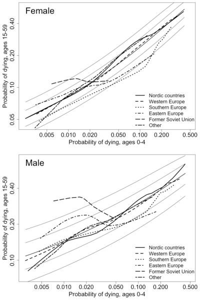
A system of model life tables defines a set of possible relationships between levels of mortality at different ages. The implied relationships for such a system can be compared to empirical reality as an elementary test of the model’s validity. In Figure 1 we compare the relationships between child and adult mortality implied by the four regional families of the Coale-Demeny system to a large body of empirical data (the dataset will be described fully later in this article). In this comparison child mortality is defined by the probability of dying between birth and age 5, or ₅q₀, and adult mortality by the (conditional) probability of dying between ages 15 and 60, or ₄₅q₁₅; in the graph both measures are displayed in a logarithmic scale.

Figure 1.

Sex-specific relationships between child and adult mortality levels (₅q₀ and ₄₅q₁₅), HMD data (n = 719) and Coale-Demeny model life tables (4 regional families)

Source: Data as summarized in Table 1a, plus Coale and Demeny (1983), UN (2000), and Buettner (2002)

Figure 1 depicts two versions of the Coale-Demeny system of model life tables. The original tables had a variable age range ending with 90, 95, or 100 and above, and an upper limit of 80 years for women’s life expectancy at birth. In preparation for the 1998 revision of official UN population estimates, this system was extended to include uniform age groups up to 100 and above, and, for females, life expectancies at birth up to 92.5 years (United Nations 2000; Buettner 2002). Such extensions were necessitated by the continuing expansion of the human life span (including projections of future trends).

For both the original and the extended versions of the Coale-Demeny model life tables, however, the relationship between child and adult mortality deviates substantially from the empirical data presented here in Figure 1, especially at lower levels of mortality (see also Coale and Guo 1989). A similar pattern is observed for the UN model life tables at relatively low levels of mortality, as documented in the supplemental report (Wilmoth et al. 2011; Figure S-5). It is worth noting that the low levels of mortality observed in recent decades were not present in the datasets used to derive the original Coale-Demeny and UN model life table systems, and thus it is not surprising that these systems (even when modified) have become increasingly inadequate as tools of mortality estimation. The bias is severe only when child mortality drops below about 50–60 per 1000. However, due to the rapid decline of mortality in less developed countries, a growing number of populations for which mortality estimates are derived using model life tables now have child mortality levels in this range. For the 2008 round of estimates from the United Nations, more than 20 countries fell into this category, including many small countries but also Indonesia, the Philippines, and Turkey.

Data from empirical life tables

For fitting the new model and testing it against alternatives, we have used life tables from several sources. Table 1 contains a summary of the four sets of life tables that were used for this study. Data from the Human Mortality Database (HMD, www.mortality.org) are described in Table 1a. This dataset contains 719 period life tables covering (mostly) five-year time intervals and represents over 72 billion person-years of exposure-to-risk, spread across parts of five continents and four centuries. All life tables in this collection were computed directly from observed deaths and population counts, without adjustment except at the oldest ages.

Table 1.

Life tables from various sources used for this analysis

a) Human Mortality Database
Country or Area	Year(s)	Number of tables	Exposure-to-risk (millions of person-years)
Australia	1921–2004	17	971
Austria	1947–2004	12	433
Belarus	1960–2007	10	459
Belgium	1841–1913, 1920–2006	33	1,200
Bulgaria	1947–2004	12	478
Canada	1921–2004	17	1,599
Chile	1992–2004	3	188
Czech Republic	1950–2006	12	567
Denmark	1835–2007	35	568
England and Wales	1841–2006	34	6,044
Estonia	1960–2007	10	68
Finland	1878–2007	27	491
France	1816–2006	39	7,909
Germany, East	1956–2006	11	841
Germany, West	1956–2006	11	3,154
Hungary	1950–2004	11	563
Iceland	1838–2007	35	22
Ireland	1950–2006	12	189
Italy	1872–2004	27	5,737
Japan	1947–2006	13	6,496
Latvia	1960–2007	10	116
Lithuania	1960–2007	10	162
Luxembourg	1960–2006	10	18
Netherlands	1850–2006	32	1,339
New Zealand	1876–2003	26	239
Norway	1846–2006	33	458
Poland	1958–2006	11	1,724
Portugal	1940–2007	14	630
Russia	1960–2006	10	6,503
Scotland	1855–2006	31	695
Slovakia	1950–2006	12	270
Slovenia	1983–2006	6	48
Spain	1908–2006	21	3,023
Sweden	1751–2007	52	1,227
Switzerland	1876–2007	27	633
Taiwan	1970–2007	8	741
Ukraine	1960–2006	10	2,288
United States	1933–2004	15	14,424
Total		719	72,517

b) WHO life table collection
Country or Area	Year(s)	Number of tables	Exposure-to-risk (millions of person-years)
Argentina	1966–1970, 1977–1979, 1982–1997	24	715
Australia	1911	1	5
Chile	1909, 1920, 1930, 1940, 1950, 1955–1982, 1984–1991	41	378
Colombia	1960, 1964	2	23
Costa Rica	1956–1983, 1985–1998	42	92
Croatia	1982–1998	17	79
Cuba	1970–1998	29	290
Czechoslovakia	1934	1	15
El Salvador	1950, 1971	2	13
Georgia	1981–1992, 1994–1996	15	77
Greece	1928, 1956–1998	44	404
Guatemala	1961, 1964	2	8
Honduras	1961, 1974	2	15
India	1971	1	1,685
Iran (Islamic Republic of)	1974	1	131
Israel	1975–1998	24	108
Matlab (Bangladesh)	1975	1	1
Mauritius	1990–1998	9	10
Mexico	1958–1959, 1969–1973, 1981–1983, 1985–1998	24	1,763
Moldova	1981–1998	18	76
Panama	1960	1	1
Peru	1970	1	40
Philippines	1964, 1970	2	141
Portugal	1920, 1930	2	13
Republic of Korea	1973	1	170
Romania	1963, 1969–1978, 1980–1998	30	660
Singapore	1955–1998	44	100
Slovenia	1982	1	2
South Africa (colored pop.)	1941, 1951, 1960	3	3
Sri Lanka	1946, 1953	2	45
Taiwan, Province of China	1920, 1930, 1936	3	29
Thailand	1970	1	112
The former Yugoslav Republic of Macedonia	1982–1997	16	32
Trinidad and Tobago	1990–1995, 1997	7	9
Tunisia	1968	1	10
United States of America	1900–1916, 1920–1932	30	2,039
Yugoslavia	1982–1997	16	166
Sub-total WHO 1802 only	--	461	9,460
Overlap with HMD	--	1,341	43,075
Total	--	1,802	52,535

c) INDEPTH life tables
Population aggregate	Year(s)	Number of tables	Exposure-to-risk (millions of person-years)
Africa, low HIV	1995–1999	8	1.7
Africa, high HIV	1995–1999	9	2.3
Bangladesh (Matlab)	1995–1999	2	0.2
Total	--	19	4.2

d) Human Life-Table Database
Country or Area	Year(s)	Number of tables	Exposure-to-risk (millions of person-years)
Austria	1865–1882,1889–1892,1899–1912,1930–1933	10	221.7
Bahrain	1998	1	0.6
Bangladesh	1974, 1976–1989,1991–1994,1996	22	2,014.2
Brazil	1998–2004	7	1,236.9
Bulgaria	1900–1905	1	23.3
China	1981	29	1,012.0
Czech Republic	1920–1933, 1935–1949	29	391.0
Egypt	1944–1946	1	54.9
Estonia	1897,1922–1923,1932–1934,1958–1959	4	8.9
Gaza Strip	1998	1	1.1
Germany	1871–1911,1924–1926,1932–1934	8	2,481.2
Germany, former Dem. Rep.	1952–1955	3	72.2
Germany, former Fed. Rep.	1949–1951	1	208.0
Greece	1926–1930,1940	2	38.4
Greenland	1971–2003	9	1.8
India	1901–1999	46	45,646.4
Iraq	1998	1	23.7
Ireland	1925–1927,1935–1937,1940–1942,1945–1947	4	35.6
Israel	1997–2005	20	55.8
Jordan	1998	1	4.6
Kuwait	1998	1	2.0
Lebanon	1998	1	3.7
Luxembourg	1901–1959	59	16.5
Malta	2001,2003–2005	4	1.6
Mexico	1980	1	69.3
Oman	1998	1	2.3
Poland	1922,1927,1948,1952–1953	4	134.1
Qatar	1998	1	0.6
Republic of Korea	1970,1978–1979,1983,1985–1987,1989,1991	8	355.8
Russia	1956–1959	4	463.1
Saudi Arabia	1998	1	19.7
Slovenia	1930–1933,1948–1954,1960–1962,1970–1972, 1980–1982	6	30.2
South Africa	1925–1927,1969–1971	3	90.7
Spain	1900	1	18.6
Sri Lanka	1963,1971,1980–1982	3	68.6
Syria	1998	1	15.7
Taiwan	1926–1930,1936–1940,1956–1958,1966–1967	4	104.8
USSR	1926,1927,1938,1939,1958,1959	3	1,047.1
United Arab Emirates	1998	1	2.9
United Kingdom, N. Ireland	1980–2003	22	38.8
United States of America	1917–1919	3	309.3
Uruguay	2005	1	3.3
Venezuela	1941–1942,1950–1951	2	18.1
West Bank	1998	1	1.6
Yemen	1998	1	17.1
Total	--	337	56,367.8

Notes:

1. Life tables by sex are counted only once. Throughout Table 1, we count a maximum of one life table per country-period.
2. If the death counts used to construct the life table come from more than one year, we count exposure-to-risk over the full period.
3. Data for New Zealand refer to the non-Maori population prior to 1950 and to the full national population after 1950.

Source: Human Mortality Database, www.mortality.org (accessed 4 February 2009)

Notes:

1. Life tables in this collection that overlap with the HMD (Table 1a) are not listed here individually.
2. The complete collection of life tables was used by Murray et al. (2003) in creating the modified logit model and life table system.

Source: Murray et al. (2003)

Source: INDEPTH network (2002)

Notes:

1. Person-year estimates are based on historical population data for each area. If the death counts used to construct the life table come from more than one year, we count exposure-to-risk over the full period.
2. For some areas, life tables represent subpopulations.
3. Life tables from the HLD that overlap with those in the HMD or the WHO collection (see Tables 1a and 1b) are not listed here.

Source: Human Life-Table Database, www.lifetable.de (accessed 20 May 2008)

HMD data have been corrected for obvious errors in published data sources: for example, an entry of ‘30,000’ that clearly should have been ‘300’ (such corrections are often confirmed by marginal totals). Errors due to misreporting of age have generally not been corrected. Only for the oldest ages (above age 95, approximately), a fitted curve following the Kannisto model (Thatcher et al. 1998) assures smoothness and, in some cases, a more plausible trajectory of old-age mortality. A convenient feature is that all HMD data are available up to an open interval of age 110 and above.

A large collection of life tables was assembled by the World Health Organization a few years ago and was subsequently used for creating a modified form of the Brass logit model of human survival (Murray et al. 2003). This data source is summarized in Table 1b. However, for both this and the following collections of life tables, we have omitted data for countries and time periods that are covered by the HMD. The non-overlapping portion of the WHO life table collection consists mostly of life tables computed directly from data on deaths and population size, which were taken (without adjustment) from the WHO mortality database (the current version of this database is available at www.who.int/healthinfo/morttables/en). Many of these life tables are for countries of Latin America and the Caribbean. A much smaller number of tables were taken from two earlier collections of life tables: those assembled by Preston and his collaborators (Preston et al. 1972), and those used for constructing the UN model life tables for less developed countries (United Nations 1982). Many of the life tables in the UN collection were derived using some form of data adjustment or modeling intended to correct known or suspected errors, or both. The mortality estimates in the Preston collection are unadjusted and may contain biases due to flawed data. All data in the WHO collection are available in standard five-year age categories, with an open interval for ages 85 and above.

In Table 1c we summarize a collection of 19 published life tables from the INDEPTH project, which has brought together data from demographic surveillance sites located in Africa and elsewhere (INDEPTH network 2002). In these surveillance areas, complete demographic data are collected for relatively small and well-defined populations. All except two of these tables refer to African sites; the other two refer to the Matlab areas (treatment and control) of Bangladesh. The INDEPTH life tables used here refer to a time period of 1995–99 (approximately) and were computed directly from observed data without adjustment.

Data from the Human Life-Table Database (HLD, www.lifetable.de) are summarized in Table 1d (after removing all overlap with the HMD and WHO collections). These life tables form a disparate collection of data from various countries and time periods. Due to the variety of data sources, the format of the data is not highly standardized. We assembled a uniform set of key mortality indicators (e₀, ₁q₀, ₅q₀, ₄₅q₁₅, and ₂₀q₆₀) for testing the new mortality model, but those are the only data from the HLD that were used for this project. Although we have not checked all sources closely, we suspect that many of these tables were constructed using some form of data adjustment or model fitting (at both younger and older ages).

Log-quadratic mortality model

Here, we consider the following model of the relationship between the death rate at age x, m_x, and the probability of dying between birth and age 5, ₅q₀, for some population at a point in time:

$$log(m_x)=a_x+b_{x}h+c_x{h}^2+v_{x}k.$$ (1)

In this model, h equals log(₅q₀) and has a quadratic relationship with the logarithm of mortality rates by age; k is real number typically in the range of (−2, 2) and depicts the magnitude and direction of deviations from a typical age pattern of mortality. In practice, the subscript x refers to the following age groups: 0, 1–4, 5–9, 10–14, …, 105–109, 110+. Values of h and k are held constant across the life span, and thus two parameters fully determine the level and shape of a predicted mortality curve (given age vectors of a_x, b_x, c_x, and v_x).

In applications of this model, the h parameter serves as the first (and primary) entry parameter for the model life table system and determines the overall level of mortality. This formulation reflects the fact that ₅q₀ is the only mortality statistic for which some empirical information is available in recent decades for almost all national populations. The second entry parameter, k, affects the shape of the age pattern of mortality and has a typical (or default) value of zero. After estimating the model (see next section), it becomes apparent that the k parameter depicts the relative excess of adult mortality (especially for ages 15–59) compared to what one might predict based on knowledge of child mortality (₅q₀) alone.

The model proposed here is similar to an earlier proposal by Wilmoth et al. (2006). The form of the new model was motivated by an empirical finding of approximate linearity in the relationship between mortality levels for various age groups, when mortality rates or probabilities of dying are expressed in a logarithmic scale. Indeed, much of the variation in the observed data can be described by the first portion of the log-quadratic model, a_x + b_xh, which depicts a linear relationship in a log-log scale. A similar log-linear relationship forms the basis of a popular method of mortality forecasting (Lee and Carter 1992). Correlation coefficients between log(_nm_x) and log(₅q₀) are reported here in Table 2. Note that these correlations are much higher at younger ages and near zero at the oldest ages.

Table 2.

Correlation coefficients, age-specific death rates vs. probability of dying under age 5 (both in logarithmic scale), Human Mortality Database life tables (n = 719)

Age group	Female	Male
0	0.983	0.984
1–4	0.969	0.963
5–9	0.944	0.935
10–14	0.944	0.940
15–19	0.936	0.900
20–24	0.939	0.768
25–29	0.949	0.829
30–34	0.958	0.871
35–39	0.961	0.883
40–44	0.962	0.874
45–49	0.947	0.845
50–54	0.942	0.814
55–59	0.930	0.774
60–64	0.942	0.775
65–69	0.928	0.772
70–74	0.912	0.798
75–79	0.873	0.779
80–84	0.812	0.747
85–89	0.713	0.658
90–94	0.565	0.473
95–99	0.378	0.363
100–104	0.155	0.218
105–109	−0.045	0.093
110+	−0.174	0.004

Note: Table shows correlations between log(_nm_x) and log(₅q₀).

Source: Data as summarized in Table 1a

Dropping the quadratic term from the model of equation (1), we obtain a log-linear variant:

$$log(m_x)=a_x+b_{x}h+v_{x}k.$$ (2)

Figure 2 shows how the log-quadratic model captures curvature in the relationship between log(_nm_x) and log(₅q₀) that is not reflected in the more parsimonious log-linear model (with k = 0 in both cases). The quadratic curves in Figure 2 tend to bend upward at younger ages (except age 0) and downward at older ages. The superior performance of the log-quadratic model compared to the log-linear variant is also reflected in measures of goodness-of-fit presented later in this article.

Figure 2.

Age-specific death rates (_nM_x) vs. child mortality (₅q₀) in a log-log scale, with predictions of log-linear and log-quadratic models for k = 0, total population (sexes combined)

Source: As for Table 3

In addition to some curvature in the expected relationship between log(_nm_x) and log(₅q₀), deviations from exact quadratic relationships tend to occur simultaneously and in a similar fashion across age groups for the same population. In the estimated model, the co-variation across age of such deviations is captured by v_xk, where the v_x vector depicts the age pattern of typical deviations in log-mortality from the expected quadratic form (i.e., for k = 0), and the value of k determines the direction and magnitude of this deviation.

Fitting the model to observed data

The log-quadratic model has been fitted separately by sex using various methods applied to a collection of 719 sex-specific life tables from the Human Mortality Database (see Table 1). All of these life tables have the same configuration of age groups (0, 1–4, 5–9, 10–14, …, 105–109, 110+), and almost all of them refer to five-year time periods.

The fitting procedure using ordinary least squares (OLS) is quite simple. It consists of fitting a series of quadratic regressions of log(_nm_x) as a function of log(₅q₀), in order to obtain the estimated coefficients, â_x, b̂_x, and ĉ_x. Each of these separate regressions results in a predicted curve describing the relationship between log(₅q₀) and log(_nm_x) for each age group, as depicted in Figure 2 for broad age groups. (Several variants of Figure 2 are shown in Figures S-6, S-7, and S-8 of the supplemental report.) In a second step, the last set of estimated coefficients, v̂_x, are obtained from the first term of a singular value decomposition, computed from the matrix of regression residuals. This term captures the common tendency toward positive co-variation (of unusually high or low mortality rates) for adjacent age groups, especially in the prime adult years.

Although somewhat more complicated than OLS, our preferred fitting procedure involves a form of weighted least squares in which we assign progressively less weight to observations with larger residual values. Compared to ordinary least squares, the difference in fitted values by our preferred method is negligible except for ages 15–59 among males and ages 15–29 among females. The estimated coefficients based on our preferred fitting method for the log-quadratic model are reported here in Table 3. Both the OLS method and our preferred fitting procedure are described fully in the Appendix. The supplemental report mentioned earlier provides the estimated coefficients for the log-linear model (Table S-1) and information about alternative fitting procedures that we considered (under “Alternative fitting methods”).

Table 3.

Coefficients for log-quadratic model, estimated using HMD life tables (n = 719)

Age	Female				Male
	ax	bx	cx	vx	ax	bx	cx	vx
0	−0.6619	0.7684	−0.0277	0.0000	−0.5101	0.8164	−0.0245	0.0000
1–4	--	--	--	--	--	--	--	--
5–9	−2.5608	1.7937	0.1082	0.2788	−3.0435	1.5270	0.0817	0.1720
10–14	−3.2435	1.6653	0.1088	0.3423	−3.9554	1.2390	0.0638	0.1683
15–19	−3.1099	1.5797	0.1147	0.4007	−3.9374	1.0425	0.0750	0.2161
20–24	−2.9789	1.5053	0.1011	0.4133	−3.4165	1.1651	0.0945	0.3022
25–29	−3.0185	1.3729	0.0815	0.3884	−3.4237	1.1444	0.0905	0.3624
30–34	−3.0201	1.2879	0.0778	0.3391	−3.4438	1.0682	0.0814	0.3848
35–39	−3.1487	1.1071	0.0637	0.2829	−3.4198	0.9620	0.0714	0.3779
40–44	−3.2690	0.9339	0.0533	0.2246	−3.3829	0.8337	0.0609	0.3530
45–49	−3.5202	0.6642	0.0289	0.1774	−3.4456	0.6039	0.0362	0.3060
50–54	−3.4076	0.5556	0.0208	0.1429	−3.4217	0.4001	0.0138	0.2564
55–59	−3.2587	0.4461	0.0101	0.1190	−3.4144	0.1760	−0.0128	0.2017
60–64	−2.8907	0.3988	0.0042	0.0807	−3.1402	0.0921	−0.0216	0.1616
65–69	−2.6608	0.2591	−0.0135	0.0571	−2.8565	0.0217	−0.0283	0.1216
70–74	−2.2949	0.1759	−0.0229	0.0295	−2.4114	0.0388	−0.0235	0.0864
75–79	−2.0414	0.0481	−0.0354	0.0114	−2.0411	0.0093	−0.0252	0.0537
80–84	−1.7308	−0.0064	−0.0347	0.0033	−1.6456	0.0085	−0.0221	0.0316
85–89	−1.4473	−0.0531	−0.0327	0.0040	−1.3203	−0.0183	−0.0219	0.0061
90–94	−1.1582	−0.0617	−0.0259	0.0000	−1.0368	−0.0314	−0.0184	0.0000
95–99	−0.8655	−0.0598	−0.0198	0.0000	−0.7310	−0.0170	−0.0133	0.0000
100–104	−0.6294	−0.0513	−0.0134	0.0000	−0.5024	−0.0081	−0.0086	0.0000
105–109	−0.4282	−0.0341	−0.0075	0.0000	−0.3275	0.0001	−0.0048	0.0000
110+	−0.2966	−0.0229	−0.0041	0.0000	−0.2212	0.0028	−0.0027	0.0000

Notes:

1. Estimated coefficients shown here were derived using the bi-weight method (see Appendix).
2. There are no estimated coefficients for ages 1–4 by design. Since ₅q₀ is an input to the model, the age group 1–4 is excluded when fitting the model. After using the model to estimate mortality for age 0, we derive the mortality level for ages 1–4 as a residual component of ₅q₀. This procedure assures that the input and output values of ₅q₀ are identical.

Source: Authors’ calculations using data as summarized in Table 1a

Choice of dataset used for fitting the model

The estimated coefficients for the log-quadratic model shown in Table 3 were derived using data drawn exclusively from the Human Mortality Database (HMD). After weighing various options, we chose to fit the model using only these data, but to test it using data from several available sources. The first choice is somewhat controversial, since the HMD dataset includes life tables for only two populations in less developed regions of the world (Taiwan and Chile), whose mortality experience is not typical of most less developed countries, and because there is only one large country (Japan) with a majority population of non-European origin. This feature of our analysis raises the question of the whether the fitted model is appropriate for use in estimating the mortality patterns of less developed countries.

To address this issue, let us begin by noting that the choice of a dataset in this context is inherently difficult and may have no perfect solution. On the one hand, it is important to derive the model using accurate information about the age pattern of mortality. On the other hand, it is also important to derive the model using data that are representative of the full range of true mortality patterns occurring throughout the world. Since the quality of available information tends to be much lower in less developed countries (in terms of the completeness and reliability of data collected through vital registration and periodic censuses), a tradeoff between the accuracy and representativeness of the data used for fitting the model is unavoidable.

The choice to fit the new model using only the HMD dataset was made for several reasons. Three of these reasons are related to certain desirable properties of the HMD dataset itself. First, the dataset is well documented, which helps to assure that the empirical basis of the model will be, if not fully transparent, at least readily accessible. Second, to minimize transcription errors, HMD life tables are derived using data obtained directly from national statistical offices or their regular publications, and data preparation includes procedures designed to detect gross errors and other anomalies. Third, age-specific mortality rates are computed directly from official data, without major adjustment or use of fitted models except for the oldest ages. One consequence of this approach is that countries and time periods included in the HMD have in principle been filtered according to the quality of the available statistical information. By these criteria alone, however, the additional life tables considered here (see Tables 1b, 1c, and 1d) would be less desirable than the HMD data but not necessarily without value.

As a practical matter, the differing age formats of the various life tables presented a minor or a serious obstacle, depending on the case. In order to combine the various life table collections to enable a joint analysis, a common age format was needed. However, to avoid sacrificing the age detail available in the HMD, it was necessary to extend the age groupings of other tables so that they, too, would end with an age category of 110+. For the HLD tables, the variety of age formats that are present in the data would have necessitated a considerable effort in order to create tables with uniform age categories, and thus they were not considered as inputs for estimating the model. By contrast, the life tables of the WHO and INDEPTH collections have uniform age groupings up to age 85, and we were able to extend the age range to 110+ by fitting the Kannisto model of old-age mortality to the available data and then extrapolating the fitted curve to higher ages. (The Kannisto model implies that death rates at older ages follow a simple logistic curve with an upper asymptote of one.) The extended life tables were combined with the HMD data to produce alternative fittings of the log-quadratic model. The alternative estimates differ little from our preferred estimates except at the oldest ages, where data from the WHO and INDEPTH tables were derived by extrapolating mortality rates from younger age groups. (See Figure S-1 of the supplemental report.)

For these reasons we decided to estimate the new model using a more restricted dataset, but to test the resulting model life table system using data from a wide variety of populations. We must bear in mind that any failed test may indicate problems with the data or with the model.

Mortality estimation using the fitted model

As an estimation tool, the log-quadratic model can be used to derive a full life table given either one or two pieces of information. In the first case, one assumes that the only reliable data that are available refer to child mortality, expressed in the form of ₅q_0. Lacking independent information about adult mortality, the simplest approach is to assume that k = 0. In the two-parameter case, one assumes that information is also available about adult mortality. For this discussion we focus on ₄₅q₁₅, though another summary measure of adult mortality could be used (e.g., ₃₅q₁₅). Thus, for a given set of age-specific coefficients and a known value of ₅q₀, we choose a value of k in order to reproduce the observed value of ₄₅q₁₅ exactly. Calculation of k in this situation is fairly simple but requires an iterative procedure. Note that we fitted the model to the HMD dataset using the usual least squares criterion of the singular value decomposition; therefore, the fit is not optimized for ₄₅q₁₅ in particular. However, in using the model for the indirect estimation of mortality, we propose that k should be chosen to match an estimate of ₄₅q₁₅, if available.

Using h = log(₅q₀) and k derived in this manner, the model can be used to estimate age-specific mortality rates across the life span by application of the following formula:

$${\widehat{m}}_x=e^{{\widehat{a}}_x+{\widehat{b}}_{x}h+{\widehat{c}}_x{h}^2+{\widehat{v}}_{x}k}.$$ (3)

These rates can then be transformed into a life table, from which it is easy to derive all of the usual summary measures of mortality, including life expectancy at birth. The errors of estimation that result directly from this procedure (i.e., assuming the input values are correct) will be discussed in a later section of this article.

Age patterns of mortality implied by the model

Model age patterns of mortality are illustrated in Figure 3, which shows the effect of changes in h and k on the shape of the mortality curve as a function of age for the log-quadratic model. The first parameter, h = log(₅q₀), controls the overall level of mortality. Movements up or down in level are accompanied by progressive changes in the tilt and shape of the curve. The second parameter, k, alters the shape of the mortality curve (for a given value of ₅q₀), especially for young and middle adult ages (roughly, from the teens to the 60s). When k is greater than zero, adult mortality is relatively high given the associated value of ₅q₀, and vice versa.

Figure 3.

Typical age patterns of mortality implied by the log-quadratic model for selected combinations of the canonical input parameters (₅q₀ and k)

Source: As for Table 3

The model can be specified using various combinations of one or two pieces of information, from which we derive associated values of h and k by some computational procedure. We have written a computer program to permit calculation of the full model using various combinations of the following six inputs: ₁q₀, ₅q₀, k, ₄₅q₁₅, ₃₅q₁₅, and e₀. Any two of these quantities are sufficient to specify the model except the pairing of ₁q₀ and ₅q₀, which provides no direct information about adult mortality, or of ₄₅q₁₅ and ₃₅q₁₅, which contains no direct information about child mortality. The program (written in R) is freely available, along with pertinent data and examples, at www.mortality.org/LogQuad or [journal URL].

Figure 4 illustrates three of these possible pairings, for females on the left and males on the right. Similar graphs with all possible permutations of ₅q₀, k, ₄₅q₁₅, and e₀ are provided in the supplemental report (see Figures S-2 and S-3). In each case, these graphs show changes in the age pattern of mortality as we hold one of the two quantities constant while varying the other one. For this figure only, the age patterns have been smoothed by fitting spline functions to the predicted values of death rates in 5-year age intervals; the smoothing helps to clarify the underlying shape.

Figure 4.

Sex-specific age patterns of mortality implied by 3 selected pairs of input parameters: top panels are based on ₅q₀ and k, middle panels on k and e₀, bottom panels on e₀ and ₅q₀

Source: As for Table 3

Note: For the pair of input variables in each panel, one value is fixed and the other is variable.

This exercise demonstrates that the model is capable of reproducing a wide variety of mortality curves, but also that these curves have entirely plausible shapes so long as k stays roughly within a range of (−4, 4). In particular, the following three features of these curves are consistent with a large body of cross-cultural and historical evidence:

1. A minimum occurs regularly around ages 10–11;

2. Above age 30 each curve is fairly straight (in a log scale) but with a slight S-shape;

3. Holding k constant (see middle row panels), the “accident hump” at young adult ages is more prominent at lower levels of mortality and for men. For women, it is possible to observe a gradual transition from a “maternal mortality hump” (roughly, ages 15–45) at the highest levels of mortality, to an attenuated male-type accident hump (roughly, ages 15–25) at lower levels.

For larger values of k (beyond +/−4, approximately), the mortality curves tend to become distorted (see supplemental report, Figure S-4). For k around +/−4, these distortion are fairly minor: they yield curves that appear somewhat unusual but with little noticeable effect on calculated values of major summary indicators (such as life expectancy at birth). For more extreme values of k (say, +/−8), the curves become more severely distorted. For example, with very large negative values, the accident hump tends to disappear, and the minimum value can move to much higher ages (around age 30). Because historical values of k lie in a fairly narrow range, this parameter can serve as an important plausibility check by helping to identify unlikely combinations ₅q₀ of and ₄₅q_15.

Relationship of the model to historical evidence

Figure 5 illustrates the relationship between the two entry parameters of the log-quadratic model, ₅q₀ and k, and the level of adult mortality as measured by ₄₅q₁₅. Five curves trace the predicted relationship between ₅q₀ and ₄₅q₁₅ corresponding to k equal to −2, −1, 0, 1, or 2. These curves overlie a scatter plot of observed values of ₅q₀ and ₄₅q₁₅ from the HMD dataset that was used for estimating the model.

Figure 5.

Adult mortality (₄₅q₁₅) vs. child mortality (₅q₀), by sex, HMD data (n = 719) and log-quadratic model for 5 selected values of k

Source: As for Table 3

With an appropriate choice of k, the model is capable of reproducing any combination of ₅q₀ and ₄₅q_15. Likewise, any combination of ₅q₀ and ₄₅q₁₅ implies a unique value of k. It is notable in this regard that the values of k implied by this diverse dataset (see Table 1) lie within a fairly narrow range, only rarely departing from the interval of −2 to +2. However, there are three important exceptions.

First, in the left-hand portion of each graph, there is a cluster of points lying above the curve representing k = 2. These points correspond to certain countries of the former Soviet Union and Eastern Europe, which have experienced unusually high adult mortality in recent decades, especially among men, in the wake of massive social and political changes.

Second, a sole data point lies well above the same curve on the right-hand side of the graph for men only. This point corresponds to Finland during 1940–44 and reflects excess mortality among young men fighting in wars against the Soviet Union. In the main dataset used here for estimating the model, the Finnish case of 1940–44 is the only example of a mortality pattern for males that is substantially affected by war mortality. It was left in the dataset in order to emphasize this important point: for other countries with substantial war losses during the period covered by the dataset, the series that we have used here reflect exclusively or primarily the mortality experience of the civilian population in times of war. In such situations the age pattern of mortality for the total population of males is clearly atypical and requires a special treatment.

Third, on the right-hand side of the graph there are a few points lying below the curve representing k = −2, especially for women. The data points in this area of the graph (both slightly above and below k = −2) correspond to countries of Southern Europe during the 1950s and early 1960s (Portugal and Bulgaria are the most extreme cases), and reflect a situation of unusually low adult mortality relative to child mortality (or, put differently, unusually high child mortality relative to adult mortality). As illustrated in Figure 1, the South family of the Coale-Demeny model life table system depicted accurately the mortality experience of this region during those earlier decades; but afterward, it has deviated from the historical record as mortality fell to lower levels in these countries.

Figure 6 shows results very similar to those in Figure 5 but broken down by smaller age groups. Several variants of Figure 5 and 6 are available in the supplemental report (Figures S-9, S-10, and S-11). These graphs demonstrate that the relative impact of the k parameter on predicted levels of mortality differs for the various age groups and by sex. For both men and women, this parameter helps to distinguish between high or low levels of adult mortality (relative to child levels) throughout the age range from 15 to 59. However, in the age group of 60–79, the importance of the k parameter remains for men but diminishes substantially for women. For women at ages 60–79 and for both sexes at ages 80–99, the variability in the data vastly exceeds the variability implied by choices of k within a plausible range.

Figure 6.

Age-specific death rates (_nM_x) vs. child mortality (₅q₀) for 6 age groups, HMD data (n = 719) and log-quadratic model (for 5 values of k)

Source: As for Table 3

These results reflect the fact that the strong positive co-variation in levels of adult mortality relative to child mortality is limited to a particular age range. The variability in relative levels of mortality at older ages is not highly correlated with the variability observed at younger adult ages and is thus random variation from the perspective of this two-dimensional model. Moreover, the age range where the k parameter has a substantial impact on mortality estimates is somewhat narrower for women than for men. In times of social and political instability, when adults of both sexes are exposed to elevated risks of dying, this excess vulnerability tends to affect men both more intensely and over a broader age range compared to women.

Accuracy of estimation

We have evaluated the performance of the log-quadratic model along two dimensions. First, we compared the performance of the new model to that of methods used currently by international agencies and national statistical offices for creating official mortality estimates. Second, we compared the performance of the log-quadratic model when applied to populations included in the dataset used for deriving the model versus populations that were not part of this dataset.

Model performance was assessed in comparison to three existing methods: Coale-Demeny model life tables, UN model life tables for less developed countries, and the modified logit model. We used four datasets to make these comparisons: the HMD dataset, the INDEPTH life tables for 1995–99, and both the WHO and HLD collections (after excluding life tables that overlap with the HMD).

In order to focus attention on the models themselves (apart from the datasets used for estimating the models), we have re-estimated the modified logit model using the same HMD dataset used for fitting the log-quadratic model (see supplemental report, “Fitting algorithm for modified logit model” and Table S-2). Thus, when assessing the performance of the modified logit model, we made separate tests using the re-estimated model and the original version proposed by Murray et al. (2003).

To compare the performance of the log-linear, log-quadratic, and modified logit models, we have assessed the accuracy of life table estimates derived using ₅q₀ alone, or using ₅q₀ and ₄₅q₁₅ together as input parameters. For tests requiring ₅q₀ alone as an input, we have also included comparisons with the Coale-Demeny West and the UN General model life tables. When only information on ₅q₀ is available, estimates of l₆₀ that serve as inputs to the modified logit model were derived using a side model that depicts the empirical relationship between l₅ and l₆₀, following a method used by the WHO in applications of the model (additional details are available in the supplemental report).

Comparisons of the log-quadratic model with the Coale-Demeny and UN model life tables are somewhat more complicated, since the latter have discrete regional families rather than a continuous second parameter. Therefore, to more fully compare these model life table systems to a system based on the log-quadratic model, we have created five “families” of the latter model corresponding to specific values of the k parameter (for k = 2, −1, 0, 1, and 2). Given ₅q₀ alone, we derived a complete set of age-specific death rates and an associated life table for each region or family of the various model systems. Then, within each model system we chose the “best” region or family as the one that produced the closest match to the observed ₄₅q₁₅. For the Coale-Demeny model life tables, this procedure often results in substantial underestimates of ₄₅q₁₅, especially for low values of ₅q₀ (see Figure 1).

When child mortality is at least moderately low, e₀ is less affected by child mortality and is more sensitive to variations in adult mortality. Therefore, we have also examined estimation accuracy following the reverse of the procedure described above. That is, for each family or region, we chose the level based on ₄₅q₁₅ and derived a complete life table. Then, within each model system, we chose the best region or family based on the closeness of observed and predicted values of ₅q_0.

We have assessed the accuracy of an estimation procedure by computing the root-mean-squared-error (RMSE) for four key mortality indicators: e₀, ₁q₀, ₄₅q₁₅, and ₂₀q₆₀. The results of all tests using the HMD dataset are given in Table 4. The log-quadratic model and the re-estimated modified logit model perform quite similarly in these tests, and both models produce more accurate estimates of e₀, ₄₅q₁₅, and ₂₀q₆₀ than those derived using the Coale-Demeny West or UN General model life tables. Not surprisingly, the log-quadratic model performs better than the log-linear model, and the re-estimated modified logit model has an advantage over the original version in this set of tests.

Table 4.

Root-mean-squared-errors (RMSEs) for e₀, ₁q₀, ₄₅ q₁₅, and ₂₀q₆₀ by sex, various model life table methods, Human Mortality Database life tables (n = 719)

	Female				Male
	e0	1q0	45q15	20q60	e0	1q0	45q15	20q60
Given 5q0 only:
Log-linear (bi-weight)	1.64	0.011	0.032	0.046	2.62	0.012	0.064	0.057
Log-linear (OLS)	1.67	0.010	0.033	0.047	2.60	0.011	0.062	0.057
Log-quadratic (bi-weight)	1.62	0.010	0.032	0.045	2.55	0.011	0.062	0.056
Log-quadratic (OLS)	1.62	0.010	0.032	0.045	2.52	0.011	0.060	0.056
Modified logit (re-est.)	1.66	0.010	0.032	0.048	2.47	0.011	0.060	0.052
Modified logit (orig.)	1.85	0.015	0.034	0.051	2.56	0.019	0.067	0.053
Coale-Demeny West Model	2.73	0.010	0.042	0.062	4.09	0.011	0.086	0.088
UN General Model	4.50	0.011	0.070	0.110	5.67	0.010	0.104	0.139
Given 5q0 and 45q15:
Log-linear (bi-weight)	0.83	0.011	0	0.047	0.69	0.012	0	0.045
Log-linear (OLS)	0.78	0.010	0	0.046	0.62	0.011	0	0.045
Log-quadratic (bi-weight)	0.70	0.010	0	0.042	0.59	0.011	0	0.041
Log-quadratic (OLS)	0.70	0.010	0	0.042	0.57	0.011	0	0.041
Modified logit (re-est.)	0.69	0.010	0	0.042	0.61	0.011	0	0.043
Modified logit (orig.)	0.88	0.014	0	0.045	0.99	0.020	0	0.044
Best family given 5q0:
Log-quadratic (5 families)	0.94	0.010	0.013	0.042	1.18	0.011	0.027	0.044
Coale-Demeny (4 families)	2.45	0.010	0.026	0.061	3.90	0.014	0.077	0.084
UN tables (5 families)	3.26	0.013	0.030	0.084	3.48	0.011	0.066	0.080
C-D or UN (9 families)	2.41	0.011	0.023	0.062	3.39	0.013	0.064	0.077
Best family given 45q15:
Log-quadratic (5 families)	0.99	0.013	0	0.041	1.61	0.017	0	0.042
Coale-Demeny (4 families)	1.44	0.014	0	0.052	3.12	0.032	0	0.051
UN tables (5 families)	1.37	0.016	0	0.047	1.92	0.018	0	0.062
C-D or UN (9 families)	1.37	0.013	0	0.053	1.79	0.019	0	0.062

Notes:

1. For these comparisons, the log-quadratic model was estimated using either ordinary least squares (OLS) or weighted least squares using a bi-square weight function of residuals: the bi-weight method. See Appendix for more explanation.
2. Estimation errors for the log-quadratic model in the two sets of “best family” comparisons were derived using the model as estimated by the bi-weight method.

Source: As for Table 3

Table 4 also illustrates that the five families of the log-quadratic model (based on five values of k) produce much better estimates of e₀ and ₂₀q₆₀ than do the regional variants of the Coale-Demeny or UN model life tables, or a combination of the two, whether ₅q₀ or ₄₅q₁₅ is used as the primary input parameter (in the procedures described above). For the Coale-Demeny and UN model life tables, using ₄₅q₁₅ to choose the mortality level within families and then ₅q₀ to choose the best family produces more accurate estimates than the reverse procedure.

As illustrated in Table 5, the results of tests using the HLD, INDEPTH, and WHO collections of life tables are similar to those using the HMD dataset. Again, the accuracy of estimates of e₀, ₁q₀, ₄₅q₁₅, and ₂₀q₆₀ is similar when using the log-quadratic model or the modified logit model (in either its original or re-estimated form). Tests based on the WHO dataset indicate a slight advantage for the original modified logit, reflecting the fact that the model was derived using this same dataset. Similarly, performance tests using the HLD and INDEPTH datasets sometimes indicate a slight advantage for the original modified logit (see later discussion).

Table 5.

Root-mean-squared-errors (RMSEs) for e₀, ₁q₀, ₄₅ q₁₅, and ₂₀q₆₀ by sex, various model life table methods, other (non-HMD) life tables

	Female				Male
	e0	1q0	45 q 15	20q60	e0	1q0	45 q 15	20q60
WHO-1802 life tables
Given 5q0 only:
Log-quadratic	2.63	0.007	0.045	0.069	2.86	0.007	0.056	0.083
Modified logit (re-est.)	2.64	0.007	0.043	0.075	2.96	0.007	0.057	0.087
Modified logit (orig.)	2.36	0.008	0.041	0.067	2.70	0.008	0.056	0.085
Given 5q0 and 45q15:
Log-quadratic	1.13	0.007	0	0.072	1.00	0.007	0	0.066
Modified logit (re-est.)	1.06	0.007	0	0.057	0.91	0.007	0	0.059
Modified logit (orig.)	0.92	0.008	0	0.050	0.77	0.009	0	0.059
INDEPTH life tables
Given 5q0 only:
Log-quadratic	4.06	0.032	0.111	0.139	3.72	0.037	0.122	0.127
Modified logit (re-est.)	4.07	0.027	0.109	0.150	3.93	0.032	0.131	0.129
Modified logit (orig.)	3.93	0.034	0.112	0.133	4.13	0.043	0.127	0.126
Given 5q0 and 45q15:
Log-quadratic	2.70	0.032	0	0.139	2.02	0.037	0	0.132
Modified logit (re-est.)	2.24	0.028	0	0.151	1.95	0.030	0	0.139
Modified logit (orig.)	1.75	0.034	0	0.136	1.48	0.042	0	0.137
Human Life-table Database
Given 5q0 only:
Log-quadratic	2.39	0.011	0.059	0.060	2.78	0.010	0.063	0.057
Modified logit (re-est.)	2.48	0.012	0.058	0.060	2.73	0.011	0.062	0.055
Modified logit (orig.)	2.33	0.013	0.058	0.064	2.72	0.013	0.066	0.056
Given 5q0 and 45q15:
Log-quadratic	0.90	0.011	0	0.061	0.89	0.010	0	0.048
Modified logit (re-est.)	0.77	0.015	0	0.053	0.83	0.012	0	0.046
Modified logit (orig.)	0.77	0.014	0	0.057	0.91	0.014	0	0.046

Notes:

1. In this table the log-quadratic model was estimated using the bi-weight method.
2. For the modified logit model, two versions are shown here: the “original” model with coefficients as estimated by Murray et al. (2003), and a new “re-estimated” version derived from the HMD dataset used here for fitting the log-quadratic model.
3. For tests with the HLD database, certain life tables are excluded (n=43) in the results for ₂₀q₆₀ because they do not have the requisite data.

Source: Authors’ calculations using data as summarized in Tables 1b, 1c, and 1d

Estimation errors for e₀ based on the HMD dataset are plotted in Figure 7. Each panel shows error bands corresponding to one or two times the RMSE. Note that these bands are rather narrow when two data inputs are used (bottom panels): given both ₅q₀ and ₄₅q₁₅, model predictions of e₀ lie within about 1–1.5 years of the observed value. However, when ₅q₀ is the only input (top panels), the error bands are much wider especially for males: in this case, model predictions of e₀ for women fall within about +/−3 years of the actual values whereas for men the errors have a range of roughly +/−5 years.

Figure 7.

Estimation errors of log-quadratic model for life expectancy at birth by sex, with error bands of +/−1 or 2 root-mean-squared-errors (RMSEs): top panels are for 1-dimensional model (k = 0), bottom panels are for 2-dimensional model (k to match ₄₅q₁₅), HMD data (n = 719)

Source: As for Table 3

Discussion

Comparison to other models

Based on the comparisons presented in the last section, we conclude that the log-quadratic model produces more precise mortality estimates than either the Coale-Demeny or UN model life tables and that the precision of the log-quadratic model is on a par with that of the modified logit procedure. Estimation accuracy is only one criterion, however, and we contend that there are in fact several reasons for preferring the model proposed here over currently available methods as a tool of mortality estimation.

A key advantage of the log-quadratic model over the Coale-Demeny and UN models is that the new model has two continuous parameters, rather than a single continuous parameter with a limited choice of “regional” variants. In one set of tests, we have discounted this advantage by comparing the Coale-Demeny and UN model life tables to five families of the log-quadratic model based on discrete values of the k parameter (k = −2, −1, 0, 1, 2). Our tests cannot determine whether the five families of the log-quadratic model outperform these other models because we used a more comprehensive and recent collection of mortality data, or because the structure of the new model itself is superior. Unlike our comparison with the modified logit model, it was not practical to re-estimate the Coale-Demeny or UN models using the HMD dataset because of the arbitrary nature of the regional groupings. In contrast, as new data become available in the future, it will be feasible to update (or re-calibrate) the log-quadratic model. In addition to the detailed description of methods used for fitting the log-quadratic model given here in the appendix, we are making available a set of R programs that other researchers can use to re-estimate the model, if desired, using an alternative or updated set of input life tables (see www.mortality.org/LogQuad or [journal URL]).

The log-quadratic and the modified logit models perform similarly because both have very flexible functional forms, include two continuous parameters, and have been estimated using recent and comprehensive mortality data sets. In our opinion the advantage of the log-quadratic model over the modified logit model stems from its interpretability, its flexibility, and its ease of use. For example, faced with estimating a life table for a population where the only available information pertains to child mortality, the log-quadratic model can be used directly with a single input, ₅q₀, to estimate a full set of age-specific mortality rates. In contrast, for the modified logit model in the same situation, a side model must be used first to predict the relationship between l₅ and l₆₀ before the main model can be applied. Furthermore, if a reliable independent estimate of adult mortality is not available, with the log-quadratic model there is the possibility of incorporating qualitative information (perhaps from epidemiologic studies, or from data for sub-national populations) as a means of choosing a plausible non-zero value for k. Familiarity with the historical range of estimated values of k and knowledge of specific examples (see later discussion of Figures 9 and 10) can also be used to inform such a choice.

Figure 9.

Six examples of historical mortality curves from HMD data, with predictions derived using the log-quadratic model: given ₅q₀ only (solid line), or given both ₅q₀ and ₄₅q₁₅ (dashed line)

Source: As for Table 3

Figure 10.

Adult mortality (₄₅q₁₅) vs. child mortality (₅q₀), typical regional patterns plus five families of log-quadratic model (for values of k equaling −2, −1, 0, 1, and 2)

Source: As for Table 3

Note: Regional trend lines were derived by local smoothing of all data points for countries in the region using the lowess technique. The lowess bandwidth (fraction of points included in each local smoothing) varied as a function of the range of log(₅q₀) for each data series: it was set equal to 1.3 divided by this range, yielding smaller bandwidths for longer series.

Data quality issues

One potential advantage of the modified logit over the log-quadratic model is that the WHO data set used to estimate the former model contained more life tables from less developed countries. We explored an alternative means of fitting the log-quadratic model using data from both the HMD and the WHO collections of life tables. Adding the (non-overlapping) WHO life tables to the HMD dataset had almost no impact on the fitted model (see supplemental report, Figure S-1). The only noticeable difference induced by this change was that predicted values of old-age mortality (especially above age 80) moved slightly downward. This shift seems undesirable for two reasons. First, the impact of the additional life tables on the estimated model occurs mostly above age 80, yet the additional data points above age 85 are not observed values but rather the product of an extrapolative procedure. Second, the slight reduction in fitted values may reflect nothing more than common flaws affecting unadjusted mortality data at older ages, especially in countries with less reliable statistical systems.

Age misreporting is a well-known problem in mortality estimation, especially at older ages, where the resulting bias is always downward (Coale & Kisker 1990; Preston et al. 1999). Figure 8 is informative in this regard, as it shows our preferred estimates of the log-quadratic model (derived using HMD data alone) alongside mortality estimates from the WHO and INDEPTH collections for ages 15–59 and 60–79. In the younger age range, observations from the two latter datasets lie within a plausible range according to the model. At older ages, however, the WHO and INDEPTH data are shifted downward relative to the model. We believe that the first result confirms that the log-quadratic model is applicable to a wide variety of human populations. At the same time, we believe that the second result is more likely due to imperfections in mortality data at older ages than to some limitation of the new model.

Figure 8.

Adult and old-age mortality (₄₅q₁₅ and ₂₀q₆₀) vs. child mortality (₅q₀) for various less developed country populations, compared to predictions of the log-quadratic model

Source: Data as summarized in Tables 1b and 1c

Note: For data in all three groups, large symbols refer to ₄₅q₁₅ and small symbols to ₂₀q₆₀.

Performance of the model in exceptional circumstances

Figure 9 presents six historical examples for the purpose of demonstrating the capabilities of the log-quadratic model as well as its limitations. These examples are not typical of the vast majority of historical observations; rather, each is exceptional in one manner or another. Thus, this illustration is intended to explore the limits of the model as a means of depicting historically well-documented age patterns of mortality. Each graph in Figure 9 shows observed data in comparison to estimates derived from the log-quadratic model. Two sets of estimates were obtained by inserting observed values of either ₅q₀ alone, or ₅q₀ and ₄₅q₁₅ together, as inputs to the model. The implied values of k are reported in the graph for each set of estimates (in the one-parameter case, k = 0 by definition), along with associated values of e₀.

The top row of Figure 9 compares the age pattern of mortality for two groups of men in England and Wales during 1940–44. On the left, the total population (including active military personnel) has an age pattern that is severely distorted compared to typical mortality curves. In this case the new model is clearly incapable of mimicking the underlying pattern even with two input parameters. On the right, however, the civilian population (excluding the military population) has a more typical age profile, with only minor distortions in the observed data for men in their 20s and a value of k in the two-parameter case that remains close to zero.

Although the model may do poorly in representing the age pattern of war mortality, the other four examples in Figure 9 depict relatively extreme cases where the model performs reasonably well when both inputs are supplied correctly. The graphs in the middle row document the excess adult mortality due to the Spanish flu (for women in Denmark) and to the Spanish civil war (for men in Spain). The graphs in the bottom row illustrate extreme cases of relatively low or high adult mortality in peacetime (for, respectively, Portuguese women in the 1960s and Russian men in recent years). In these four cases, the two-parameter version of the log-quadratic model provides an imperfect, yet for most purposes adequate, depiction of the age pattern of mortality. By contrast, the one-parameter version of the model yields rather large errors both in the shape of the age pattern and in the resulting value of life expectancy at birth.

It is uncertain whether the model proposed here could provide an adequate depiction of mortality in populations heavily affected by the AIDS epidemic. If not, the model life table system proposed here could be used (like earlier systems) as a means of estimating mortality from causes other than AIDS, with estimates of AIDS mortality coming from a simulation model (as done currently for global mortality estimates from the United Nations and others). This issue requires further investigation but is beyond the scope of this article.

Broader historical insights from the model

In addition to showing much promise as an estimation tool, the model proposed here can help to sharpen our understanding of the history of mortality change. Figure 10 illustrates the average trajectory of ₅q₀ versus ₄₅q₁₅ for various regions.

As illustrated in Figure 10, the average mortality trajectories for many regions have followed a fairly regular path over time, in the sense that child and adult mortality did not deviate much from the typical relationship, which is approximately linear in a log-log scale. This group includes the Nordic countries, Western Europe, and all HMD populations from outside Europe (Chile, Taiwan, Japan, New Zealand, Australia, Canada, USA). A more detailed illustration of these trends, available in the supplemental report (Figure S-12), indicates that the approximate linear relationship is also observed for individual countries within these regions. However, patterns by country pertain only to the period covered by the HMD dataset, which is quite short in some cases (the shortest series, for Chile, begins in the early 1990s).

Figure 10 also highlights the more unusual historical trajectories of Southern and Eastern Europe, and for countries of the former Soviet Union. Southern Europe had a somewhat peculiar pattern in the 1950s and 1960s, especially among women. These countries showed a pronounced “South” pattern, as defined by Coale and Demeny (relatively low adult mortality). Historically, the trend for Eastern Europe was similar to that of Southern Europe, but more recently the pattern resembles that of the countries of the former Soviet Union, though not as dramatic. In the former Soviet areas (especially Russia), the levels of adult mortality observed for both men and women in recent periods far exceed those that are expected based on child mortality alone.

Further potential improvements

It is clear that the log-quadratic model does not fit all known age patterns of human mortality. It may be possible to improve its precision by adding third-order adjustments (i.e., highly tailored v_x profiles for special cases, such as war or epidemics). However, such developments are beyond the scope of this paper. As illustrated here, the log-quadratic model provides useful first- or second- order approximations in a wide variety of situations.

Conclusion

Using life tables from the Human Mortality Database, we have developed a new system of model life tables as a means of improving the quality and transparency of mortality estimates. This system, based on a flexible two-dimensional model, can be used to estimate full life tables given information either on child mortality only, or child and adult mortality. The new method performs better or at least as well as all existing procedures. In addition, the proposed model is better suited to the practical needs of mortality estimation, since both input parameters are continuous yet the second one is optional; and since model parameters are closely related to measures of child and adult mortality, the link between data and estimates is more transparent.

We believe that the model proposed here could serve as the basis for a new and better system of mortality estimation for populations with incomplete data. To achieve this goal, additional work will be needed to adapt the model for use in populations heavily affected by war or certain forms of epidemic disease (e.g., AIDS). For a full evaluation of the uncertainty of mortality estimates, the uncertainty created by the model itself (as illustrated here in Figure 7) should be supplemented by information about the uncertainty of model inputs, in particular of ₅q₀.

Appendix

In order to describe the procedure used for estimating the log-quadratic model, it is useful to write the model as follows:

$$log(m_{xi})=a_x+b_x{h}_i+c_x{h}_i^2+v_x{k}_i+{\epsilon }_{xi}$$ (A.1)

where i is an index for a population or an individual life table; in general i = 1, …, n, and here n = 719 (see Table 1). Thus, a_x, b_x, c_x, and v_x are age-specific parameters that are fixed across populations. Only the values of h_i and k_i vary across time and space, and in all cases $h_i=log\left({{}_{5}q}_0^i\right)$. Given h_i and k_i, the model predicts the value of the log death rate with an error of ε_xi. Fitting the model to some collection of historical data will result in age-specific parameter estimates, â_x, b̂_x, ĉ_x, and v̂_x.

We have estimated this model using a variety of techniques, which are described fully in the supplemental report. Here, we document only two methods. The first one, ordinary least squares, is the simplest and serves as a useful starting point. Our preferred method however, consists of weighted least squares using the bi-square function, as suggested by Tukey as a way of minimizing or eliminating the influence of extreme observations (Andrews et al., 1972). We refer here to the preferred procedure as the bi-weight method. As noted in the main text, differences in the fitted models resulting from these two procedures are rather small in magnitude and are concentrated in the young-to-middle adult ages (roughly, ages 15–29 for women and ages 15–59 for men).

Both methods of estimating the model involve a two-step procedure. The two methods differ only on the first step, in which the quadratic portion of the model is fitted separately to each age group. For example, when fitting the quadratic portion of the log-quadratic model by the method of ordinary least squares, we obtain estimates of a_x, b_x and c_x by minimizing the following sum of squared residuals:

$$\sum _i{\left(log(m_{xi})-a_x-b_x·h_i-c_x·h_i^2\right)}^2,$$ (A.2)

When fitting this portion of the model by the bi-weight method, estimates are obtained by minimizing a weighted sum of squared residuals,

$$\sum _i{w}_{xi}{\left(log(m_{xi})-a_x-b_x·h_i-c_x·h_i^2\right)}^2,$$ (A.3)

where the weights, W_xi, are a function of the residuals of the fitted model:

$$r_{xi}=log(m_{xi})-{\widehat{a}}_x-{\widehat{b}}_x·h_i-{\widehat{c}}_x·h_i^2.$$ (A.4)

Since the weights are a function of the residuals, an iterative procedure is required (convergence is rapid in our experience, usually involving no more than 25 iterations).

The bi-square weight function is defined as follows:

$$w_{xi}=\{\begin{array}{cc}{(1-u_{xi}^2)}^2& \text{if}\mid u_{xi}\mid <1\\ 0& \text{if}\mid u_{xi}\mid \ge 1\end{array}$$ (A.5)

where $u_{xi}=\frac{r_{xi}}{{cS}_x}$, r_xi is the residual for a particular observation, S_x is the median absolute value of the residuals for that particular age group, and c is a tuning constant. For this application, we have used c = 6 for all age groups because that choice results in a weight of zero for relatively extreme examples in the HMD dataset (for example, adult mortality rates for Russian males in recent years and Portuguese females during the 1950s/1960s receive zero weight when estimating the model by this procedure with c = 6).

For both methods, the second step involves estimating the v_xk_i term by computing a singular-value decomposition (SVD) of the resulting residual matrix:

$$\text{SVD}\left[r_{xi}\right]={\mathbf{PDQ}}^{\mathbf{T}}=d_1{\mathbf{p}}_{\mathbf{1}}{\mathbf{q}}_{\mathbf{1}}^{\mathbf{T}}+\dots$$ (A.6)

where P = [p₁, p₂, …] and Q = [q₁, q₂, …] are matrices of left- and right-singular vectors, respectively, and D is a diagonal matrix with the singular values, d₁, d₂, …, along the diagonal. Only the first term of the SVD, $d_1{\mathbf{p}}_{\mathbf{1}}{\mathbf{q}}_{\mathbf{1}}^{\mathbf{T}}$, is used for obtaining parameter estimates. Specifically, the typical age pattern of deviations from an exact log-quadratic model is depicted by the first left-singular vector; thus, the values of v̂_x are set equal to the elements of p₁. After fitting the model by these procedures, estimated values of v̂_x were set to zero for certain age groups (0, 1–4, and above 90) and in a few cases at older ages where they were slightly negative (see Table 3).

For the populations used as inputs for fitting the model (i.e., the 719 life tables of the HMD collection), the optimal value of k_i by a least-squares criterion is obtained by multiplying d₁ by the appropriate element of the first right-singular vector, q₁. However, as a practical tool for estimating the full age pattern of mortality in situations with more limited data, we propose choosing the k parameter to match ₄₅q₁₅ exactly, if that quantity is known; otherwise, we propose setting k = 0 or else making an arbitrary choice based on expert knowledge of the health and circumstances of the population.

Fitting the model using the bi-weight method rather than ordinary least squares tends to pull the k = 0 curve toward the center of the main cloud of historical data points, either by down-weighting or by completely ignoring extreme observations. By varying the value of c, we have tuned the procedure so that weights in the age range of 15–59 taper off to zero at a k value of around ±2. This choice is arbitrary but seems sensible based on the historical record.

Differences in results produced by the two estimation procedures can be summarized as follows:

• Except for very old ages (where random fluctuations play an important role), differences in predicted mortality levels are negligible except for ages 15–29 among both men and women, and ages 30–59 for men only.

• For these relatively broad age categories, differences in estimated mortality rates for a given value of k attain a maximum of 9–11 per cent over the typical range of ₅q₀; however, for some 5-year age groups among males aged 25–44, such differences reach 14–16 per cent.

• For a given value of k, differences in predicted levels of life expectancy at birth are less than 0.1 years for women but as high as 0.6 years for men.

In our opinion the model predictions resulting from the bi-weight estimation procedure are preferable. It is clear that some extreme observations (in particular, the recent experience of some Eastern European and former Soviet countries) are pulling the OLS curves upward, especially for certain adult age groups. Thus, OLS predictions of some mortality levels for the default case (when k = 0) appear to be slightly overestimated.

By some measures the bi-weight method yields a less optimal fit. As shown in Table 4 of the main text, root-mean-squared-errors are sometimes slightly greater for the bi-weight method compared to the OLS procedure. However, these differences in overall goodness-of-fit are slight and seem acceptable as a means of reducing an apparent bias in certain age groups, owing to the sensitivity of the OLS procedure to extreme historical examples. In our judgment, these extreme examples should enter into a calculation of the overall uncertainty of estimation, but they should not be allowed an undue influence on the determination of a “best” estimate.

References

- Andrews DF, Hampel FR, Tukey JW, Bickel PJ, Huber PJ, Rogers WH. Robust Estimation of Location: Survey and Advances. Princeton, NJ: Princeton University Press; 1972. [Google Scholar]
- Buettner T. Approaches and experiences in projecting mortality patterns for the oldest-old. North American Acturial Journal. 2002;6(3):14–29. [Google Scholar]
- Coale AJ, Demeny P. Regional Model Life Tables and Stable Populations. 1. New York: Academic Press; 1966. 1983, 2nd ed. [Google Scholar]
- Coale AJ, Guo G. Revised regional model life tables at very low levels of mortality. Population Index. 1989;55(4):613–43. [PubMed] [Google Scholar]
- Coale AJ, Kisker EE. Defects in data on old-age mortality in the United States: New procedures for calculating mortality schedules and life tables at the highest ages. Asian and Pacific Population Forum. 1990;4(1):1–31. [Google Scholar]
- Human Life-Table Database (HLD) [accessed 20 May 2008];Max Planck Institute for Demographic Research (Germany), University of California, Berkeley (USA), and the Institut National D’Etudes Démographiques (France) 2009 Available at www.lifetable.de.
- Human Mortality Database (HMD) [accessed 4 February 2009];University of California, Berkeley (USA), and Max Planck Institute for Demographic Research (Germany) 2009 Available at www.mortality.org or www.humanmortality.de.
- INDEPTH network. Population and Health in Developing Countries. Volume 1. Population, Health, and Survival at INDEPTH Sites. Ottawa, Canada: International Development Research Centre; 2002. [Google Scholar]
- Lee RD, Carter L. Modeling and forecasting U.S. mortality. Journal of the American Statistical Association. 1992;87(419):659–671. [Google Scholar]
- Murray CJL, Ferguson BD, Lopez AD, Guillot M, Salomon JA, Ahmad O. Modified logit life table system: Principles, empirical validation, and application. Population Studies. 2003;57(2):165–182. [Google Scholar]
- Preston SH, Keyfitz N, Schoen R. Causes of Death: Life Tables for National Populations. New York: Seminar Press; 1972. [Google Scholar]
- Preston SH, Elo I, Stewart Q. Effects of age misreporting on mortality estimates at older ages. Population Studies. 1999;53(2):165–177. [Google Scholar]
- R Development Core Team. R: A Language and Environment for Statistical Computing. Vienna, Austria: R Foundation for Statistical Computing; 2009. [Google Scholar]
- StataCorp. Stata Statistical Software: Release 9. College Station, TX: StataCorp LP; 2005. [Google Scholar]
- Thatcher AR, Kannisto V, Vaupel JW. The Force of Mortality at Ages 80 to 120. Odense, Denmark: Odense University Press; 1998. [Google Scholar]
- United Nations. Model Life Tables for Developing Countries. New York: United Nations; 1982. (Sales No. E.81.XIII.7) [Google Scholar]
- United Nations. World Population Prospects: The 1998 Revision, vol. III, Analytical Report. New York: United Nations; 2000. (Sales No. E.99.XIII.10) [Google Scholar]
- Wilmoth J, Andreev K, Sawyer C. A strategy of mortality estimation for national populations. Presented at the United Nations Expert Group Meeting on Current Issues in the Estimation of Adult Mortality; 26–27 October.New York: UN Population Division/DESA; 2006. [Google Scholar]
- Wilmoth J, Zureick S, Canudas-Romo V, Inoue M, Sawyer C. A flexible two-dimensional mortality model for use in indirect estimation: Supplemental materials 2011 [Google Scholar]
Associated Data
This section collects any data citations, data availability statements, or supplementary materials included in this article.