Multi-modal Registration for Correlative Microscopy using Image Analogies

Abstract

Correlative microscopy is a methodology combining the functionality of light microscopy with the high resolution of electron microscopy and other microscopy technologies for the same biological specimen. In this paper, we propose an image registration method for correlative microscopy, which is challenging due to the distinct appearance of biological structures when imaged with different modalities. Our method is based on image analogies and allows to transform images of a given modality into the appearance-space of another modality. Hence, the registration between two different types of microscopy images can be transformed to a mono-modality image registration. We use a sparse representation model to obtain image analogies. The method makes use of corresponding image training patches of two different imaging modalities to learn a dictionary capturing appearance relations. We test our approach on backscattered electron (BSE) scanning electron microscopy (SEM)/confocal and transmission electron microscopy (TEM)/confocal images. We perform rigid, affine, and deformable registration via B-splines and show improvements over direct registration using both mutual information and sum of squared differences similarity measures to account for differences in image appearance.

1. Introduction

Correlative microscopy integrates different microscopy technologies including conventional light-, confocal- and electron transmission microscopy (Caplan et al., 2011) for the improved examination of biological specimens. E.g., fluorescent markers can be used to highlight regions of interest combined with an electron-microscopy image to provide high-resolution structural information of the regions. To allow such joint analysis requires the registration of multi-modal microscopy images. This is a challenging problem due to (large) appearance differences between the image modalities. Fig. 1 shows an example of correlative microscopy for a confocal/TEM image pair.

Figure 1.

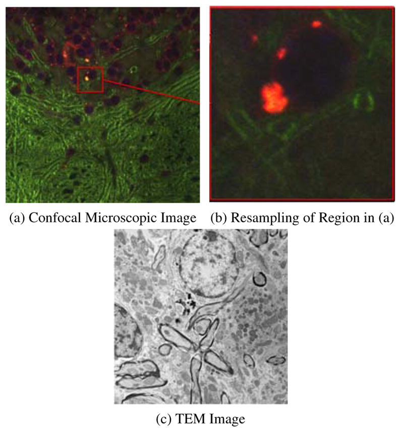
Example of Correlative Microscopy. (a) is a stained confocal brain slice, where the red box shows an example of a neuron cell and (b) is a resampled image of the boxed region in (a). The goal is to align (b) to (c).

Image registration estimates spatial transformations between images (to align them) and is an essential part of many image analysis approaches. The registration of correlative microscopic images is very challenging: images should carry distinct information to combine, for example, knowledge about protein locations (using fluorescence microscopy) and high-resolution structural data (using electron microscopy). However, this precludes the use of simple alignment measures such as the sum of squared intensity differences because intensity patterns do not correspond well or a multi-channel image has to be registered to a gray-valued image.

A solution for registration for correlative microscopy is to perform landmark-based alignment, which can be greatly simplified by adding fiducial markers (Fronczek et al., 2011). Fiducial markers cannot easily be added to some specimen, hence an alternative image-based method is needed. This can be accomplished in some cases by appropriate image filtering. This filtering is designed to only preserve information which is indicative of the desired transformation, to suppress spurious image information, or to use knowledge about the image formation process to convert an image from one modality to another. E.g., multichannel microscopy images of cells can be registered by registering their cell segmentations (Yang et al., 2008). However, such image-based approaches are highly application-specific and difficult to devise for the non-expert.

In this paper we therefore propose a method inspired by early work on texture synthesis in computer graphics using image analogies (Hertzmann et al., 2001). Here, the objective is to transform the appearance of one image to the appearance of another image (for example transforming an expressionistic into an impressionistic painting). The transformation rule is learned based on example image pairs. For image registration this amounts to providing a set of (manually) aligned images of the two modalities to be registered from which an appearance transformation rule can be learned. A multi-modal registration problem can then be converted into a mono-modal one. The learned transformation rule is still highly application-specific, however it only requires manual alignment of sets of training images which can easily be accomplished by a domain specialist who does not need to be an expert in image registration.

Arguably, transforming image appearance is not necessary if using an image similarity measure which is invariant to the observed appearance differences. In medical imaging, mutual information (MI) (Wells III et al., 1996) is the similarity measure of choice for multi-modal image registration. We show for two correlative microscopy example problems that MI registration is indeed beneficial, but that registration results can be improved by combining MI with an image analogies approach. To obtain a method with better generalizability than standard image analogies (Hertzmann et al., 2001) we devise an image-analogies method using ideas from sparse coding (Bruckstein et al., 2009), where corresponding image-patches are represented by a learned basis (a dictionary). Dictionary elements capture correspondences between image patches from different modalities and therefore allow to transform one modality to another modality.

This paper is organized as follows: First, we briefly introduce some related work in Section 2. Section 3 describes the image analogies method with sparse coding and our numerical solution approach. Image registration results are shown and discussed in Section 4. The paper concludes with a summary of results and an outlook on future work in Section 5.

2. Related Work

2.1. Multi-modal Image Registration for Correlative Microscopy

Since correlative microscopy combines different microscopy modalities, resolution differences between images are common. This poses challenges with respect to finding corresponding regions in the images. If the images are structurally similar (for example when aligning EM images of different resolutions (Kaynig et al., 2007), standard feature point detectors can be used.

There are two groups of methods for more general multi-modal image registration (Wachinger and Navab, 2010). The first set of approaches applies advanced similarity measures, such as mutual information (Wells III et al., 1996). The second group of techniques includes methods that transform a multi-modal to a mono-modal registration (Wein et al., 2008). For example, Wachinger introduced entropy images and Laplacian images which are general structural representations (Wachinger and Navab, 2010). The motivation of our proposed method is similar to Wachinger’s approach, i.e. transform the modality of one image to another, but we use image analogies to achieve this goal thereby allowing for the reconstruction of a microscopy image in the appearance space of another.

2.2. Image Analogies and Sparse Representation

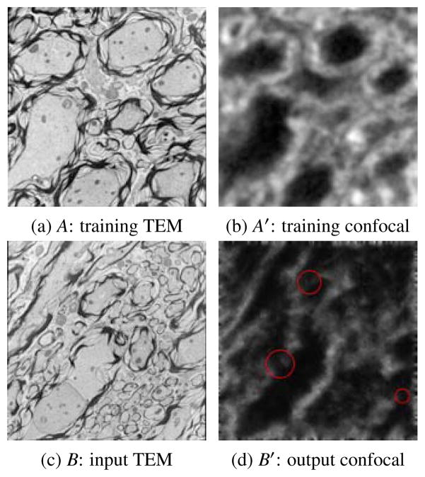
Image analogies, first introduced in (Hertzmann et al., 2001), have been widely used in texture synthesis. In this method, a pair of images A and A′ are provided as training data, where A′ is a “filtered” version of A. The “filter” is learned from A and A′ and is later applied to a different image B in order to generate an “analogous” filtered image. Fig. 2 shows an example of image analogies.

Figure 2.

Result of Image Analogies: Based on a training set (A, A′) an input image B can be transformed to B′ which mimics A′ in appearance. The red circles in (d) show inconsistent regions.

For multi-modal image registration, this method can be used to transfer a given image from one modality to another using the trained “filter”. Then the multi-modal image registration problem simplifies to a mono-modal one. However, since this method uses a nearest neighbor (NN) search of the image patch centered at each pixel, the resulting images are usually noisy because the L₂ norm based NN search does not preserve the local consistency well (see Fig. 2 (d)) (Hertzmann et al., 2001). This problem can be partially solved by a multi-scale search and a coherence search which enforce local consistency among neighboring pixels, but an effective solution is still missing. We introduce a sparse representation model to address this problem.

Sparse representation is a powerful model for representing and compressing high-dimensional signals (Wright et al., 2010; Huang et al., 2011b). It represents the signal with sparse combinations of some fixed bases which usually are not orthogonal to each other and are overcomplete to ensure its reconstruction power (Elad et al., 2010). It has been successfully applied many computer vision applications such as object recognition and classification in (Wright et al., 2009; Huang and Aviyente, 2007; Huang et al., 2011a; Zhang et al., 2012a, b; Fang et al., 2013; Cao et al., 2013). (Yang et al., 2010) also applied sparse representation to super resolution which is similar to our method. The differences between sparse representation based super resolution and image analogies are reconstruction constraints and the used data. In super resolution, the reconstruction constraint is between two images with different resolutions (the original low resolution image and predicted high resolution image). In order to make these two images comparable, additional blurring and downsampling operators are applied to the high resolution image, while in our method, we can direct compute the reconstruction error from the original image and reconstructed image from the sparse representation. Efficient algorithms based on convex optimization or greedy pursuit are available for computing sparse representations (Bruckstein et al., 2009).

The contribution of this paper is two-fold. First, we introduce a sparse representation model for image analogies which aims at improving the generalization ability and estimation result. Second, we simplify multi-modal image registration by using the image analogy approach to convert the registration problem to a mono-modal registration problem. The original idea in this paper was published in WBIR 2012 (Cao et al., 2012). This paper provides additional experiments, details of our method, and a more extensive review of related work. The flowchart of our method is shown in Fig. 3.

Figure 3.

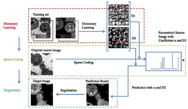
Flowchart of our proposed method. This method has three components: 1. dictionary learning: learning multi-modal dictionaries for both training images from different modalities; 2. sparse coding: computing sparse coefficients for the learned dictionaries to reconstruct the source image while at the same time using the same coefficients to transfer the source image to another modality; 3. registration: registering both transferred source image and target image.

3. Method

3.1. Standard Image Analogies

The objective for image analogies is to create an image B′ from an image B with a similar relation in appearance as a training image set (A, A′) (Hertzmann et al., 2001). The standard image analogies algorithm achieves the mapping between B and B′ by looking up best-matching patches for each image location between A and B which then imply the patch appearance for B′ from the corresponding patch A′ (A and A′ are assumed to be aligned). These best patches are smoothly combined to generate the overall output image B′. The algorithm description is presented in Alg. 1. To avoid costly lookups and to obtain a more generalizable model with noise-reducing properties we propose a sparse coding image analogies approach.

Algorithm 1.

Image Analogies.

Input:
	Training images: A and A′;
	Source image: B.
Output:
	’Filtered’ source B′.
1:	Construct Gaussian pyramids for A, A′ and B;
2:	Generate features for A, A′ and B;
3:	for each level l starting from coarsest do
4:	for each pixel $q\in B_l^{\prime }$, in scan-line order do
5:	Find best matching pixel p of q in Al and $A_l^{\prime }$;
6:	Assign the value of pixel p in A′ to the value of pixel q in $B_l^{\prime }$;
7:	Record the position of p.
8:	end for
9:	end for
10:	Return $B_L^{\prime }$ where L is the finest level.

3.2. Sparse Representation Model

Sparse representation is a technique to reconstruct a signal as a linear combination of a few basis signals from a typically over-complete dictionary. A dictionary is a collection of basis signals. The number of dictionary elements in an over-complete dictionary exceeds the dimension of the signal space (here the dimension of an image patch). Suppose a dictionary D is pre-defined. To sparsely represent a signal x the following optimization problem is solved (Elad, 2010):

$$\widehat{\alpha }=arg\underset{\alpha }{min}{\Vert \alpha \Vert }_0,\mathrm{s}.\mathrm{t}.{\Vert x-D\alpha \Vert }_2\le \epsilon ,$$ (1)

where α is a sparse vector that explains x as a linear combination of columns in dictionary D with error ε and || · ||₀ indicates the number of non-zero elements in the vector α. Solving (1) is an NP-hard problem. One possible solution of this problem is based on a relaxation that replaces || · ||₀ by || · ||₁, where || · ||₁ is the 1-norm of a vector, resulting in the optimization problem,

$$\widehat{\alpha }=arg\underset{\alpha }{min}{\Vert \alpha \Vert }_1,\mathrm{s}.\mathrm{t}.{\Vert x-D\alpha \Vert }_2\le \epsilon .$$ (2)

The equivalent Lagrangian form of (2) is

$$\widehat{\alpha }=arg\underset{\alpha }{min}\lambda {\Vert \alpha \Vert }_1+{\Vert x-D\alpha \Vert }_2^2,$$ (3)

which is a convex optimization problem that can be solved efficiently (Bruckstein et al., 2009; Boyd et al., 2010; Lee et al., 2006; Mairal et al., 2009).

A more general sparse representation model optimizes both α and the dictionary D,

$$\{\widehat{\alpha },\widehat{D}\}=arg\underset{\alpha ,D}{min}\lambda {\Vert \alpha \Vert }_1+{\Vert x-D\alpha \Vert }_2^2.$$ (4)

The optimization problem (3) is a sparse coding problem which finds the sparse codes α to represent x. Generating the dictionary D from a training dataset is called dictionary learning.

3.3. Image Analogies with Sparse Representation Model

For the registration of correlative microscopy images, given two training images A and A′ from different modalities, we can transform image B to the other modality by synthesizing B′. This idea is also applied to image colorization and demosaicing in (Mairal et al., 2007). Consider the sparse dictionary-based image denoising/reconstruction, u, given by minimizing

$$E(u,\{{\alpha }_i\})=\frac{\gamma }{2}{\Vert Lu-f\Vert }_2^2+\frac{1}{2}\sum _{i=1}^N{\Vert R_{i}u-D{\alpha }_i\Vert }_V^2+\lambda {\Vert {\alpha }_i\Vert }_1,$$ (5)

where f is the given (potentially noisy) image, D is the dictionary, {α_i} are the patch coefficients, R_i selects the i-th patch from the image reconstruction u, γ, λ > 0 are balancing constants, L is a linear operator (e.g., describing a convolution), and the norm is defined as ${\Vert x\Vert }_v^2=x^{T}Vx$, where V > 0 is positive definite. We jointly optimize for the coefficients and the reconstructed/denoised image. Formulation (5) can be extended to images analogies by minimizing

$$E(u^{(1)},u^{(2)},\{{\alpha }_i\})=\frac{\gamma }{2}{\Vert L^{(1)}{u}^{(1)}-f^{(1)}\Vert }_2^2+\frac{1}{2}\sum _{i=1}^N{\Vert R_i\left(\begin{array}{c}{u}^{(1)}\\ u^{(2)}\end{array}\right)-\left(\begin{array}{c}{D}^{(1)}\\ D^{(2)}\end{array}\right){\alpha }_i\Vert }_V^2+\lambda {\Vert {\alpha }_i\Vert }_1,$$ (6)

where we have corresponding dictionaries {D⁽¹⁾, D⁽²⁾} and only one image f⁽¹⁾ is given and we are seeking a reconstruction of a denoised version of f⁽¹⁾, u⁽¹⁾, as well as the corresponding analogous denoised image u⁽²⁾ (without the knowledge of f⁽²⁾). Note that there is only one set of coefficients α_i per patch, which indirectly relates the two reconstructions. The problem is convex (for given D⁽ⁱ⁾) which allows to compute a globally optimal solution. Section 3.5 describes our numerical solution approach.

Patch-based (non-sparse) denoising has also been proposed for the denoising of fluorescence microscopy images (Boulanger et al., 2010). A conceptually similar approach using sparse coding and image patch transfer has been proposed to relate different magnetic resonance images in (Roy et al., 2011). However, this approach does not address dictionary learning or spatial consistency considered in the sparse coding stage. Our approach addresses both and learns the dictionaries D⁽¹⁾ and D⁽²⁾ explicitly.

3.4. Dictionary Learning

Given sets of training patches { $p_i^{(1)},p_i^{(2)}$} We want to estimate the dictionaries themselves as well as the coefficients {α_i} for the sparse coding. The problem is non-convex (bilinear in D and α_i). The standard solution approach (Elad, 2010) is alternating minimization, i.e., solving for α_i keeping {D⁽¹⁾, D⁽²⁾} fixed and vice versa. Two cases need to be distinguished: (i) L locally invertible (or the identity) and (ii) L not locally-invertible (e.g., blurring due to convolution for a signal with the point spread function of a microscope). In the former case we can assume that the training patches are unrelated patches and we can compute local patch estimates { $p_i^{(1)},p_i^{(2)}$}directly by locally inverting the operator L for the given measurement {f⁽¹⁾, f⁽²⁾} for each patch. In the latter case, we need to consider patch size (for example for convolution) and can therefore not easily be inverted patch by patch. The non-local case is significantly more complicated, because the dictionary learning step needs to consider spatial dependencies between patches.

We only consider local dictionary learning here with L and V set to identities¹. We assume that the training patches $\{p_i^{(1)},p_i^{(2)}\}=\{f_i^{(1)},f_i^{(2)}\}$ are unrelated patches. Then the dictionary learning problem decouples from the image reconstruction and requires minimization of

$$\begin{array}{l}E(D,\{{\alpha }_i\})=\frac{1}{N}\sum _{i=1}^N\frac{1}{2}{\Vert \left(\begin{array}{c}{p}_i^{(1)}\\ p_i^{(2)}\end{array}\right)-\left(\begin{array}{c}{D}^{(1)}\\ D^{(2)}\end{array}\right){\alpha }_i\Vert }_2^2+\lambda {\Vert {\alpha }_i\Vert }_1\\ =\frac{1}{N}\sum _{i=1}^N\frac{1}{2}{\Vert p_i-D{\alpha }_i\Vert }_2^2+\lambda {\Vert {\alpha }_i\Vert }_1.\end{array}$$ (7)

The image analogy dictionary learning problem is identical to the one for image denoising. The only difference is a change in dimension for the dictionary and the patches (which are stacked up for the corresponding image sets). Usually to avoid D being arbitrarily large, a common constraint is added to each column of D where the l₂ norm of each column in D is less than or equal to one, i.e. $d_j^T{d}_j\le 1$, j = 1, …, m, D = {d₁, d₂, …, d_m} ∈ ℝ^nxm. Similar to (6), we use a single α in (7) to enforce the correspondence of the dictionaries between two modalities.

3.5. Numerical Solution

To simplify the optimization process of (6), we apply an alternating optimization approach (Elad, 2010) which initializes u⁽¹⁾ = f⁽¹⁾ and u⁽²⁾ = D⁽²⁾α at the beginning, and then computes the optimal α (the dictionary D⁽¹⁾ and D⁽²⁾ are assumed known here). Thus the minimization problem breaks into many smaller subparts, for each subproblem we have,

$$\widehat{\alpha }=arg\underset{\alpha }{min}\frac{1}{2}{\Vert R_i{u}^{(1)}-D^{(1)}{\alpha }_i\Vert }_2^2+\lambda {\Vert {\alpha }_i\Vert }_1,i\in 1,\dots N.$$ (8)

Following (Li and Osher, 2009) we use a coordinate descent algorithm to solve (8).

Given A = D⁽¹⁾, x = α_i and b = R_iu⁽¹⁾, then (8) can be rewritten in the general form

$$\widehat{x}=arg\underset{x}{min}\frac{1}{2}{\Vert b-Ax\Vert }_2^2+\lambda {\Vert x\Vert }_1.$$ (9)

The coordinate descent algorithm to solve (9) is described in Alg. 2. This algorithm minimizes (9) with respect to one component of x in one step, keeping all other components constant. This step is repeated until convergence.

Algorithm 2.

Coordinate Descent

Input: x = 0, λ > 0, β = ATb

Output: x

while not converged do

x̃ = Sλ (β)1; j = arg maxi |xi − x̃i|, where i is the index of the component in x and x̃; $x_i^{k+1}=x_i^k$, i ≠ j, and $x_j^{k+1}={\stackrel{\sim }{x}}_j$; ${\beta }^{k+1}={\beta }^k-\mid x_j^k-{\stackrel{\sim }{x}}_j\mid {(A^{T}A)}_j$, and ${\beta }_j^{k+1}={\beta }_j^k$, where (AT A)j is the jth column of (AT A).

end while

After solving (8), we can fix α and then update u⁽¹⁾. Now the optimization of (6) can be changed to

$${\widehat{u}}^{(1)}=arg\underset{u^{(1)}}{min}\frac{\gamma }{2}{\Vert u^{(1)}-f^{(1)}\Vert }_2^2+\sum _{i=1}^N\frac{1}{2}{\Vert R_i{u}^{(1)}-D^{(1)}{\alpha }_i\Vert }_2^2.$$ (10)

The closed-form solution of (10) is as follows²,

$${\widehat{u}}^{(1)}={(\gamma I+\sum _{i=1}^N{R}_i^T{R}_i)}^{-1}(\gamma f^{(1)}+\sum _{i=1}^N{R}_i^T{D}^{(1)}{\alpha }_i).$$ (11)

We iterate the optimization with respect to u⁽¹⁾ and α to convergence. Then u⁽²⁾ = D⁽²⁾α̂.

3.5.1. Dictionary Learning

We use a dictionary based approach and hence need to be able to learn a suitable dictionary from the data. We use alternating optimization. Assuming that the coefficients α_i and the measured patches { $p_i^{(1)},p_i^{(2)}$} are given, we compute the current best least-squares solution for the dictionary as ³

$$D=(\sum _{i=1}^N{p}_i{\alpha }_i^T){(\sum _{i=1}^N{\alpha }_i{\alpha }_i^T)}^{-1}.$$ (12)

The columns are normalized according to

$$d_j=d_j/max({\Vert d_j\Vert }_2,1),j=1,\dots ,m,$$ (13)

where D = {d₁,d₂, … d_m} ∈ ℝ^nxm. The optimization with respect to the α_i terms follows (for each patch independently) the coordinate descent algorithm. Since the local dictionary learning approach assumes that patches to learn the dictionary from are given, the problem completely decouples with respect to the coefficients α_i and we obtain

$$E=\frac{1}{N}\sum _{i=1}^N\frac{1}{2}{\Vert p_i-D{\alpha }_i\Vert }_2^2+\lambda {\Vert {\alpha }_i\Vert }_1$$ (14)

where $p_i=\{p_i^{(1)},p_i^{(2)}\}$ and D = {D⁽¹⁾,D⁽²⁾}.

3.6. Intensity Normalization

The image analogy approach may not be able to achieve a perfect prediction because: a) image intensities are normalized and hence the original dynamic range of the images is not preserved and b) image contrast may be lost as the reconstruction is based on the weighted averaging of patches. To reduce the intensity distribution discrepancy between the predicted image and original image, in our method, we apply intensity normalization (normalize the different dynamic ranges of different images to the same scale for example [0,1]) to the training images before dictionary learning, and also to the image analogy results.

3.7. Use in Image Registration

For image registration, we (i) reconstruct the “missing” analogous image and (ii) consistently denoise the given image to be registered with (Elad and Aharon, 2006). By denoising the target image using the learned dictionary for the target image from the joint dictionary learning step we obtain two consistently denoised images: the denoised target image and the predicted source image. The image registration is applied to the analogous image and the target image. We consider rigid followed by affine and B-spline registrations in this paper and use elastix’s implementation (Klein et al., 2010; Ibanez et al., 2005). As similarity measures we use sum of squared differences (SSD) and mutual information (MI). A standard gradient descent is used for optimization. For B-spline registration, we use displacement magnitude regularization which penalizes ||T(x) − x||², where T(x) is the transformation of coordinate x in an image (Klein et al., 2010). This is justified as we do not expect large deformations between the images as they represent the same structure. Hence, small displacements are expected, which are favored by this form of regularization.

4. Results

4.1. Data

We use both 2D correlative SEM/confocal images with fiducials and TEM/confocal images of mouse brains in our experiment. All the experiments are performed on a Dell OptiPlex 980 computer with an Intel Core i7 860 2.9GHz CPU. The data description is shown in Tab. 1.

Table 1.

Data Description

	Data Types
	SEM/confocal	TEM/confocal
Number of datasets	8	6
Fiducial	100 nm gold	none
Pixel Size	40 nm	0.069μm

4.2. Registration of SEM/confocal images (with fiducials)

4.2.1. Pre-processing

The confocal images are denoised by the sparse representation-based denoising method (Elad, 2010). We use a landmark based registration on the fiducials to obtain the gold standard alignment results. The image size is about 400 ×400 pixels.

4.2.2. Image Analogies (IA) Results

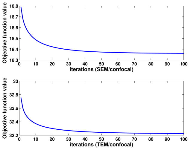
We applied the standard IA method and our proposed method. We trained the dictionaries using a leave-one-out approach. The training image patches are extracted from pre-registered SEM/confocal images as part of the preprocessing described in Section 4.2.1. In both IA methods we use 10 × 10 patches, and in our proposed method we randomly sample 50000 patches and learn 1000 dictionary elements in the dictionary learning phase. The learned dictionaries are shown in Fig. 5. We choose γ = 1 and λ = 0.15 in (6). In Fig. 8, both IA methods can reconstruct the confocal image very well but our proposed method preserves more structure than the standard IA method. We also show the prediction errors and the statistical scores of our proposed IA method and standard IA method for SEM/confocal images in Tab. 2. The prediction error is defined as the sum of squared intensity differences between the predicted confocal image and the original confocal image. Our method is based on patch-by-patch prediction using the learned multi-modal dictionary. Given a particular patch-size the number of sparse coding problems in our model changes linearly with the number of pixels in an image. Our method is much faster than the standard image analogies method which involves an exhaustive search of the whole training set as our method is based on a dictionary representation. For example, our method takes about 500 secs for a 1024×1024 image with image patch size 10×10 and dictionary size 1000 while the standard image analogy method takes more than 30 mins for the same patch size. The CPU processing time for SEM/confocal data is shown in Tab. 3. We also illustrate the convergence of solving (14) for both SEM/confocal and TEM/confocal images in Fig. 7 which shows that 100 iterations are sufficient for both datasets..

Figure 5.

Results of dictionary learning: the left dictionary is learned from the SEM and the corresponding right dictionary is learned from the confocal image.

Figure 8.

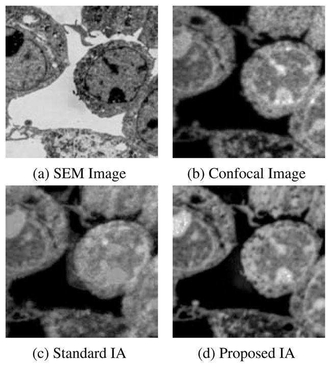
Results of estimating a confocal (b) from an SEM image (a) using the standard IA (c) and our proposed IA method (d).

Table 2.

Prediction results for SEM/confocal images. Prediction is based on the proposed IA and standard IA methods, and we use sum of squared prediction residuals (SSR) to evaluate the prediction results. The p-value is computed using a paired t-test.

Method	mean	std	p-value
Proposed IA	1.52 ×105	5.79 ×104	0.0002
Standard IA	2.83 ×105	7.11 ×104

Table 3.

CPU time (in seconds) for SEM/confocal images. The p-value is computed using a paired t-test.

Method	mean	std	p-value
Proposed IA	82.2	6.7	0.00006
Standard IA	407.3	10.1

Figure 7.

Convergence test on SEM/confocal and TEM/confocal images. The objective function is defined as in (14). The maximum iteration number is 100. The patch size for SEM/confocal images and TEM/confocal images are 10 ×10 and 15 ×15 respectively.

4.2.3. Image Registration Results

We resampled the estimated confocal images with up to ±600 nm (15 pixels) in translation in the x and y directions (at steps of 5 pixel) and ±15° in rotation (at steps of 5 degree) with respect to the gold standard alignment. Then we registered the resampled estimated confocal images to the corresponding original confocal images. The goal of this experiment is to test the ability of our methods to recover from misalignments by translating and rotating the pre-aligned image within a practically reasonable range. Such a rough initial automatic alignment can for example be achieved by image correlation. The image registration results based on both image analogy methods are compared to registration results using original images using both SSD and MI as similarity measures¹. Tab. 4 summarizes the registration results on translation and rotation errors based on the rigid transformation model for each image pair over all these experiments. The results are reported as physical distances instead of pixels. We also perform registrations using affine and B-spline transformation models. These registrations are initialized with the result from the rigid registration. Fig. 6 shows the box plot for all the registration results.

Table 4.

SEM/confocal rigid registration errors on translation (t) and rotation (r)( $t=\sqrt{t_x^2+t_y^2}$ where t_x and t_y are translation errors in x and y directions respectively; t is in nm; pixel size is 40nm; r is in degree.) Here, the registration methods include: Original Image SSD and Original Image MI, registrations with original images based on SSD and MI metrics respectively; Standard IA SSD and Standard IA MI, registration with standard IA algorithm based on SSD and MI metrics respectively; Proposed IA SSD and Proposed IA MI, registration with our proposed IA algorithm based on SSD and MI metrics respectively.

	rmean	rmedian	rstd	tmean	tmedian	tstd
Proposed IA SSD	0.357	0.255	0.226	92.457	91.940	56.178
Proposed IA MI	0.239	0.227	0.077	83.299	81.526	54.310
Standard IA SSD	0.377	0.319	0.215	178.782	104.362	162.266
Standard IA MI	0.3396	0.332	0.133	140.401	82.667	135.065
Original Image SSD	0.635	0.571	0.215	170.484	110.317	117.371
Original Image MI	0.516	0.423	0.320	176.203	104.574	116.290

Figure 6.

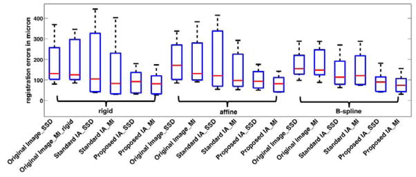
Box plot for the registration results of SEM/confocal images on landmark errors of different methods with three transformation models: rigid, affine and B-spline. The registration methods include: Original Image SSD and Original Image MI, registrations with original images based on SSD and MI metrics respectively; Standard IA SSD and Standard IA MI, registration with standard IA algorithm based on SSD and MI metrics respectively; Proposed IA SSD and Proposed IA MI, registration with our proposed IA algorithm based on SSD and MI metrics respectively. The bottom and top edges of the boxes are the 25th and 75th percentiles, the central red lines are the medians.

4.2.4. Hypothesis Test on Registration Results

In order to check whether the registration results from different methods are statistically different with each other, we use hypothesis testing (Weiss and Weiss, 2012). We assume the registration results (rotations and translations) are independent and normally distributed random variables with means μ_i and variances ${\sigma }_i^2$. For the results from 2 different methods, the null hypothesis (H₀) is μ₁ = μ₂, and the alternative hypothesis (H₁) is μ₁ ≤ μ₂. We apply the one-sided paired sample t-test for equal means using MATLAB (MATLAB, 2012). The level of significance is set at 5%. Based on the hypothesis test results in Tab. 5, our proposed method shows significant differences with respect to the standard IA method for the registration error with respect to the SSD metric on rigid registration and both MI and SSD metrics for affine and B-spline registrations. Tables 4 and 5 also show that our method outperforms the standard image analogy method as well as the direct use of mutual information on the original images in terms of registration accuracy. However, as deformations are generally relatively rigid no statistically significant improvements in registration results could be found within a given method relative to the different transformation models as illustrated in Tab. 6.

Table 5.

Hypothesis test results (p-values) with multiple testing correction results (FDR corrected p-values in parentheses) for registration results evaluated via landmark errors for SEM/confocal images. We use a one-sided paired t-test. Comparison of different image types (original image, standard IA, proposed IA) using the same registration models (rigid, affine, B-spline). The proposed model shows the best performance for all transformation models. (Bold indicates statistically significant improvement at significance level α = 0.05 after correcting for multiple comparisons with FDR (Benjamini and Hochberg, 1995).)

		Original Image/Standard IA	Original Image/Proposed IA	Standard IA/Proposed IA
Rigid	SSD	0.5017 (0.5236)	0.0040 (0.0102)	0.0482 (0.0668)
	MI	0.0747 (0.0961)	0.0014 (0.0052)	0.0888(0.1065)
Affine	SSD	0.5236 (0.5236)	0.0013 (0.0052)	0.0357 (0.0535)
	MI	0.0298 (0.0488)	0.0048 (0.0108)	0.0258 (0.0465)
B-spline	SSD	0.0017 (0.0052)	0.0001 (0.0023)	0.0089 (0.0179)
	MI	0.1491 (0.1678)	0.0002 (0.0024)	0.0017 (0.0052)

Table 6.

Hypothesis test results (p-values) with multiple testing correction results (FDR corrected p-values in parentheses) for registration results measured via landmark errors for SEM/confocal images. We use a one-sided paired t-test. Comparison of different registration models (rigid, affine, B-spline) within the same image types (original image, standard IA, proposed IA). Results are not statistically significantly better after correcting for multiple comparisons with FDR.)

		Rigid/Affine	Rigid/B-spline	Affine/B-spline
Original Image	SSD	0.7918 (0.8908)	0.3974 (0.6596)	0.1631 (0.5873)
	MI	0.6122 (0.7952)	0.3902 (0.6596)	0.3635 (0.6596)
Standard IA	SSD	0.9181 (0.9371)	0.1593 (0.5873)	0.0726 (0.5873)
	MI	0.5043 (0.7564)	0.6185 (0.7952)	0.7459 (0.8908)
Proposed IA	SSD	0.9371 (0.9371)	0.3742 (0.6596)	0.0448 (0.5873)
	MI	0.4031 (0.6596)	0.1616 (0.5873)	0.2726 (0.6596)

4.2.5. Discussion

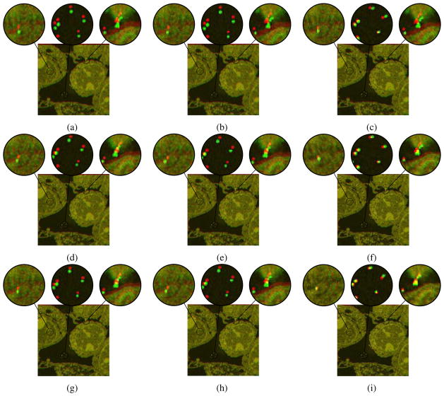
From Fig. 6, the improvement of registration results from rigid registration to affine and B-spline registrations are not significant due to the fact that both SEM/-confocal images are acquired from the same piece of tissue section. The rigid transformation model can capture the deformation well enough, though small improvements can visually be observed using more flexible transformation models as illustrated in the composition images between the registered SEM images using three registration methods (direct registration and the two IA methods) and the registered SEM images based on fiducials of Fig. 9. Our proposed method can achieve the best results for all the three registration models. See also Tab. 6.

Figure 9.

Results of registration for SEM/confocal images using MI similarity measure with direct registration (first row), standard IA (second row) and our proposed IA method (third row) for (a, d, g) rigid registration (b, e, h) affine registration and (c, f, i) b-spline registration. Some regions are zoomed in to highlight the distances between corresponding fiducials. The images show the compositions of the registered SEM images using the three registration methods (direct registration, standard IA and proposed IA methods) and the registered SEM image based on fiducials respectively. Differences are generally very small indicating that for these images a rigid transformation model may already be sufficiently good.

4.3. Registration of TEM/confocal images (without fiducials)

4.3.1. Pre-processing

We extract the corresponding region of the confocal image and resample both confocal and TEM images to an intermediate resolution. The final resolution is 14.52 pixels per μm, and the image size is about 256×256 pixels. The datasets are already roughly registered based on manually labeled landmarks with a rigid transformation model.

4.3.2. Image Analogies Results

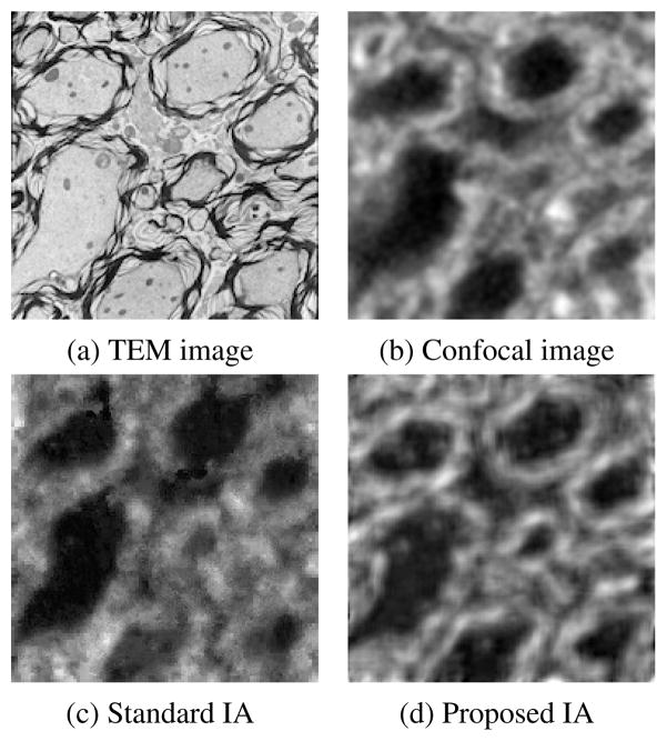
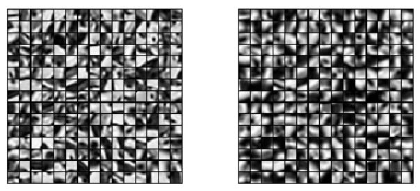
We tested the standard image analogy method and our proposed sparse method. For both image analogy methods we use 15 ×15 patches, and for our method we randomly sample 50000 patches and learn 1000 dictionary elements in the dictionary learning phase. The learned dictionaries are shown in Fig. 11. We choose γ = 1 and λ = 0.1 in (6). The image analogies results in Fig. 12 show that our proposed method preserves more local structure than the standard image analogy method. We show the prediction error of our proposed IA method and standard IA method for TEM/confocal images in Tab. 7. The CPU processing time for the TEM/confocal data is given in Tab. 8.

Figure 11.

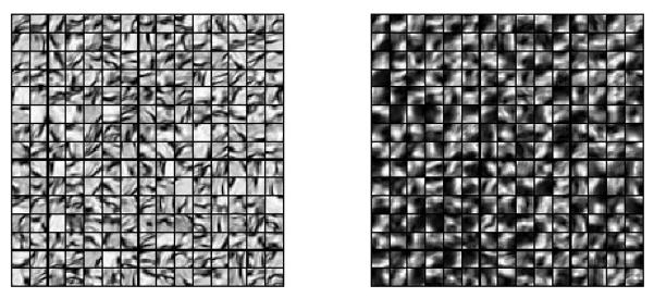
Results of dictionary learning: the left dictionary is learned from the TEM and the corresponding right dictionary is learned from the confocal image.

Figure 12.

Result of estimating the confocal image (b) from the TEM image (a) for the standard image analogy method (c) and the proposed sparse image analogy method (d) which shows better preservation of structure.

Table 7.

Prediction results for TEM/confocal images. Prediction is based on the proposed IA and standard IA methods, and we use SSR to evaluate the prediction results. The p-value is computed using a paired t-test.

Method	mean	std	p-value
Proposed IA	7.43 ×104	4.72 ×103	0.0015
Standard IA	8.62 ×104	6.37 ×103

Table 8.

CPU time (in seconds) for TEM/confocal images. The p-value is computed using a paired t-test.

Method	mean	std	p-value
Proposed IA	35.2	4.4	0.00019
Standard IA	196.4	8.1

4.3.3. Image Registration Results

We manually determined 10 ~ 15 corresponding landmark pairs on each dataset to establish a gold standard for registration. The same type and magnitude of shifts and rotations as for the SEM/confocal experiment are applied. The image registration results based on both image analogy methods are compared to the landmark based image registration results using mean absolute errors (MAE) and standard deviations (STD) of the absolute errors on all the corresponding landmarks. We use both SSD and mutual information (MI) as similarity measures. The registration results are displayed in Fig. 14 and Table 9. The landmark based image registration result is the best result achievable given the affine transformation model. We show the results for both image analogy methods as well as using the original TEM/confocal image pairs¹. Fig. 14 shows that the MI based image registration results are similar among the three methods and our proposed method performs slightly better. The results are reported as physical distances instead of pixels. Also the results of our method are close to the landmark based registration results (best registration results). For SSD based image registration, our proposed method is more robust than the other two methods for the current dataset.

Figure 14.

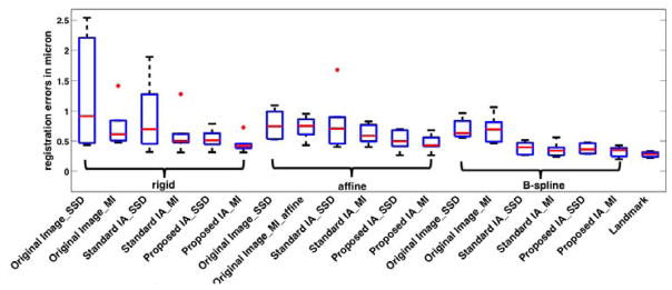
Box plot for the registration results of TEM/confocal images for different methods. The bottom and top edges of the boxes are 25th and 75th percentiles, the central red lines indicate the medians.

Table 9.

TEM/confocal rigid registration results (in μm, pixel size is 0.069 μm).

		Proposed IA		Standard IA		Original Image		Landmark
case		MAE	STD	MAE	STD	MAE	STD	MAE	STD
1	SSD	0.3174	0.2698	0.3219	0.2622	0.4352	0.2519	0.2705	0.1835
	MI	0.3146	0.2657	0.3132	0.2601	0.5161	0.2270
2	SSD	0.4911	0.1642	0.5759	0.2160	2.5420	1.6877	0.3091	0.1594
	MI	0.4473	0.1869	0.4747	0.3567	1.4245	0.1780
3	SSD	0.5379	0.2291	1.8940	1.0447	0.5067	0.2318	0.3636	0.1746
	MI	0.3864	0.2649	0.5261	0.2008	0.4078	0.2608
4	SSD	0.4451	0.2194	0.4516	0.2215	0.4671	0.2484	0.3823	0.2049
	MI	0.4554	0.2298	0.4250	0.2408	0.4740	0.2374
5	SSD	0.6268	0.2505	1.2724	0.6734	1.3174	0.3899	0.2898	0.2008
	MI	0.3843	0.2346	0.6172	0.2429	0.7018	0.2519
6	SSD	0.7832	0.5575	0.8159	0.4975	2.2080	1.4228	0.3643	0.1435
	MI	0.7259	0.4809	1.2772	0.4285	0.8383	0.4430

4.3.4. Hypothesis Test on Registration Results

We use the same hypothesis test method as in Section 4.2.4, and test the means of different methods on MAE of corresponding landmarks. Table 10 and 11 indicate that the registration result of our proposed method shows significant improvement over the result using original images with both SSD and MI metric. Also, the result of our proposed method is significantly better than the standard IA method with MI metric.

Table 10.

Hypothesis test results (p-values) with multiple testing correction results (FDR corrected p-values in parentheses) for registration results measured via landmark errors for TEM/confocal images. We use a one-sided paired t-test. Comparison of different image types (original image, standard IA, proposed IA) using the same registration models (rigid, affine, B-spline). The proposed image analogy method performs better for affine and B-spline deformation models. (Bold indicates statistically significant improvement at a significance level α = 0.05 after correcting for multiple comparisons with FDR.)

		Original Image/Standard IA	Original Image/Proposed IA	Standard IA/Proposed IA
Rigid	SSD	0.2458 (0.2919)	0.0488 (0.1069)	0.0869 (0.1303)
	MI	0.2594 (0.2919)	0.0478 (0.1069)	0.0594 (0.1069)
Affine	SSD	0.5864 (0.5864)	0.0148 (0.0445)	0.0750 (0.1226)
	MI	0.1593 (0.2048)	0.0137 (0.0445)	0.0556 (0.1069)
B-spline	SSD	0.0083 (0.0445)	0.0085 (0.0445)	0.3597 (0.3809)
	MI	0.0148 (0.0445)	0.0054 (0.0445)	0.1164 (0.1611)

Table 11.

Hypothesis test results (p-values) with multiple testing correction results (FDR corrected p-values in parentheses) for registration results evaluated via landmark errors for TEM/confocal images. We use a one-sided paired t-test. Comparison of different image types (original image, standard IA, proposed IA) using the same registration models (rigid, affine, B-spline). Results are overall suggestive of the benefit of B-spline registration, but except for the standard IA do not reach significance after correction for multiple comparisons. This may be due to the limited sample size. (Bold indicates statistically significant improvement after correcting for multiple comparisons with FDR.)

		Rigid/Affine	Rigid/B-spline	Affine/B-spline
Original Image	SSD	0.0792(0.1583)	0.1149(0.2069)	0.3058(0.4865)
	MI	0.4325(0.4865)	0.4091(0.4865)	0.3996(0.4865)
Standard IA	SSD	0.3818(0.4865)	0.0289(0.1041)	0.0280(0.1041)
	MI	0.4899(0.5188)	0.0742(0.1583)	0.0009(0.0177)
Proposed IA	SSD	0.3823(0.4865)	0.0365(0.1096)	0.0216(0.1041)
	MI	0.5431(0.5431)	0.0595(0.1531)	0.0150(0.1041)

4.3.5. Discussion

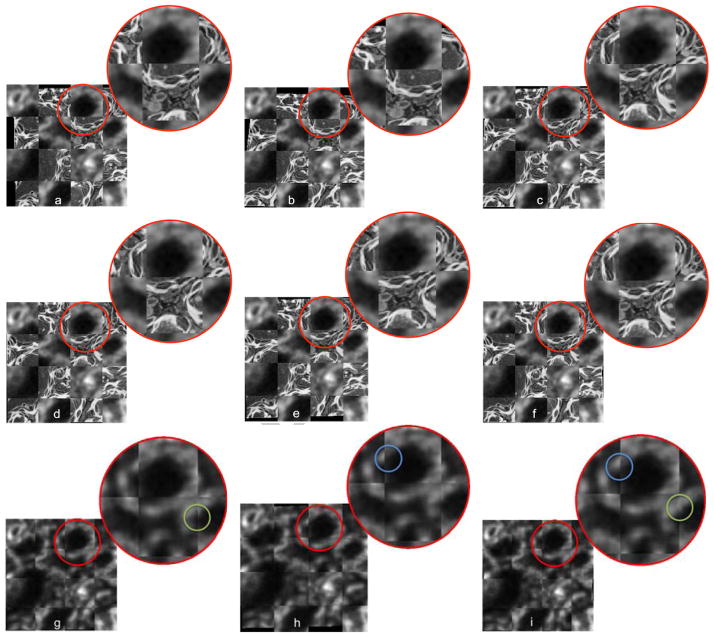
In Fig. 14, the affine and B-spline registrations using our proposed IA method show significant improvement compared with affine and B-spline registrations on the original images. In comparison to the SEM/confocal experiment (Fig. 9) the checkerboard image shown in Fig. 13 shows slightly stronger deformations for the more flexible B-spline model leading to slightly better local alignment. Our proposed method still achieves the best results for the three registration models.

Figure 13.

Results of registration for TEM/confocal images using MI similarity measure with directly registration (first row) and our proposed IA method (second and third rows) using (a, d, g) rigid registration (b, e, h) affine registration and (c, f, i) b-spline registration. The results are shown in a checkerboard image for comparison. Here, first and second rows show the checkerboard images of the original TEM/confocal images ¹ while the third row shows the checkerboard image of the results of our proposed IA method. Differences are generally small, but some improvements can be observed for B-spline registration.

¹The grayscale values of original TEM image are inverted for better visualization

5. Conclusion

We developed a multi-modal registration method for correlative microscopy. The method is based on image analogies with a sparse representation model. Our method can be regarded as learning a mapping between image modalities such that either an SSD or MI image similarity measure becomes appropriate for image registration. Any desired image registration model could be combined with our method as long as it supports either SSD or a MI as an image similarity measure. Our method then becomes an image pre-processing step. We tested our method on SEM/confocal and TEM/confocal image pairs with rigid registration followed by affine and B-spline registrations. The image registration results from Fig. 6, 14 suggest that the sparse image analogy method can improve registration robustness and accuracy. While our method does not show improvements for every individual dataset, our method improved registration results significantly for the SEM/-confocal experiments for all transformation models and for the TEM/confocal experiments for affine and B-spline registration. Furthermore, when using our image analogy method multi-modal registration based on SSD becomes feasible. We also compared the runtime between the standard IA and the proposed IA methods. Our proposed method runs about 5 times faster than the standard method. While the runtime is far from real-time performance, the method is sufficiently fast for correlative microscopy applications.

Our future work includes additional validation on a larger number of datasets from different modalities. Our goal is also to estimate the local quality of the image analogy result. This quality estimate could then be used to weight the registration similarity metrics to focus on regions of high confidence. Other similarity measures can be modulated similarly. We will also apply our sparse image analogy method to 3D images.

Figure 4.

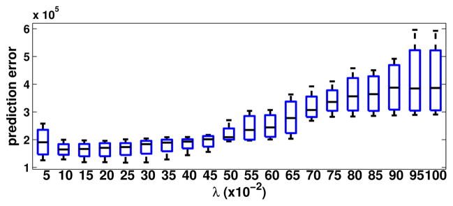
Prediction errors with respect to different λ values for SEM/-confocal image. The λ values are tested from 0.05–1.0 with step size 0.05.

Figure 10.

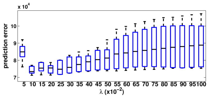
Prediction errors for different λ values for TEM/confocal image. The λ values are tested from 0.05–1.0 with step size 0.05.

Appendix A. Updating u⁽¹⁾ (reconstruction of f⁽¹⁾)

The sparse representation based image analogies method is defined as the minimization of

$$E(u^{(1)},u^{(2)},\{{\alpha }_i\})=\frac{\gamma }{2}{\Vert u^{(1)}-f^{(1)}\Vert }_2^2+\frac{1}{2}\sum _{i=1}^N{\Vert R_i\left(\begin{array}{c}{u}^{(1)}\\ u^{(2)}\end{array}\right)-\left(\begin{array}{c}{D}^{(1)}\\ D^{(2)}\end{array}\right){\alpha }_i\Vert }_2^2+\lambda {\Vert {\alpha }_i\Vert }_1.$$ (A.1)

We use an alternating optimization method to solve (A.1). Given a dictionary D⁽¹⁾ and corresponding coefficients α, we want to update u⁽¹⁾ by minimizing the following energy function

$$E_{D^{(1)},\alpha }(u^{(1)})=\frac{\gamma }{2}{\Vert u^{(1)}-f^{(1)}\Vert }_2^2+\frac{1}{2}\sum _{i=1}^N{\Vert R_i{u}^{(1)}-D^{(1)}{\alpha }_i\Vert }_2^2.$$

Differentiating the energy yields

$$\frac{\partial E}{\partial u^{(1)}}=\gamma (u^{(1)}-f^{(1)})+\sum _{i=1}^N{R}_i^T(R_i{u}^{(1)}-D^{(1)}{\alpha }_i)=0.$$

After rearranging, we get

$$u^{(1)}={(\gamma I+\sum _{i=1}^N{R}_i^T{R}_i)}^{-1}(\gamma f^{(1)}+\sum _{i=1}^N{R}_i^T{D}^{(1)}{\alpha }_i).$$

Appendix B. Updating the Dictionary

Assume we are given current patch estimates and dictionary coefficients. The patch estimates can be obtained from an underlying solution step for the non-local dictionary approach or given directly for local dictionary learning. The dictionary-dependent energy can be rewritten as

$$\begin{array}{l}{E}_d(D,\{{\alpha }_i\})=\sum _{i=1}^N\frac{1}{2}{(p_i-D{\alpha }_i)}^T(p_i-D{\alpha }_i)+\lambda {\Vert {\alpha }_i\Vert }_1\\ =\sum _{i=1}^N\frac{1}{2}(p_i^T{p}_i-p_i^{T}D{\alpha }_i-{\alpha }_i^T{D}^T{p}_i+{\alpha }_i^T{D}^{T}D{\alpha }_i)+\lambda {\Vert {\alpha }_i\Vert }_1.\end{array}$$

Using the derivation rules ((Petersen and Pedersen, 2008))

$$\frac{\partial a^{T}Xb}{\partial X}={ab}^T,\frac{\partial a^T{X}^{T}b}{\partial X}={ba}^T,\frac{b^T{X}^{T}Xc}{\partial X}={\mathit{Xbc}}^T+{\mathit{Xcb}}^T,$$

we obtain

$$\frac{\partial E_d(D,\{{\alpha }_i\})}{\partial D}=\sum _{i=1}^N(D{\alpha }_i-p_i){\alpha }_i^T=0.$$

After some rearranging, we obtain

$$D\underset{=A}{\underbrace{\sum _{i=1}^N{\alpha }_i{\alpha }_i^T}}=\underset{=B}{\underbrace{\sum _{i=1}^N{p}_i{\alpha }_i^T}}.$$

If A is invertible we obtain

$$D=(\sum _{i=1}^N{p}_i{\alpha }_i^T){(\sum _{i=1}^N{\alpha }_i{\alpha }_i^T)}^{-1}={BA}^{-1}.$$

References

- Benjamini Y, Hochberg Y. Controlling the false discovery rate: a practical and powerful approach to multiple testing. Journal of the Royal Statistical Society. Series B (Methodological) 1995:289–300. [Google Scholar]
- Boulanger J, Kervrann C, Bouthemy P, Elbau P, Sibarita J, Salamero J. Patch-based nonlocal functional for denoising fluorescence microscopy image sequences. Medical Imaging, IEEE Transactions on. 2010;29:442–454. doi: 10.1109/TMI.2009.2033991. [DOI] [PubMed] [Google Scholar]
- Boyd S, Parikh N, Chu E, Peleato B, Eckstein J. Distributed optimization and statistical learning via the alternating direction method of multipliers. Machine Learning. 2010;3:1–123. [Google Scholar]
- Bruckstein A, Donoho D, Elad M. From sparse solutions of systems of equations to sparse modeling of signals and images. SIAM review. 2009;51:34–81. [Google Scholar]
- Cao T, Jojic V, Modla S, Powell D, Czymmek K, Niethammer M. Robust multimodal dictionary learning, in: Medical Image Computing and Computer-Assisted Intervention–MICCAI 2013. Springer; Berlin Heidelberg: 2013. pp. 259–266. [DOI] [PMC free article] [PubMed] [Google Scholar]
- Cao T, Zach C, Modla S, Powell D, Czymmek K, Niethammer M. Registration for correlative microscopy using image analogies. Biomedical Image Registration. 2012:296–306. doi: 10.1016/j.media.2013.12.005. [DOI] [PMC free article] [PubMed] [Google Scholar]
- Caplan J, Niethammer M, Taylor R, II, Czymmek K. The power of correlative microscopy: multi-modal, multi-scale, multi-, dimensional. Current Opinion in Structural Biology. 2011 doi: 10.1016/j.sbi.2011.06.010. [DOI] [PMC free article] [PubMed] [Google Scholar]
- Elad M. Sparse and redundant representations: from theory to applications in signal and image processing. Springer Verlag; 2010. [Google Scholar]
- Elad M, Aharon M. Image denoising via sparse and redundant representations over learned dictionaries. Image Processing, IEEE Transactions on. 2006;15:3736–3745. doi: 10.1109/tip.2006.881969. [DOI] [PubMed] [Google Scholar]
- Elad M, Figueiredo M, Ma Y. On the role of sparse and redundant representations in image processing. Proceedings of the IEEE. 2010;98:972–982. [Google Scholar]
- Fang R, Chen T, Sanelli PC. Towards robust deconvolution of low-dose perfusion ct: Sparse perfusion deconvolution using online dictionary learning. Medical image analysis. 2013 doi: 10.1016/j.media.2013.02.005. [DOI] [PMC free article] [PubMed] [Google Scholar]
- Fronczek D, Quammen C, Wang H, Kisker C, Superfine R, Taylor R, Erie D, Tessmer I. High accuracy fiona-afm hybrid imaging. Ultramicroscopy. 2011 doi: 10.1016/j.ultramic.2011.01.020. [DOI] [PMC free article] [PubMed] [Google Scholar]
- Hertzmann A, Jacobs C, Oliver N, Curless B, Salesin D. Image analogies. Proceedings of the 28th annual conference on Computer graphics and interactive techniques; 2001. pp. 327–340. [Google Scholar]
- Huang J, Zhang S, Metaxas D. Efficient mr image reconstruction for compressed mr imaging. Medical Image Analysis. 2011a;15:670–679. doi: 10.1016/j.media.2011.06.001. [DOI] [PubMed] [Google Scholar]
- Huang J, Zhang T, Metaxas D. Learning with structured sparsity. The Journal of Machine Learning Research. 2011b;12:3371–3412. [Google Scholar]
- Huang K, Aviyente S. Sparse representation for signal classification. Advances in neural information processing systems. 2007;19:609. [Google Scholar]
- Ibanez L, Schroeder W, Ng L, Cates J. The ITK Software Guide. 2 Kitware, Inc; 2005. http://www.itk.org/ItkSoftwareGuide.pdf. [Google Scholar]
- Kaynig V, Fischer B, Wepf R, Buhmann J. Fully automatic registration of electron microscopy images with high and low resolution. Microsc Microanal. 2007;13:198–199. [Google Scholar]
- Klein S, Staring M, Murphy K, Viergever MA, Pluim JP, et al. Elastix: a toolbox for intensity-based medical image registration. IEEE transactions on medical imaging. 2010;29:196–205. doi: 10.1109/TMI.2009.2035616. [DOI] [PubMed] [Google Scholar]
- Lee H, Battle A, Raina R, Ng A. Efficient sparse coding algorithms. Advances in neural information processing systems. 2006:801–808. [Google Scholar]
- Li Y, Osher S. Coordinate descent optimization for 1 minimization with application to compressed sensing; a greedy algorithm. Inverse Probl Imaging. 2009;3:487–503. [Google Scholar]
- Mairal J, Bach F, Ponce J, Sapiro G. Online dictionary learning for sparse coding. Proceedings of the 26th Annual International Conference on Machine Learning; ACM; 2009. pp. 689–696. [Google Scholar]
- Mairal J, Mairal J, Elad M, Elad M, Sapiro G, Sapiro G. Sparse representation for color image restoration. the IEEE Trans. on Image Processing; ITIP; 2007. pp. 53–69. [DOI] [PubMed] [Google Scholar]
- MATLAB. version 7.14.0 (R201aa) The MathWorks Inc; Natick, Massachusetts: 2012. [Google Scholar]
- Petersen K, Pedersen M. The matrix cookbook. Technical University of Denmark; 2008. pp. 7–15. [Google Scholar]
- Roy S, Carass A, Prince J. Information Processing in Medical Imaging. Springer; 2011. A compressed sensing approach for mr tissue contrast synthesis; pp. 371–383. [DOI] [PMC free article] [PubMed] [Google Scholar]
- Wachinger C, Navab N. Manifold learning for multimodal image registration. 11st British Machine Vision Conference (BMVC).2010. [Google Scholar]
- Wein W, Brunke S, Khamene A, Callstrom MR, Navab N. Automatic ct-ultrasound registration for diagnostic imaging and image-guided intervention. Medical image analysis. 2008;12:577. doi: 10.1016/j.media.2008.06.006. [DOI] [PubMed] [Google Scholar]
- Weiss N, Weiss C. Introductory statistics. Addison-Wesley; 2012. [Google Scholar]
- Wells W, III, Viola P, Atsumi H, Nakajima S, Kikinis R. Multi-modal volume registration by maximization of mutual information. Medical image analysis. 1996;1:35–51. doi: 10.1016/s1361-8415(01)80004-9. [DOI] [PubMed] [Google Scholar]
- Wright J, Ma Y, Mairal J, Sapiro G, Huang T, Yan S. Sparse representation for computer vision and pattern recognition. Proceedings of the IEEE. 2010;98:1031–1044. [Google Scholar]
- Wright J, Yang A, Ganesh A, Sastry S, Ma Y. Robust face recognition via sparse representation. Pattern Analysis and Machine Intelligence, IEEE Transactions on. 2009;31:210–227. doi: 10.1109/TPAMI.2008.79. [DOI] [PubMed] [Google Scholar]
- Yang J, Wright J, Huang T, Ma Y. Image super-resolution via sparse representation. Image Processing, IEEE Transactions on. 2010;19:2861–2873. doi: 10.1109/TIP.2010.2050625. [DOI] [PubMed] [Google Scholar]
- Yang S, Kohler D, Teller K, Cremer T, Le Baccon P, Heard E, Eils R, Rohr K. Nonrigid registration of 3-d multichannel microscopy images of cell nuclei. Image Processing, IEEE Transactions on. 2008;17:493–499. doi: 10.1109/TIP.2008.918017. [DOI] [PubMed] [Google Scholar]
- Zhang S, Zhan Y, Dewan M, Huang J, Metaxas DN, Zhou XS. Towards robust and effective shape modeling: Sparse shape composition. Medical image analysis. 2012a;16:265–277. doi: 10.1016/j.media.2011.08.004. [DOI] [PubMed] [Google Scholar]
- Zhang S, Zhan Y, Metaxas DN. Deformable segmentation via sparse representation and dictionary learning. Medical Image Analysis. 2012b doi: 10.1016/j.media.2012.07.007. [DOI] [PubMed] [Google Scholar]