Self-organized noise resistance of oscillatory neural networks with spike timing-dependent plasticity

Abstract

Intuitively one might expect independent noise to be a powerful tool for desynchronizing a population of synchronized neurons. We here show that, intriguingly, for oscillatory neural populations with adaptive synaptic weights governed by spike timing-dependent plasticity (STDP) the opposite is true. We found that the mean synaptic coupling in such systems increases dynamically in response to the increase of the noise intensity, and there is an optimal noise level, where the amount of synaptic coupling gets maximal in a resonance-like manner as found for the stochastic or coherence resonances, although the mechanism in our case is different. This constitutes a noise-induced self-organization of the synaptic connectivity, which effectively counteracts the desynchronizing impact of independent noise over a wide range of the noise intensity. Given the attempts to counteract neural synchrony underlying tinnitus with noisers and maskers, our results may be of clinical relevance.

One of the important features of interacting neurons is the ability to coordinate their firing times and synchronize, which is essentially involved in normal brain function, ranging from sensory information processing to cognitive and motor function¹,². Abnormal neural synchrony, on the other hand, can significantly impair neural processes and is a hallmark of several neurological disorders³,⁴,⁵. Accordingly, synchronization control became a focus of the research nowadays⁵,⁶,⁷,⁸,⁹,¹⁰. It is known that the extent of synchronization in oscillatory networks relates to the amount of coupling among oscillators¹¹,¹²,¹³. An important mechanism that adjusts the synaptic coupling to the underlying neural activity is spike timing-dependent plasticity (STDP), where the synaptic weights are either potentiated or depressed depending on the order of the spike times of pre- and post-synaptic neurons¹⁴,¹⁵,¹⁶,¹⁷. This mechanism plays an important role in temporal coding of information by spikes¹⁴,¹⁷.

Synchronized firing of neurons is characterized by narrowly distributed spike times, which, in turn, naturally leads to a potentiation of synaptic weights in neural ensembles with STDP and a stabilization of a strongly coupled and synchronized regime⁵,¹⁸. On the other hand, if synchronization is perturbed, the synaptic weights are depressed until the oscillators get weakly coupled and thus desynchronized⁵,¹⁸. This phenomenon motivated the development of stimulation methods for counteracting pathological neural synchronization. As shown in theoretical studies, animal experiments and in a clinical proof of concept study⁵,¹⁸,¹⁹,²⁰,²¹,²², desynchronizing stimulation can lead to sustained desynchronization, pronounced normalization of effective connectivity and substantial decrease of symptoms.

Desynchronization can effectively be achieved if the interacting oscillators with fixed coupling are stimulated by independent noise¹¹,¹²,¹³. It is thus to be expected that in neural ensembles with STDP independent noise will cause depression of synaptic weights. Indeed, in order to observe a synaptic potentiation due to STDP, a certain degree of correlation in the input is necessary²³. We here show that independent noise delivered to the neural population with STDP can surprisingly enhance the amount of synaptic coupling among the neurons, i.e., the neurons counteract the desynchronizing effect of noise by reorganizing their synaptic connectivity and increasing its strength. As a result, the extent of synchronization in a neural ensemble with STDP can be significantly larger as compared to without STDP if both receive an independent noisy input of the same intensity. Put otherwise, STDP leads to self-organized noise resistance. Since noise is inevitable in real systems and, hence, has an impact on neural information processing requiring precise spike timing¹,²,¹⁴,¹⁷, our findings show how STDP may be involved in a homeostatic mechanism preserving the existing level of collective dynamics in the brain by neutralizing the impact of random perturbations.

Results

We first demonstrate the discussed phenomenon for the ensemble of spiking Hodgkin-Huxley (HH) neurons (5)–(7) with STDP and random synaptic input (see Methods). If the input is absent (I = 0), the neurons get strongly coupled, and a uni-directional hierarchical coupling topology is established due to STDP for strong enough initial coupling [Fig. 1b, Supplementary Fig. S1]. If an independent random input is applied to the HH ensemble, the amount of coupling in the perturbed ensemble is significantly enhanced, and, intriguingly, the random perturbations have a constructive effect on the dynamics of the synaptic weights [Fig. 1a]. In fact, the noise promotes the development of bidirectional synaptic connections among neurons [Fig. 1c], the mean coupling increases as the input strength grows, and there exists an optimal noise intensity, where the neurons get maximally coupled [Fig. 1a]. For the considered parameters the optimal input intensity I = I_opt ≈ 0.14, where , which corresponds to about 50% of relative increase of the mean coupling with respect to the input-free case. Furthermore, if the noise is not particularly strong, the amount of synchronization in the neural ensemble with STDP is relatively well preserved [Fig. 1a]. For example, for I = I_opt, the time-averaged synchronization order parameter 〈R_STDP〉 ≈ 0.82 for the ensemble with STDP, whereas 〈R_Fix〉 ≈ 0.21 for the ensemble without STDP and for fixed coupling matrix K_Fix (see Methods). This corresponds to about 11% and 77% of synchronization suppression relative to the input-free case, respectively. This mechanism constitutes a self-organized resistance to independent noise, where STDP plays a stabilizing role for the synchronized neural firing against the destructive influence of external random perturbations.

Figure 1. Constructive effect of independent random input on the synaptic weights of the HH neural network with STDP.

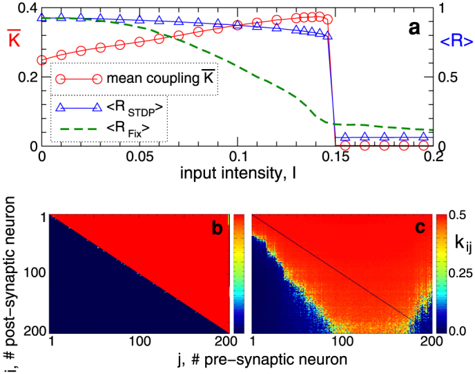
(a), Mean (ensemble-averaged) synaptic weight (scale on the left vertical axis) and the time-averaged order parameters 〈R_STDP〉 and 〈R_Fix〉 (scale on the right vertical axis) for the ensemble with and without STDP, respectively, versus input intensity I. For the network without STDP, the coupling matrix is fixed K_Fix (see Methods). (b), (c), Coupling matrices established in the HH ensemble due to STDP for the input intensity I = 0 in (b) and I = 0.14 in (c), where the synaptic weights k_ij are encoded in color. The elements of the initial coupling matrix K(0) = {k_ij(0)} are Gaussian distributed around the mean value with standard deviation 0.02. For illustration, the neurons are sorted with respect to increasing natural spiking frequency such that f_i ≤ f_j for i < j.

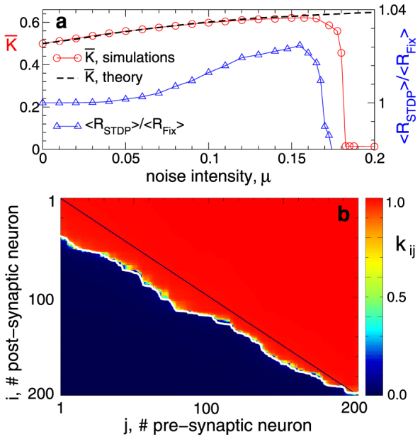
The mechanism behind the reported phenomenon is based on the noise-induced dynamics of the spike time differences Δt_ij used for the update of the synaptic weights [Supplementary Section S1B]. If the distribution density ρ_ij(Δt) of Δt_ij is known, the average update rate of the synaptic weights can be calculated by the integral

where W describes the update rule in one spike event (7). One therefore has to describe the form of ρ_ij in order to predict the dynamics of the coupling weights k_ij: They will be potentiated if and depressed if . For instance, for a uniform distribution ρ_ij = 1/2ε of Δt_ij ∈ [−ε, ε], and changes its sign from positive to negative as ε increases over 5 ms for the considered parameters. Therefore, if Δt_ij are broadly distributed, e.g., for desynchronized neurons at a weak initial coupling, the synaptic weights will be depressed and a weakly coupled regime will be realized. On the other hand, a synchronized firing for a strong initial coupling will lead to narrowly distributed Δt_ij and further stabilization of a strongly coupled regime [Fig. 1b], see also Supplementary Section S1A. Notice that the considered STDP will lead to a potentiation of synaptic weights if the neurons fire at a high rate¹⁷,²⁴. In this case, the relative spike times will be narrowly distributed even if the neurons are not synchronized. In our case the mean firing rate does not significantly change when the parameters of interest vary [Supplementary Fig. S3].

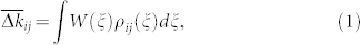
We consider the behavior of ρ_ij in more detail for the phase oscillators (8) with STDP, where we observe the same constructive effect of the independent noise: As the noise intensity increases, so does the mean coupling strength until it reaches its maximal value at the optimal noise intensity μ = μ_opt [Fig. 2a]. As for the HH ensemble, the noise induces the emergence of bidirectional couplings among oscillators [Fig. 2b], and STDP counteracts the suppression of synchronization by the noise [Fig. 2a]. Although the latter effect for the phase ensemble is somewhat less pronounced (regarding 〈R_STDP〉/〈R_Fix〉) than for the HH neurons, we still observe the self-organized resistance to noise for the phase oscillators mediated by STDP, where 〈R_STDP〉 > 〈R_Fix〉.

Figure 2. Constructive effect of independent noise on the coupling of the phase ensemble with STDP.

(a), Mean coupling weight and ratio 〈R_STDP〉/〈R_Fix〉 (scale on the right vertical axis) between the time-averaged order parameters for the ensemble with and without STDP, respectively, versus noise strength μ. In the latter case the coupling matrix is fixed K_Fix (see Methods). (b), Coupling matrix K_STDP established in the phase ensemble due to STDP for the noise intensity μ = 0.1. The dashed black curve in (a) approximates the mean coupling weight , and the white curve in (b) bounds the region of potentiated coupling weights, both as predicted by the theory (see text for details). The oscillators are sorted with respect to increasing natural frequencies ω_i which are uniformly and randomly distributed in the interval [0.9, 1.1].

We found that the emergence of positive couplings below the diagonal in the coupling matrix [Fig. 2b] of the phase ensemble can be explained by evaluating the impact of the noise on the phase differences for fixed coupling matrix K_Fix, and we consider such a system below.

In the strongly coupled regime without noise the oscillators are phase locked and the phase differences are constant. The following recurrent formula gives the constant phase shifts of the locked phases ψ_i = ωt + ϕ_i (see Supplementary Section S2A):

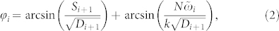where , , , and . Letting ϕ_N = 0, without loss of generality, we find the constant phase differences Δψ_ij = ϕ_j − ϕ_i. For weak to moderate noise the phase differences fluctuate around the above mean values and get broadly distributed, see Fig. 3a, Supplementary Section S2B, and Refs. ^{25, 26}. Since the phase differences obey a circular statistics we approximate them in the noisy case by the von Mises distribution²⁷

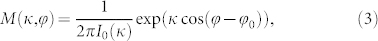where I₀(κ) is the modified Bessel function of first kind and zero order, κ is the concentration parameter, and ϕ₀ is the mean value. The parameter κ(Δψ_ij) can be determined and demonstrates a power-law dependence on the noise strength μ [Fig. 3b]

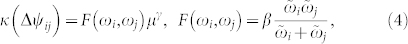where the exponent γ ≈ −2 seems to be independent of the natural frequencies ω_i and ω_j [Fig. 3b and Supplementary Section S2B]. We therefore represent the dependence of parameter κ(Δψ_ij) on the natural frequencies as a function F(ω_i, ω_j) in equation (4). Detailed numerical calculations reveal that the contour lines F(ω_i, ω_j) = F_const of the function F align along the hyperbolas 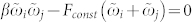for some constant β, where β ≈ −9.52 for the considered fixed other parameters of the system, see Supplementary Section S2C.

Figure 3. Impact of the noise-induced dynamics of the phase differences on coupling weights of the phase ensemble.

(a), Noise-induced distribution densities ρ_ij of the phase differences Δψ_ij(μ) between the post-synaptic oscillator i = 100 and pre-synaptic oscillators j indicated in the plot. The hatched histograms illustrate the results of numerical simulations for noise intensity μ = 0.1, the enveloping dashed black curves depict the von Mises distribution (3) for fitted κ, and the vertical lines are delta-peak distributions for the noise-free case according to equation (2). (b), Log-log plot of parameter κ(Δψ_ij) of the fitted von Mises distribution (3) versus μ for oscillator pairs (i, j) indicated in the plot. The dashed black lines have the slope −2. (c), The average update rate of the coupling weights. The black dashed curves depict the theoretical approximation calculated according to equations (1)–(4) with γ = −2 and β = −9.52, while the symbols represent the results of numerical simulations. Vertical dashed lines indicate the index j where the predicted crosses zero. In plots (a)–(c) coupling matrix is fixed to K_Fix (see Methods). (d), Time-averaged coupling weights 〈k_100,j〉 established in the phase ensemble with STDP for noise intensities as in plot (c). Natural frequencies ω_i = 0.9 + 0.2(i − 1)/(N − 1), i = 1, 2, …, N, N = 200.

With the use of equation (4) one can predict the noise-induced emergence of positive coupling k_ij from slow oscillators to fast ones, (for indices j < i in Fig. 2b). For this, the STDP function (7) can be integrated with respect to the distribution density ρ(Δψ_ij) of the form (3) according to equation (1) for the mean phase differences (2) and parameter κ from equation (4) with the obtained parameters γ and β. The results of such an approximation are illustrated in Figs. 3c, d, where the range of potentiated coupling weights increases as predicted by [Fig. 3c] which is in good accordance with the numerical simulations for weak to moderate noise [Fig. 3d]. Moreover, the above equations can effectively be used to approximate the mean coupling [Fig. 2a] and the shape of the coupling matrix with irregular border between potentiated and depressed coupling weights [Fig. 2b] for randomly distributed natural frequencies.

Strong noise destroys the synchronization in the HH and phase ensembles, which, in turn, leads to a depression of the coupling among oscillators by STDP, and the mean coupling weight nearly vanishes [Figs. 1a and 2a]. We found that the onset of decoupling originates from the fast oscillators (large index j in Figs. 1c and 2b) and propagates to the interior of the coupling matrix as time evolves, see Supplementary Videos 1 and 2 for the animated time courses of the coupling matrices of the HH and phase ensembles, respectively. The indication of such a decoupling mechanism can be obtained from the population without STDP and fixed coupling matrix K_Fix (see Methods). Already for μ = μ_opt = 0.1625 the coupling weights k_ij from the fastest oscillators are predicted to be depressed by STDP as, for example, for i = 100 and j = 200, where [Fig. 3c]. This indicates that the suppression of the coupling for large noise will start from the fastest oscillators.

For the same parameters of the STDP function (7) the self-organized resistance against noise is significantly enhanced for another, multiplicative (state-dependent) update rule, where the coupling weights are changed relative to their current values k_ij → k_ij + (k_M − k_ij)|δW(Δψ_ij)|, where k_M = k_max or k_M = k_min depending on whether the coupling update δW(Δψ_ij) is positive (potentiation) or negative (depression), respectively²⁸. Even for strong independent noise the oscillators with such a coupling update remain strongly coupled and synchronized [Fig. 4a]. The dynamics of the coupling matrix is, however, different for this update rule [Fig. 4b]. As the noise strength increases, the coupling weights k_ij converge from a strictly bimodal distribution for the noise-free case via a nearly uniform distribution to a well-pronounced uni-modal distribution of approximately globally coupled oscillators for strong noise. The latter distribution is in accordance with the results of Ref. 28. Interestingly, the oscillators are coupled with about the same mean coupling in the noise-free case (μ = 0) and for strong noise (μ = 0.5) [Fig. 4a]. In the latter case, however, the population with STDP is much more resistant to noise than the population without STDP, while both have the same mean coupling. This also indicates that the global coupling with narrowly distributed coupling weights [Fig. 4b] is more favorable if robustness of the synchronized dynamics against noise is required. These findings also contribute to the problem of the optimal coupling topology for easily synchronizable networks and their resistance to noise²⁹.

Figure 4. Constructive effect of independent noise on the coupling of the phase ensemble with multiplicative (state-dependent) coupling update.

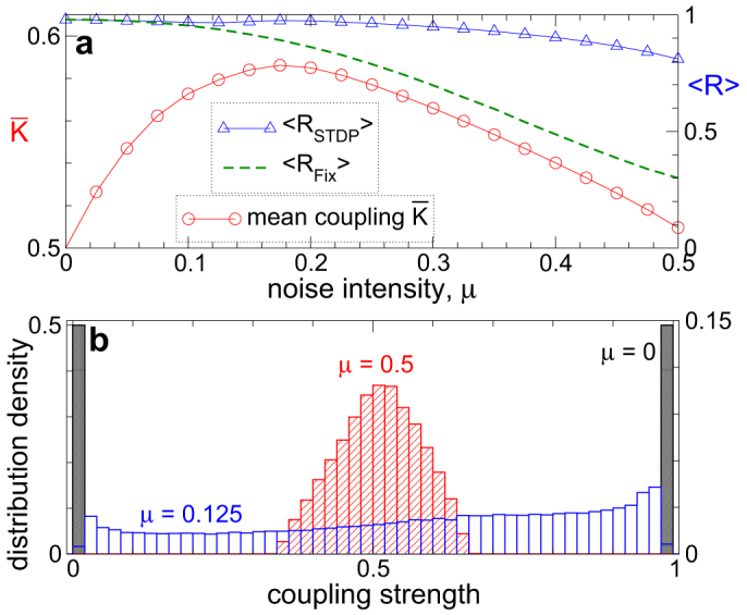
(a), Mean synaptic weight (scale on the left vertical axis) and time-averaged order parameters 〈R_STDP〉 and 〈R_Fix〉 (scale on the right vertical axis) for the ensemble with STDP and without STDP (for fixed coupling matrix K_Fix, see Methods), respectively, versus noise strength μ. (b), Normalized histograms of the distribution density of the coupling weights k_ij for the noise intensities μ = 0 (no input, scale on the left vertical axis), μ = 0.125 and μ = 0.5 (scale on the right vertical axis) as indicated in the plot.

Discussion

We demonstrated the constructive impact of independent noise on ensembles of oscillatory HH neurons and phase oscillators with asymmetric STDP and for two different protocols of the coupling update based on the difference of either the spike timing or the phases. In the latter case the coupling update is separated from possible changes of the frequencies, which means that the reported phenomenon is in fact based on the phase dynamics. This mechanism is different as compared to stochastic or coherence resonances³⁰,³¹,³², where the interplay between noise-induced and internal or external times scales is important. Indeed, the noisy input does not significantly change the frequency of the synchronized neurons and only influences the distribution of the phase differences by broadening it [Fig. 3]. This results in a potentiation of the synaptic weights that were depressed in the noise-free case.

For the phase model we provided a theoretical approximation of the structure of the coupling matrix, which is in good agreement with the results of the numerical simulations. For the HH ensemble we also verified the reported phenomenon for a random synaptic inhibitory input and somatic Gaussian noise as well as for different spike pairing for STDP [Supplementary Section S1C]. Furthermore, we verified the phenomenon for different parameter sets for the plasticity function and found that the noise-induced increase of synaptic weights gets more pronounced if the STDP function is shaped for a stronger potentiation rather than for depression. In this study we however considered a non-trivial case, where strongly coupled synchronized and weakly coupled desynchronized states stably coexist if the communication delay among neurons is small, and synchronization is associated with large coupling³³,³⁴. In general, the noise-induced increase of the mean coupling can be expected for an asymmetric STDP rule if the neurons can be in-phase locked with narrowly distributed spike time differences, and a uni-directional coupling topology like in Fig. 1b is established in the noise-free case.

The resonance-like behavior of the mean coupling versus noise intensity has been observed for both multiplicative and additive coupling update rules, where the coupling update either depends or not, respectively, on the current value of the synaptic weight and leads to “soft” or “hard” bounds, accordingly²³,²⁸. The distribution of synaptic weights however is always bimodal for hard bounds [Figs. 1 and 2], whereas it undergoes a gradual transformation from a bimodal to a uniform distribution and then to a relatively narrow unimodal distribution as noise strength increases for soft bounds [Fig. 4], see also Refs. ^{23, 28}. These findings point to the robustness and generality of the reported phenomenon.

Our results suggest a possible homeostatic mechanism of how the brain may counteract external perturbations and noise in order to preserve the existing level of neural synchrony and bridge the transition from information coding by precise spike times to variable and imperfect spike timing. Noise leads to the development of bidirectional coupling among neurons observed in experiments³⁵. Furthermore, our results show that independent noise can by no means be considered as an effective method for desynchronization of oscillatory neural networks with STDP. Also from the clinical standpoint our results may be important. In fact, they may contribute to a deeper understanding of why maskers and noisers show limited efficacy in counteracting tinnitus³⁶, the latter being associated with abnormal neural synchrony⁴,²⁰.

Methods

Hodgkin-huxley (HH) ensemble

The considered system of N synaptically interacting spiking HH neurons³⁷,³⁸ reads

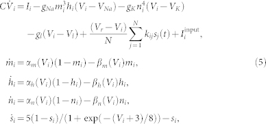where the variable V_i, i = 1, …, N, models the membrane potential of neuron i, and α_m(V) = (0.1 V + 4)/[1 − exp(−0.1 V − 4)], β_m(V) = 4 exp((−V − 65)/18), α_h(V) = 0.07 exp((−V − 65)/20), β_h(V) = 1/[1 + exp(−0.1 V − 3.5)], α_n(V) = (0.01 V + 0.55)/[1 − exp(−0.1 V − 5.5)], and β_n(V) = 0.125 exp((−V − 65)/80). Parameters C = 1 μF/cm², V_Na = 50 mV, V_K = −77 mV, V_l = −54.4 mV, g_Na = 120 mS/cm², g_K = 36 mS/cm², g_l = 0.3 mS/cm².

The neurons are excitatorily coupled (with reversal potential V_r = 20 mV) via the post-synaptic potentials (PSP) s_i with synaptic weights k_ij modeling the strength of the coupling from the pre-synaptic neuron j to the post-synaptic neuron i. We consider the case without self-coupling k_ii = 0. The constant currents I_i are randomly and uniformly distributed in the interval [10.5; 11.5] μA/cm². For such parameters I_i the spiking frequencies f_i (number of spikes per second) of the uncoupled neurons (k_ij = 0) without an external input () get distributed around the mean value 70.7 Hz with standard deviation 0.62 Hz. For numerical integration of model (5) with synaptic input we used a Runge-Kutta method of order 5(4) with adaptive step size³⁹.

Independent random input

The excitatory synaptic input current reads

The α-train in equation (6) models the PSPs received by neuron i at times τ_i,k with inter-spike intervals Δτ_i,k = τ_i,k+1 − τ_i,k ≥ 0 independently drawn from a Gaussian distribution with mean 〈Δτ_i,k〉 = 14 ms and standard deviation 4 ms, and α = 24/〈Δτ_i,k〉. The mean inter-spike interval of such an input approximately equals the mean period of the coupling- and input-free neurons (5), and each neuron receives an independent random synaptic input of intensity I, which does not significantly perturb its natural spiking frequency, see Supplementary Fig. S3.

Spike timing-dependent plasticity (STDP)

The neural ensemble (5) is equipped with STDP¹⁴,¹⁵,¹⁶,¹⁷, where the synaptic weights k_ij = k_ij(t) are updated in a point process-like manner as according to the following STDP function when the post-synaptic neuron i or the pre-synaptic neuron j fires:

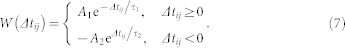Δt_ij = t_i − t_j is the time difference between the nearest spike onsets of the neurons i and j. The spike onsets are detected by the upward zero crossing by the membrane potential following an inter-spike hyperpolarization. If the time difference Δt_ij is negative (the spike of the post-synaptic neuron advances that of the pre-synaptic neuron), the corresponding synaptic weight is depressed, otherwise, it is potentiated. Since STDP acts on a slower time scale than the underlying neural activity, we consider a slow changing rate of the synaptic weights δ = 0.001, see also Refs. ^{14, 17}. It also prevents from spuriously moving away from a branch of attractors known as R-tipping⁴⁰. The synaptic weights k_ij are confined to the interval [k_min, k_max] = [0, 0.5] by setting k_ij to k_min as soon as k_ij tends to be depressed below k_min via STDP or, respectively, to k_max if k_ij is potentiated beyond this value.

We consider parameters A₁ = 1, A₂ = 0.5, τ₁ = 1.8, and τ₂ = 6 such that, if the input is absent (), STDP can lead to a multistability of a weakly coupled asynchronous state and a strongly coupled synchronized state, see Supplementary Section S1A and Refs. ^{18, 41}. Depending on the initial coupling, the mean coupling saturates at in the weakly coupled regime and at in the strongly coupled regime, and the synchronization order parameter¹¹ is on average 〈R〉 ≈ 0.28 and 〈R〉 ≈ 0.92, respectively. Here, ψ_j(t) = 2π(t − t_j,m)/(t_j,m+1 − t_j,m), t_j,m ≤ t < t_i,m+1, m = 0, 1, 2, …, approximates the phase of neuron j, and t_j,m are the times of its spike onsets. For , the mean coupling [Fig. 1a], and the established uni-directional hierarchical coupling topology [Fig. 1b] results from the asymmetry of the STDP rule (7) and a phase locking of the neurons to each other, see Supplementary Section S1A and Refs. ^{42, 43}.

Phase oscillators with STDP

We also consider the Kuramoto phase ensemble¹¹ with independent noise

where the coupling weights k_ij obey the STDP rule (7) with parameters A₁ = 1, A₂ = 0.5, τ₁ = 0.45, τ₂ = 1.5, and δ = 0.005, and are confined to the interval k_ij ∈ [k_min, k_max] with k_min = 0 and k_max = 1. The update (7) of the coupling coefficients is based on the phase difference W = W(Δψ_ij), Δψ_ij = ψ_j − ψ_i, between the pre- and postsynaptic oscillators j and i, respectively, and undertaken when their phases cross zero (mod 2π), which is declared as a spike onset if the phase visited an “inter-spike” value π (mod 2π) just before. The phase-based STDP was chosen in order to avoid any influence of the frequency dynamics and to show that the discussed effects are based on the noise-induced dynamics of the phase differences. The phase oscillators (8) are perturbed by a normally distributed independent noise ξ_i with 〈ξ_i〉 = 0 and 〈ξ_i(t), ξ_j(t′)〉 = δ(i − j)δ(t − t′), and intensity μ. The natural frequencies ω_i are uniformly and randomly distributed in the interval [0.9, 1.1]. In calculations for fitting the noise-induced distribution of the phase differences we also used a regular distribution ω_i = 0.9 + 0.2(i − 1)/(N − 1). For numerical integration of model (8) with noise input we used the Heun method⁴⁴ with step size 0.01.

As for the HH neural ensemble, the noise-free (μ = 0) phase ensemble (8) with the phase-based STDP (7) demonstrates a multistability of a weakly coupled asynchronous regime (with and 〈R〉 ≈ 0.4) and a strongly coupled synchronized regime (with and 〈R〉 ≈ 0.98). In the latter regime a uni-directional hierarchical coupling from fast to slow oscillators is established, similarly to the HH neural population, see Fig. 1b.

Fixed coupling

To compare the effect of the noise for the HH and phase ensembles with STDP to those without STDP, in the latter case the coupling matrix was fixed to K_Fix = {k_ij}, where k_ij = k = k_max/2 for i < j, and k_ij = 0 otherwise (the oscillators are sorted with respect to increasing natural frequency), as for the strongly coupled regimes established without noise.

Author Contributions

O.V.P. designed the specific mathematical analysis, performed numerical simulations and theoretical approximations, and prepared the manuscript. O.V.P., S.Y. and P.A.T. discussed the results, drew conclusions and edited the manuscript. P.A.T. supervised the study.

Supplementary Material

Supplementary Information

Supplementary Video 1

Supplementary Information

Supplementary Video 2

Supplementary Information

Supplementary Info

References

- Singer W. Synchronization of cortical activity and its putative role in information processing and learning. Annu. Rev. Physiol. 55, 349–374 (1993). [DOI] [PubMed] [Google Scholar]
- Engel A. K., Fries P. & Singer W. Dynamic predictions: Oscillations and synchrony in top-down processing. Nature Rev. Neurosci. 2, 704–716 (2001). [DOI] [PubMed] [Google Scholar]
- Hammond C., Bergman H. & Brown P. Pathological synchronization in parkinson's disease: networks, models and treatments. Trends Neurosci. 30, 357–364 (2007). [DOI] [PubMed] [Google Scholar]
- Roberts L. E. et al. Ringing ears: The neuroscience of tinnitus. J. Neurosci. 30, 14972–14979 (2010). [DOI] [PMC free article] [PubMed] [Google Scholar]
- Tass P. A. & Popovych O. V. Unlearning tinnitus-related cerebral synchrony with acoustic coordinated reset stimulation: theoretical concept and modelling. Biol. Cybern. 106, 27–36 (2012). [DOI] [PubMed] [Google Scholar]
- Tass P. A. Phase resetting in medicine and biology: stochastic modelling and data analysis (Springer, Berlin, 1999). [Google Scholar]
- Tass P. A. A model of desynchronizing deep brain stimulation with a demand-controlled coordinated reset of neural subpopulations. Biol. Cybern. 89, 81–88 (2003). [DOI] [PubMed] [Google Scholar]
- Rosenblum M. G. & Pikovsky A. S. Controlling synchronization in an ensemble of globally coupled oscillators. Phys. Rev. Lett. 92, 114102 (2004). [DOI] [PubMed] [Google Scholar]
- Popovych O. V., Hauptmann C. & Tass P. A. Effective desynchronization by nonlinear delayed feedback. Phys. Rev. Lett. 94, 164102 (2005). [DOI] [PubMed] [Google Scholar]
- Kiss I. Z., Rusin C. G., Kori H. & Hudson J. L. Engineering complex dynamical structures: Sequential patterns and desynchronization. Science 316, 1886–1889 (2007). [DOI] [PubMed] [Google Scholar]
- Kuramoto Y. Chemical oscillations, waves, and turbulence (Springer, Berlin, 1984). [Google Scholar]
- Sakaguchi H. Cooperative phenomena in coupled oscillator systems under external fields. Prog. Theor. Phys. 79, 39–46 (1988). [Google Scholar]
- Strogatz S. H. & Mirollo R. E. Stability of incoherence in a population of coupled oscillators. J. Stat. Phys. 63, 613–635 (1991). [Google Scholar]
- Gerstner W., Kempter R., van Hemmen J. L. & Wagner H. A neuronal learning rule for sub-millisecond temporal coding. Nature 383, 76–78 (1996). [DOI] [PubMed] [Google Scholar]
- Markram H., Lübke J., Frotscher M. & Sakmann B. Regulation of synaptic efficacy by coincidence of postsynaptic APs and EPSPs. Science 275, 213–215 (1997). [DOI] [PubMed] [Google Scholar]
- Bi G.-Q. & Poo M.-M. Synaptic modifications in cultured hippocampal neurons: dependence on spike timing, synaptic strength, and postsynaptic cell type. J. Neurosci. 18, 10464–10472 (1998). [DOI] [PMC free article] [PubMed] [Google Scholar]
- Clopath C., Busing L., Vasilaki E. & Gerstner W. Connectivity reflects coding: a model of voltage-based stdp with homeostasis. Nature Neurosci. 13, 344–352 (2010). [DOI] [PubMed] [Google Scholar]
- Tass P. A. & Majtanik M. Long-term anti-kindling effects of desynchronizing brain stimulation: a theoretical study. Biol. Cybern. 94, 58–66 (2006). [DOI] [PubMed] [Google Scholar]
- Tass P. A. & Hauptmann C. Therapeutic modulation of synaptic connectivity with desynchronizing brain stimulation. Int. J. Psychophysiol. 64, 53–61 (2007). [DOI] [PubMed] [Google Scholar]
- Tass P., Adamchic I., Freund H.-J., von Stackelberg T. & Hauptmann C. Counteracting tinnitus by acoustic coordinated reset neuromodulation. Rest. Neurol. Neurosci. 30, 367–374 (2012). [DOI] [PubMed] [Google Scholar]
- Tass P. A. et al. Coordinated reset has sustained aftereffects in parkinsonian monkeys. Ann. Neurol. 72, 816–820 (2012). [DOI] [PubMed] [Google Scholar]
- Silchenko A. N., Adamchic I., Hauptmann C. & Tass P. A. Impact of acoustic coordinated reset neuromodulation on effective connectivity in a neural network of phantom sound. Neuroimage 77, 133–147 (2013). [DOI] [PubMed] [Google Scholar]
- Song S., Miller K. & Abbott L. Competitive hebbian learning through spike-timing-dependent synaptic plasticity. Nat. Neurosci. 3, 919–926 (2000). [DOI] [PubMed] [Google Scholar]
- Fushiki T. & Aihara K. A phenomenon like stochastic resonance in the process of spike-timing dependent synaptic plasticity. IEICE Trans. Fundamentals E85A, 2377–2380 (2002). [Google Scholar]
- Nakao H., Arai K. & Kawamura Y. Noise-induced synchronization and clustering in ensembles of uncoupled limit-cycle oscillators. Phys. Rev. Lett. 98, 184101 (2007). [DOI] [PubMed] [Google Scholar]
- Ly C. & Ermentrout G. B. Synchronization dynamics of two coupled neural oscillators receiving shared and unshared noisy stimuli. J. Comput. Neurosci. 26, 425–443 (2009). [DOI] [PubMed] [Google Scholar]
- Mardia K. & Jupp P. Directional Statistics (Wiley, Chichester, 2009). [Google Scholar]
- Rubin J., Lee D. D. & Sompolinsky H. Equilibrium properties of temporally asymmetric hebbian plasticity. Phys. Rev. Lett. 86, 364–367 (2001). [DOI] [PubMed] [Google Scholar]
- Yanagita T. & Mikhailov A. S. Design of oscillator networks with enhanced synchronization tolerance against noise. Phys. Rev. E 85, 056206 (2012). [DOI] [PubMed] [Google Scholar]
- Pikovsky A. S. & Kurths J. Coherence resonance in a noise-driven excitable system. Phys. Rev. Lett. 78, 775–778 (1997). [Google Scholar]
- Neiman A., Saparin P. I. & Stone L. Coherence resonance at noisy precursors of bifurcations in nonlinear dynamical systems. Phys. Rev. E 56, 270–273 (1997). [Google Scholar]
- Moss F., Ward L. M. & Sannita W. G. Stochastic resonance and sensory information processing: a tutorial and review of application. Clin. Neurophysiol. 115, 267–281 (2004). [DOI] [PubMed] [Google Scholar]
- Lubenov E. V. & Siapas A. G. Decoupling through synchrony in neuronal circuits with propagation delays. Neuron 58, 118–131 (2008). [DOI] [PubMed] [Google Scholar]
- Mikkelsen K., Imparato A. & Torcini A. Emergence of slow collective oscillations in neural networks with spike-timing dependent plasticity. Phys. Rev. Lett. 110, 208101 (2013). [DOI] [PubMed] [Google Scholar]
- Song S., Sjöström P., Reigl M., Nelson S. & Chklovskii D. Highly nonrandom features of synaptic connectivity in local cortical circuits. PLoS Biol. 3, 507–519 (2005). [DOI] [PMC free article] [PubMed] [Google Scholar]
- Hobson J., Chisholm E. & Refaie E. A. Sound therapy (masking) in the management of tinnitus in adults. Cochrane Database of Systematic Reviews 11, CD006371 (2012). [DOI] [PMC free article] [PubMed] [Google Scholar]
- Hodgkin A. & Huxley A. F. A quantitative description of membrane current and application to conduction and excitation. J. Physiol. 117, 500–544 (1952). [DOI] [PMC free article] [PubMed] [Google Scholar]
- Hansel D., Mato G. & Meunier C. Phase dynamics of weakly coupled Hodgkin-Huxley neurons. Europhys. Lett. 23, 367–372 (1993). [Google Scholar]
- Hairer E., Nørsett S. & Wanner G. Solving ordinary differential equations I: nonstiff problems (Springer, Berlin, 1993). [Google Scholar]
- Ashwin P., Wieczorek S., Vitolo R. & Cox P. Tipping points in open systems: bifurcation, noise-induced and rate-dependent examples in the climate system. Philos. Trans. R. Soc. A 370, 1166–1184 (2012). [DOI] [PubMed] [Google Scholar]
- Popovych O. V. & Tass P. A. Desynchronizing electrical and sensory coordinated reset neuromodulation. Front. Hum. Neurosci. 6, 58 (2012). [DOI] [PMC free article] [PubMed] [Google Scholar]
- Masuda N. & Kori H. Formation of feedforward networks and frequency synchrony by spike-timing-dependent plasticity. J. Comput. Neurosci. 22, 327–345 (2007). [DOI] [PubMed] [Google Scholar]
- Bayati M. & Valizadeh A. Effect of synaptic plasticity on the structure and dynamics of disordered networks of coupled neurons. Phys. Rev. E 86, 011925 (2012). [DOI] [PubMed] [Google Scholar]
- Greiner A., Strittmatter W. & Honerkamp J. Numerical integration of stochastic differential equations. J. Stat. Phys. 51, 95–108 (1988). [Google Scholar]
Associated Data
This section collects any data citations, data availability statements, or supplementary materials included in this article.
Supplementary Materials