A Study of the Morpho-Semantic Relationship in Medline

Abstract

Morphological analysis as applied to English has generally involved the study of rules for inflections and derivations. Recent work has attempted to derive such rules from automatic analysis of corpora. Here we study similar issues, but in the context of the biological literature. We introduce a new approach which allows us to assign probabilities of the semantic relatedness of pairs of tokens that occur in text in consequence of their relatedness as character strings. Our analysis is based on over 84 million sentences from the MEDLINE database, over 2.3 million token types that occur in MEDLINE, and enables us to identify over 36 million token type pairs which have assigned probabilities of semantic relatedness of at least 0.7 based on their similarity as strings. The quality of these predictions is tested by two different manual evaluations and found to be good.

Introduction

Morphological analysis is an important element in natural language processing. Jurafsky and Martin [1] define morphology as the study of the way words are built up from smaller meaning bearing units, called morphemes. Robust tools for morphological analysis enable one to predict the root of a word and its syntactic class or part of speech in a sentence. Stemming algorithms [2] use basic knowledge of grammar to eliminate recognized suffixes, leaving a putative root word. A good deal of work has also been done toward the automatic acquisition of rules, morphemes, and analyses of words from large corpora [3-12]. While this work is important it is mostly concerned with inflectional and derivational rules that can be derived from the study of texts in a language. While our interest is related to this work, we are concerned with the multitude of tokens that appear in English texts on the subject of biology. We believe it is clear to anyone who has examined the literature on biology that there are many tokens that appear in textual material that are related to each other, but not in any standard way or by any simple rules that have general applicability even in biology. It is our goal here to achieve some understanding of when two tokens can be said to be semantically related based on their similarity as strings of characters.

Thus for us morphological relationship will be a bit more general in that we wish to infer the relatedness of two strings based on the fact that they have a certain substring of characters on which they match. But we do not require knowledge of exactly on what part of the matching substring their semantic relationship depends. In other words we do not insist on the identification of the smaller meaning bearing units or morphemes. Key to our approach is the ability to measure the contextual similarity between two token types as well as their similarity as strings. Neither kind of measurement is unique to our application. Contextual similarity has been studied and applied in morphology [8, 11, 13, 14] and more generally [15]. String similarity has also received much attention [16-23]. However, the way we use these two measurements is, to our knowledge, new. Our approach is based on a simple postulate: If two token types are similar as strings, but they are not semantically related because of their similarity, then their contextual similarity is no greater then would be expected for two randomly chosen token types. Based on this observation we carry out an analysis which allows us to assign a probability of relatedness to pairs of token types. This proves sufficient to generate a large repository of related token type pairs among which are the expected inflectionally and derivationally related pairs and much more besides.

The paper is organized as follows. We begin by defining contextual and lexical similarity. These definitions are then followed by a description of the method by which they are used to estimate the probability of semantic relatedness of two tokens. The lexical similarity is initially based on IDF weights of the substring features used. This was initially chosen because IDF weighting is a way to account for the information conveyed by a string based on its frequency in a dataset and is quite successfully used in information retrieval applications [24, 25]. We find by experiment that weighting all features with the value 1.0 is more effective than IDF weights and we introduce a procedure for learning these weights which provides even greater sensitivity. These results are followed by an evaluation of the accuracy of the predicted probabilities and we show by direct human judgments as well as by an application to improve the Porter stemmer that the predictions are indeed close to what humans would predict. Given the learned weights and the resulting probability estimates we show how to summarize all the data to produce probability estimates that two tokens are semantically related based on their lexical similarity alone. The fact that the resulting probability estimates are linearly related to the lexical similarity score, we believe, provides some support for the machine learning approach used. The paper ends with a discussion and conclusion section. A preliminary and abridged version of this work appeared in the past [26], but the current work gives a thorough analysis of the machine learning approach used and a formal evaluation of the probabilities predicted confirming their accuracy.

Data

A March 2007 copy of MEDLINE was used for this study. In the first step all the MEDLINE documents were broken into sentences using the MedPost [27] sentence segmenting function available on SourceForge under the title “medpost” . This produced a set of 84,475,092 sentences. The sentences were then tokenized by breaking at all non-alphanumeric characters including spaces, tabs, and punctuation. The resulting tokens that contained at least one alphabetic character were retained for analysis. This resulted in 2,341,917 token types and these are the subject of our study.

Measuring Contextual Similarity

In considering the context of a token in a MEDLINE record we do not consider all the text of the record. In those cases when there are multiple sentences in the record the text that does not occur in the same sentence as the token may be too distant to have any direct bearing on the interpretation of the token and will in such cases add noise to our considerations. Thus we break MEDLINE records into sentences and consider the context of a token to be the additional tokens of the sentence in which it occurs. Likewise the context of a token type consists of all the additional token types that occur in all the sentences in which it occurs. While there is an advantage in the specificity that comes from considering context at the sentence level, this approach also gives rise to a problem. It is not uncommon for two terms to be related semantically, but to never occur in the same sentence. This will happen, for example, if one term is a miss-spelling of the other or if the two terms are alternate names for the same object. Because of this we must estimate the context of each term without regard to the occurrence of the other term. Then the two estimates can be compared to compute a similarity of context. We accomplish this using formulas of probability theory applied to our setting.

Let T denote the set of 2,341,917 token types we consider and let t₁ and t₂ be two token types we wish to compare. Then we define

$$p_c(t_1)={\sum }_{i\in T}p(t_1|i)p(i)\text{and}{p}_c(t_2)={\sum }_{i\in T}p(t_2|i)p(i).$$ (1)

Here we refer to p_c(t₁) and p_c(t₂) as contextual probabilities for t₁ and t₂, respectively. The expressions on the right sides in (1) are given the standard interpretations. Thus p(i) is the fraction of tokens in MEDLINE that are equal to i and p(t₁ | i) is the fraction of sentences in MEDLINE that contain i that also contain t₁. We make a similar computation for the pair of token types

$$p_c(t_1\wedge t_2)={\sum }_{i\in T}p(t_1\wedge t_2|i)p(i)={\sum }_{i\in T}p(t_1|i)p(t_2|i)p(i).$$ (2)

Here we have made use of an additional assumption, that given i, t₁ and t₂ are independent in their probability of occurrence. While independence is not true, this seems to be just the right assumption for our purposes. It allows our estimate of p_c (t₁ ∧ t₂) to be nonzero even though t₁ and t₂ may never occur together in a sentence. In other words it allows our estimate to reflect what context would imply if there were no rule that says the same intended word will almost never occur twice in a single sentence, etc. Our contextual similarity is then the mutual information based on contextual probabilities

$$\mathit{\text{conSim}}=(t_1,t_2)=log\left(\frac{p_c(t_1\wedge t_2)}{p_c(t_1)p_c(t_2)}\right)$$ (3)

There is one minor practical difficulty with this definition. There are many cases where p_c(t₁ ∧ t₂) is zero. In any such case we define conSim(t₁,t₂) to be -1000.

Measuring Lexical Similarity

Here we treat the two token types, t₁ and t₂ of the previous section, as two ASCII strings and ask how similar they are as strings. String similarity has been studied from a number of viewpoints [16-23]. We avoided approaches based on edit distance or other measures designed for spell checking because our problem requires the recognition of relationships more distant than simple miss-spellings. Our method is based on character ngrams as features to represent any string [19, 20, 22, 23]. If t = “abcdefgh” represents a token type, then we define F(t) to be the feature set associated with t and we take F(t) to be composed of i) all the contiguous three character substrings “abc”, “bcd”, “cde”, “def”, “efg”, and “fgh”; ii) the specially marked first trigram “abc!”; and iii) the specially marked first letter “a #”. This is the form of F(t) for any t at least three characters long. If t consists of only two characters, say “ab”, we take i) “ab”; ii) “ab!”; and iii) is unchanged. If t consists of only a single character “a”, we likewise take i) “a”; ii) “a!”; and iii) is again unchanged. Here ii) and iii) are included to allow the emphasis of the beginning of strings as more important for their recognition than the remainder. We emphasize that F(t) is a set of features, not a “bag-of-words”, and any duplication of features is ignored. While this is a simplification, it does have the minor drawback that different strings, e.g., “aaab” and “aaaaab”, are represented by the same set of features.

Given that each string is represented by a set of features, it remains to define how we compute the similarity between two such representations. Our basic assumption here is that the probability p(t₂ | t₁), that the semantic implications of t₁ are also represented at some level in t₂, should be represented by the fraction of the features representing t₁ that also appear in t₂. Of course there is no reason that all features should be considered of equal value. Let F denote the set of all features coming from all 2.34 million strings we are considering. We will make the assumption that there exists a set of weights w(f) defined over all of f ∈ F and representing their semantic importance. Then we have

$$p(t_2|t_1)={\sum }_{f\in {F(t}_1)\cap {F(t}_2)}w(f)/{\sum }_{f\in F(t_1)}w(f).$$ (4)

Based on (4) we define the lexical similarity of two token types as

$$\mathit{\text{lexSim}}(t_1,t_2)=(p(t_2|t_1)+p(t_1|t_2))/2$$ (5)

In our initial application of lexSim we take as weights the so-called inverse document frequency weights that are commonly used in information retrieval [28]. If N = 2,341,917 , the number of token types, and for any feature f, n_f represents the number of token types with the feature f, the inverse document frequency weight is

$$w(f)=log\left(\frac{N}{n_f}\right).$$ (6)

This weight is based on the observation that very frequent features tend not to be very important, but importance increases on the average as frequency decreases.

Estimating Semantic Relatedness

The first step is to compute the distribution of conSim(t₁,t₂) over a large random sample of pairs of token types t₁ and t₂. For this purpose we computed conSim(t₁,t₂) over a random sample of 302,515 pairs. This resulted in the value -1000, 180,845 times (60% of values). The remainder of the values, based on nonzero p_c(t₁ ∧ t₂) are distributed as shown in Figure 1.

Figure 1.

Distribution of conSim values for the 40% of randomly selected token type pairs which gave values above -1000, i.e., for which p_c(t₁ ∧ t₂) > 0.

Let τ denote the probability density for conSim(t₁,t₂) over random pairs t₁ and t₂. Let Sem(t₁,t₂) denote the predicate that asserts that t₁ and t₂ are semantically related in the sense that a competent English speaker would judge two tokens to be semantically related (different forms or different spellings of the same word or words referring to closely related concepts). A key point here is that it is unlikely two randomly chosen tokens will be judged semantically related. Then our main assumption which underlies the method is

Postulate. For any nonnegative real number r ≤ 1

$$Q=\left\{\mathit{\text{conSim}}(t_1,t_2)|\mathit{\text{lexSim}}(t_1,t_2)>r\wedge \neg \mathit{\text{Sem}}(t_1,t_2)\right\}$$ (7)

has probability density function equal to τ.

This postulate says that if you have two token types that have some level of similarity as strings (lexSim(t₁,t₂) > r) but which are not semantically related, then lexSim(t₁,t₂) > r is just an accident and it provides no information about conSim(t₁,t₂).

The next step is to consider a pair of real numbers 0 ≤ r₁ < r₂ ≤ 1 and the set

$$S(r_1,r_2)=\left\{(t_1,t_2)|r_1\le \mathit{\text{lexSim}}(t_1,t_2)<r_2\right\}$$ (8)

they define. We will refer to such a set as a lexSim slice. According to our postulate the subset of S(r₁,r₂) which are pairs of tokens without a semantic relationship will produce conSim values obeying the τ density. We compute the conSim values and assume that all of those pairs that produce a conSim value of -1000 represent pairs that are unrelated semantically. As an example, in one of our computations we computed a slice S(0.7,0.725) and found the lexSim value -1000 produced 931,042 times.

In comparing this with the random sample which produced 180,845 values of -1000, we see that

$$\frac{\mathrm{931,042}}{\mathrm{180,845}}=5.148$$ (9)

So we need to multiply the density for the random sample (shown in Figure 1) by 5.148 to represent the part of the slice S(0.7,0.725) that represents pairs not semantically related. This situation is illustrated in Figure 2. Two observations are important here. First, the two curves match almost perfectly along their left edges for conSim values below zero.

Figure 2.

The distribution based on the random sample of pairs represents those pairs in the slice that are not semantically related, while the portion between the two curves represents the number of semantically related pairs.

This suggests that sematically related pairs do not produce conSim scores below about -1 and adds some credibility to our assumption that semantically related pairs do not produce conSim values of -1000. The second observation is that while the higher graph in Figure 2 represents all pairs in the lexSim slice and the lower graph all pairs that are not semantically related, we do not know which pairs are not semantically related. We can only estimate the probability of any pair at a particular conSim score level being semantically related. If we let Ψ represent the upper curve coming from the lexSim slice and Φ the lower curve coming from the random sample, then

$$p(x)=\frac{\mathrm{\Psi }(x)-\mathrm{\Phi }(x)}{\mathrm{\Psi }(x)}$$ (10)

represents the probability that a token type pair with a conSim score of x is a semantically related pair. Curve fitting or regression methods can be used to estimate p . Since it is reasonable to expect p to be a nondecreasing function of its argument, we use isotonic regression to make our estimates. For a full analysis we set

$$r_i=0.5+i\times 0.025$$ (11)

and consider the set of lexSim slices ${\left\{S(r_i,r_{i+1})\right\}}_{i=0}^{20}$ and determine the corresponding set of probability functions ${\left\{p_i\right\}}_{i=0}^{20}$.

Learned Weights

Our initial step was to use the IDF weights defined in equation (6) and compute a database of all nonidentical token type pairs among the 2,341,917 token types occurring in MEDLINE for which lexSim(t₁,t₂) ≥ 0.5. We focus on the value 0.5 because the similarity measure lexSim has the property that if one of t₁ or t₂ is an initial segment of the other (e.g., ‘glucuron’ is an initial segment of ‘glucuronidase’) then lexSim(t₁,t₂) ≥0.5 will be satisfied regardless of the set of weights used. The resulting data included the lexSim and the conSim scores and consisted of 141,164,755 pairs.

We performed a complete slice analysis of this data and based on the resulting probability estimates 20,681,478 pairs among the 141,164,755 total had a probability of being semantically related which was greater than or equal to 0.7. While this seems like a very useful result, there is reason to believe the IDF weights used to compute lexSim are far from optimal. In an attempt to improve the weighting we divided the 141,164,755 pairs into C₋₁ consisting of 68,912,915 pairs with a conSim score of -1000 and C₁ consisting of the remaining 72,251,839 pairs. Letting $\overrightarrow{w}$ denote the vector of weights we defined a cost function

$$\wedge (\overrightarrow{w})={\sum }_{(t_1,t_2)\in C_1}-log(\mathit{\text{lexSim}}(t_1,t_2))+{\sum }_{(t_1,t_2)\in C_{-1}}-log(1-\mathit{\text{lexSim}}(t_1,t_2))$$ (12)

and carried out a minimization of ∧ to obtain a set of learned weights which we will denote by ${\overrightarrow{w}}_0$. The minimization was done using the L-BFGS algorithm [29]. Since it is important to avoid negative weights we associate a potential v(f) with each ngram feature f and set

$$w(f)=exp(v(f)).$$ (13)

The optimization is carried out using the potentials. The optimization can be understood as an attempt to make lexSim as close to zero as possible on the large set C₋₁ where conSim = −1000 and we have assumed there are no semantically related pairs, while at the same time making lexSim large on the remainder. While this seems reasonable as a first step it is not conservative as many pairs in C₁ will not be semantically related. Because of this we would expect that there are ngrams for which we have learned weights that are not really appropriate outside of the set of 141,164,755 pairs on which we trained. If there are such, presumably the most important cases would be those where we would score pairs with inappropriately high lexSim scores. Our approach to correct for this possibility is to add to the initial database of 141,164,755 pairs all additional pairs which produced a lexSim(t₁,t₂) ≥ 0.5 based on the new weight set ${\overrightarrow{w}}_0$. This augmented the data to a new set of 223,051,360 pairs with conSim scores. We then applied our learning scheme based on minimization of the function ∧ to learn a new set of weights ${\overrightarrow{w}}_1$. There was one difference. Here and in all subsequent rounds we chose to define C₋₁ as all those pairs with conSim(t₁,t₂) ≤ 0 and C₁ those pairs with conSim(t₁,t₂) > 0. We take this to be a conservative approach as one would expect semantically related pairs to have a similar context and satisfy conSim(t₁,t₂) > 0 and graphs such as Figure 2 support this. In any case we view this as a conservative move and calculated to produce fewer false positives based on lexSim score recommendations of semantic relatedness. As described in Table 1 we go through repeated rounds of training and adding new pairs to the set of pairs. This process is convergent as we reach a point where the weights learned on the set of pairs does not result in the addition of a significant amount of new material.

Table 1.

Repeated training and addition of new pairs satisfying lexSim ≥ 0.5 based on the new weights obtained until convergence of the process. IDF produces the first total set of 141.2 Million pairs, then each w_i is trained on the total pairs listed in its row and is used to produce the additional pairs added in the next row.

Weights	Pairs added with lexSim ≥ 0.5	Total Pairs	Pairs with conSim >0	Pairs with conSim ≤0
IDF, w0		141.2 M	41.9 M	99.2 M
w1	81.9 M	223.1 M	63.8 M	159.2 M
w2	181.7 M	404.8 M	106.5 M	298.3 M
w3	27.1 M	431.8 M	113.9 M	318.0 M
w4	8.5 M	440.4 M	116.4 M	324.0 M
	0.6 M	441.0 M	116.8 M	324.2 M

As evidence that the repeated weight production shown in Table 1 is a convergent process we computed the correlation coefficient between w₃ and w₄ and obtained an r = 0.986. By contrast the correlation coefficient between IDF and w₄ is r = 0.024. The w₄ weights appear to be completely unrelated to the IDF weights. Another way to compare the two sets of weights is to compare the potentials that are defined by equation (13). Like energies, potentials are only defined up to a constant additive factor, i.e., adding a constant factor to all potentials in the set will effectively multiply all weights by a constant factor and have no effect on lexSim values. The potentials for IDF and w₄ weights are compared in Figure 3 and it is evident that there is more variation in the learned weights than in the IDF weights. An important question then is whether the learned weights are overtrained. In an effort to avoid this we have expanded the set of pairs on which training is done as shown in Table 1. The training data for w₄ consists of 440 million pairs of tokens and there are 82,388 weights to be learned (this number of features occur among the pairs of tokens in the training data).

Figure 3.

Comparison of the frequencies of different potentials for the w₄ and IDF weights. Both sets have the average potential set to zero.

The amount of training data versus the number of weights itself is some evidence against overtraining, however, not all features have a high frequency in the training data. In order to examine this issue we have plotted a point for each feature in Figure 4. The y-axis of a point represents the number of times that feature appears in token pairs in the training data and the x-axis the potential learned for that feature. It is clear that the potential only deviates from zero (hence the weight from the average weight), when there is a substantial frequency of that feature in the training data. This is strong evidence against overtraining.

Figure 4.

The number of times a feature appears in the training data versus its learned potential in the w₄ weight set.

Probability Predictions

Based on the learned weight set w₄ we performed a slice analysis of the 440 million token pairs on which the weights were learned and obtained a set of 36,173,520 token pairs with predicted probabilities of being semantically related of 0.7 or greater. We performed the same slice analysis on this 440 million token pair set with the IDF weights and the set of constant weights all equal to 1. The results are given in Table 2. Here it is interesting to note that the constant weights perform substantially better than the IDF weights and come close to the performance of the w₄ weights. While the w₄ predicted about 1.5 million more relationships at the 0.7 probability level, it is also interesting to note that the difference between the w₄ and constant weights actually increases as one goes to higher probability levels so that the learned weights allow us to predict over 2 million more relationships at the 0.9 level of reliability. This is more than a 25% increase at this high reliability level and justifies the extra effort in learning the weights.

Table 2.

Number of token pairs and the level of their predicted probability of semantic relatedness found with three different weight sets.

Weight Set	Prob. Semantically Related ≥ 0.7	Prob. Semantically Related ≥ 0.8	Prob. Semantically Related ≥ 0.9
w4	36,173,520	22,381,318	10,805,085
Constant	34,667,988	20,282,976	8,607,863
IDF	31,617,441	18,769,424	8,516,329

A sample of the learned relationships based on the w₄ weights is contained in Table 3 and Table 4. The symbol ‘lacz’ stands for a well-known and much studied gene in the E. coli bacterium. Due to its many uses it has given rise to myriad strings representing different aspects of molecules, systems, or methodologies derived from or related to it. The results are not typical of the inflectional or derivational methods generally found useful in studying the morphology of English. Some might represent miss-spellings, but this is not readily apparent by examining them. On the other hand ‘nociception’ is an English word found in a dictionary and meaning “a measurable physiological event of a type usually associated with pain and agony and suffering” (Wikepedia).

Table 3.

A table showing 30 out of a total of 379 tokens predicted to be semantically related to ‘lacz’ and the estimated probabilities. Ten entries are from the beginning of the list, ten from the middle, and ten from the end. Breaks where data was omitted are marked with asterisks.

Probability of a Semantic Relationship	Token 1	Token 2
0.973028	lacz	'lacz
0.975617	lacz	010cblacz
0.963364	lacz	010cmvlacz
0.935771	lacz	07lacz
0.847727	lacz	110cmvlacz
0.851617	lacz	1716lacz
0.90737	lacz	1acz
0.9774	lacz	1hsplacz
0.762373	lacz	27lacz
0.974001	lacz	2hsplacz
***	***	***
0.95951	lacz	laczalone
0.95951	lacz	laczalpha
0.989079	lacz	laczam
0.920344	lacz	laczam15
0.903068	lacz	laczamber
0.911691	lacz	laczatttn7
0.975162	lacz	laczbg
0.953791	lacz	laczbgi
0.995333	lacz	laczbla
0.991714	lacz	laczc141
***	***	***
0.979416	lacz	ul42lacz
0.846753	lacz	veroicp6lacz
0.985656	lacz	vglacz1
0.987626	lacz	vm5lacz
0.856636	lacz	vm5neolacz
0.985475	lacz	vtkgpedeltab8rlacz
0.963028	lacz	vttdeltab8rlacz
0.993296	lacz	wlacz
0.990673	lacz	xlacz
0.946067	lacz	zflacz

Table 4.

A table showing 30 out of a total of 96 tokens predicted to be semantically related to ‘nociception’ and the estimated probabilities. Ten entries are from the beginning of the list, ten from the middle, and ten from the end. Breaks where data was omitted are marked with asterisks.

Probability of a Semantic Relationship	Token 1	Token 2
0.727885	nociception	actinociception
0.90132	nociception	actinociceptive
0.848615	nociception	anticociception
0.89437	nociception	anticociceptive
0.880249	nociception	antincociceptive
0.82569	nociception	antinoceiception
0.923254	nociception	antinociceptic
0.953812	nociception	antinociceptin
0.920291	nociception	antinociceptio
0.824706	nociception	antinociceptions
***	***	***
0.802133	nociception	nociceptice
0.985352	nociception	nociceptin
0.940022	nociception	nociceptin's
0.930218	nociception	nociceptine
0.944004	nociception	nociceptinerg
0.882768	nociception	nociceptinergic
0.975783	nociception	nociceptinnh2
0.921745	nociception	nociceptins
0.927747	nociception	nociceptiometric
0.976135	nociception	nociceptions
***	***	***
0.88983	nociception	subnociceptive
0.814733	nociception	thermoantinociception
0.939505	nociception	thermonociception
0.862587	nociception	thermonociceptive
0.810878	nociception	thermonociceptor
0.947374	nociception	thermonociceptors
0.81756	nociception	tyr14nociceptin
0.981115	nociception	visceronociception
0.957359	nociception	visceronociceptive
0.862587	nociception	withnociceptin

Table 4 shows that ‘nociception’ is related to the expected inflectional and derivational forms, forms with affixes only found in biology, readily apparent miss-spellings, and foreign analogs.

Manual Evaluation

We manually evaluated the predicted probability of relatedness in the w₄ set of Table 2 in two ways. To prepare for this, we took all word pairs with lexSim ≥ 0.5 (using w₄ weights) and probability of semantic relatedness ≥ 0.7 based on equation (10), and we refer to these as high-prob pairs; pairs of words not meeting this criterion are referred to as low-prob pairs. There were a total of 35,121,574 high-prob (alphanumeric) word pairs. Our direct evaluation examined a sample of these, and our stem evaluation examined a sample of pairs of words with a common Porter stem, comparing them to the high-prob and low-prob sets.

Direct Evaluation

We randomly selected and judged the relatedness of 400 word pairs from high-prob set using uniform sampling over that subset of pairs for which both words appeared in at least 100 different MEDLINE articles. We imposed this restriction because many low frequency tokens are unfamiliar and difficult for a human to judge. Each word pair was examined independently by two judges.

The basis for judgment was whether or not a pair of words appear in MEDLINE with a related meaning that can be credited to a common substring they possess. The judges disagreed on less than 5% of word pairs, and the differences were reconciled by conference. All judging was completed without knowledge of the predicted probability of relatedness.

A total of 65 out of 400 word pairs were judged to be unrelated. Examples of unrelated pairs are borrowing/throwing and the abbreviations mcas/cas. Examples of pairs judged to be related include sapovirus/adenoviruses (based on the common string virus) and sphingoid/sph (based on the string sph which is sometimes used as an abbreviation for sphingoid).

The judged relatedness was compared to the predicted probabilities using a Pearson chi-squared test on a contingency table that combined probabilities from 0.7-0.8, 0.8-0.9, and 0.9-1.0. The data is shown in Table 5. The Pearson chi-squared test for independence gives χ² =32.06 with a p< 0.001.

Table 5.

Contingency table for manual evaluation of 400 high-prob pairs. Rows correspond to the manual judgment, and columns correspond to the range of predicted probability. The chi-squared statistic for this data is 32.1, which is statistically significant at p<0.001.

Manual Judgment	Predicted Probability of Relatedness
	0.7-0.8	0.8-0.9	0.9-1.0	Sum
0	33	22	10	65
1	75	91	169	335
Sum	108	113	179	400

The data was also visualized using the PAV algorithm [30-32] which finds the maximum likelihood estimate of the probability of judged relatedness given the predicted probability of relatedness. This curve, shown in Figure 5 reveals an increasing relationship between predicted and actual probabilities of relatedness. There appears to be a relatively consistent lag of the humanly judged probabilities behind the machine predictions, but this effect is not large.

Figure 5.

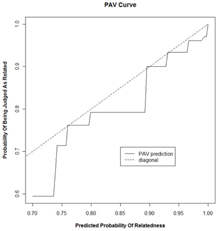
The maximum likelihood estimate of the probability that a pair is judged to be related given its predicted probability of relatedness. The curve is found using the PAV algorithm on data from 400 manually judged high-prob pairs and their probability of relatedness (equation 10).

Stem Evaluation

The Porter stemmer [2] is an algorithm that removes recognized suffixes from words to yield a putative root, or stem. Words that are stemmed to the same root word are presumed conflatable. That is, they may be used to refer to similar things, and hence they are candidates for query expansion. We evaluated this hypothesis directly by manually evaluating pairs of words having a common stem, and compared the results with the set of high-prob word pairs.

We randomly selected 1,000 distinct words from MEDLINE using a sampling probability proportional to their frequency. Each word was also required to have at least one other word with a common Porter stem, and was associated with that one with the highest MEDLINE frequency. The list of 1,000 word pairs was alphabetized by the first word, and each pair was examined to judge whether they possessed a common root.

Based on this manual evaluation, 63 pairs out of 1,000 were judged to not possess a common root. For example, the Porter stemmer identified unrelated pairs general/generated, and international/internal. Examples of word pairs judged to be related were cornea/corneas, and unilaterally/unilateral.

These judgments were then compared with the set of high-prob pairs, as described above. Within the 1,000 pairs, 792 were high-prob pairs and 208 low-prob pairs. Among the 792 high-prob pairs, 3.5% were judged unrelated. But among the 208 low-prob pairs, the error rate was more than four times this, at 16.8%. The Pearson chi-squared test for independence gives χ² = 49.32, with a negligible p-value. This confirms that the probability for pairs of words computed by equation (10) is indicative of semantic relatedness. It also suggests a potential method of filtering query expansions based on Porter stemming.

Probability Estimates Based on Lexsim Alone

Based on the processing of all 440 million token pairs with lexSim ≥ 0.5 where the w₄ trained weights are used, we can estimate the probability that a pair of token types are semantically related just from the value lexSim. This calculation is based on the assumption that when conSim = −1000 the pair is not semantically related. For all other pairs the probability is calculated based on the above lexSim slice analysis and the functions ${\left\{p_i\right\}}_{i=0}^{20}$. The composite curve for the probability of semantic relatedness is computed again by use of isotonic regression and the reasonable assumption that the probability should be a non-decreasing function of the lexSim score. The result is shown in Figure 6.

Figure 6.

Probability of semantic relatedness of a token type pair as a function of lexSim score. Applies only to pairs where lexSim ≥ 0.5.

An interesting aspect of Figure 6 is the observation that the predicted probabilities based on lexSim score alone are almost never as great as 0.7. This is to be compared with the fact that by making use of the context information available in conSim we are able to identify over 36 million token type pairs with a probability of being semantically related that is greater than or equal to 0.7 and this is just over 8% of the total of 440 million candidate token type pairs. Another point worth mentioning is the almost linear nature of the probability of semantic relatedness as a function of lexSim score. While linearity is not necessary for the slice analysis to work, linearity does seem desirable and perhaps provides a modicum of support for equations (4) and (5).

Discussion and Conclusion

There are several possible uses for the type of data produced by our analysis. Words semantically related to a query term or terms typed by a search engine user can provide a useful query expansion in either an automatic mode or with the user selecting from a displayed list of options for query expansion. Many missspellings occur in the literature and are disambiguated in the token pairs produced by the analysis. They can be recognized as closely related low frequency-high frequency pairs. They may allow better curation of the literature on the one hand or improved spelling correction of users queries on the other. In the area of more typical language analysis, a large repository of semantically related pairs can contribute to semantic tagging of text and ultimately to better performance on the semantic aspects of parsing. Also the material we have produced can serve as a rich source of morphological information. For example, inflectional and derivational transformations applicable to the technical language of biology are well represented in the data.

There is the possibility of improving on the methods we have used, while still applying the general approach. Either a more sensitive conSim or lexSim measure or both could lead to superior results. Undoubtedly conSim is limited by the fact that tokens in text follow a Zipfian [33] frequency distribution and most tokens appear infrequently. A pair of tokens that each appears infrequently have a decreased chance of encountering the same contextual tokens even when such an encounter would be appropriate to their meaning. This limits the effectiveness of conSim and we believe accounts for only being able to extract 8% of the 440 million token type pairs at a probability of semantic relatedness ≥ 0.7. There is probably no cure for this issue other than a larger corpus, which would be expected to yield a larger set of such high probability pairs (but perhaps not a fraction higher than 8%). While it is unclear to us how conSim might be structurally improved, it seems there is more potential with lexSim. lexSim treats features as basically independent contributors to the similarity of token types and this is not ideal. For example the feature ‘hiv’ usually refers to the human immunodeficiency virus. However, if ‘ive’ is also a feature of the token we may well be dealing with the word ‘hive’ which has no relation to a human immunodeficiency virus. Thus a more complicated model of the lexical similarity of strings could result in improved recognition of semantically related strings.

In future work we hope to investigate the application of the approach we have developed to multi-token terms. We also hope to investigate the possibility of more sensitive lexSim measures for improved performance. The current best lexSim weights are based on the machine learning method we present in this paper. It is possible that other methods of machine learning can also be used to bootstrap improved weights and such methods need to be investigated.

References

- 1.Jurafsky D, Martin JH. Speech and Language Processing. Upper Saddle River; New Jersey: Prentice Hall: 2000. [Google Scholar]
- 2.Porter MF. An algorithm for suffix stripping. Program. 1980;14(3):130–137. [Google Scholar]
- 3.Freitag D. Morphology Induction From Term Clusters. 9th Conference on Computational Natural Language Learning (CoNLL); Ann Arbor, Michigan: Association for Computational Linguistics; 2005. [Google Scholar]
- 4.Hammarström H, Borin L. Unsupervised Learning of Morphology. Computational Linguistics. 2011;37(2):309–350. [Google Scholar]
- 5.Kim YB, Graça J, Snyder B. EMNLP. Scotland, UK: ACL; 2011. Universal Morphological Analysis using Structured Nearest Neighbor Prediction; pp. 322–332. [Google Scholar]
- 6.Monson C. A framework for unsupervised natural language morphology induction. Proceedings of the ACL 2004 on Student research workshop; Barcelona, Spain: Association for Computational Linguistics; 2004. [Google Scholar]
- 7.Poon H, Cherry C, Toutanova K. NAACL-HLT. Boulder, Colorado: ACL; 2009. Unsupervised Morphological Segmentation with Log-Linear Models; pp. 209–217. [Google Scholar]
- 8.Schone P, Jurafsky D. Knowledge-free induction of morphology using latent semantic analysis. Proceedings of the 2nd workshop on Learning language in logic and the 4th conference on Computational natural language learning; Lisbon, Portugal: Association for Computational Linguistics; 2000. [Google Scholar]
- 9.Sirts K, Alumäe T. NAACL-HLT. Montreal, Canada: ACL; 2012. A Hierarchical Dirichlet Process Model for Joint Part-of-Speech and Morphology Induction; pp. 407–416. [Google Scholar]
- 10.Wicentowski R. SIGPHON. Barcelona, Spain: Association for Computational Linguistics; 2004. Multilingual Noise-Robust Supervised Morphological Analysis using the WordFrame Model. [Google Scholar]
- 11.Yarowsky D, Wicentowski R. Association for Computational Linguistics (ACL '00) Hong Kong: ACL; 2000. Minimally supervised morphological analysis by multimodal alignment; pp. 207–216. [Google Scholar]
- 12.Zhao Q, Marcus M. Long-Tail Distributions and Unsupervised Learning of Morphology. COLING, Mumbai, India. 2012:3121–3136. [Google Scholar]
- 13.Lazaridou A, Marelli M, Zamparelli R, Baroni M. Compositionally Derived Representations of Morphologically Complex Words in Distributional Semantics. 51st Annual Meeting of the Association for Computational Linguistics; Sofia, Bulgaria. ACL; 2013. pp. 1517–1526. [Google Scholar]
- 14.Luong T, Socher R, Manning C. Better Word Representations with Recursive Neural Networks for Morphology. Seventeenth Conference on Computational Natural Language Learning; Sofia, Bulgaria. ACL; 2013. pp. 104–113. [Google Scholar]
- 15.Means RW, Nemat-Nasser SC, Fan AT, Hecht-Nielsen R. A Powerful and General Approach to Context Exploitation in Natural Language Processing. HLT-NAACL 2004: Workshop on Computational Lexical Semantics; Boston, Massachusetts, USA: Association for Computational Linguistics; 2004. [Google Scholar]
- 16.Alberga CN. String similarity and misspellings. Communications of the ACM. 1967;10(5):302–313. [Google Scholar]
- 17.Findler NV, Leeuwen JV. A family of similarity measures between two strings. IEEE Transactions on Pattern Analysis and Machine Intelligence. 1979;PAMI-1(1):116–119. doi: 10.1109/tpami.1979.4766885. [DOI] [PubMed] [Google Scholar]
- 18.Hall PA, Dowling GR. Approximate string matching. Computing Surveys. 1980;12(4):381–402. [Google Scholar]
- 19.Wilbur WJ, Kim W. Flexible phrase based query handling algorithms. Proceedings of the ASIST 2001 Annual Meeting; Washington, D.C.. Information Today, Inc; 2001. pp. 438–449. [Google Scholar]
- 20.Willett P. Document retrieval experiments using indexing vocabularies of varying size. II. Hashing, truncation, digram and trigram encoding of index terms. Journal of Documentation. 1979;35(4):296–305. [Google Scholar]
- 21.Zobel J, Dart P. Finding approximate matches in large lexicons. Software-Practice and Experience. 1995;25(3):331–345. [Google Scholar]
- 22.Adamson GW, Boreham J. The use of an association measure based on character structure to identify semantically related pairs of words and document titles. Information Storage and Retrieval. 1974;10:253–260. [Google Scholar]
- 23.Damashek M. Gauging similarity with n-grams: Language-independent categorization of text. Science. 1995;267:843–848. doi: 10.1126/science.267.5199.843. [DOI] [PubMed] [Google Scholar]
- 24.Wilbur WJ. Global term weights for document retrieval learned from TREC data. Journal of Information Science. 2001;27(5):303–310. [Google Scholar]
- 25.Witten IH, Moffat A, Bell TC. Managing Gigabytes. Second. San Francisco: Morgan-Kaufmann Publishers, Inc; 1999. [Google Scholar]
- 26.Wilbur WJ. Unsupervised Learning of the Morpho-Semantic Relationship in MEDLINE®. Workshop on BioNLP 2007, Prague, Czech Republic. 2007:201–208. [Google Scholar]
- 27.Smith L, Rindflesch T, Wilbur WJ. MedPost: A part of speech tagger for biomedical text. Bioinformatics. 2004;20:2320–2321. doi: 10.1093/bioinformatics/bth227. [DOI] [PubMed] [Google Scholar]
- 28.Sparck Jones K. A statistical interpretation of term specificity and its application in retrieval. The Journal of Documentation. 1972;28(1):11–21. [Google Scholar]
- 29.Nash SG, Nocedal J. A numerical study of the limited memory BFGS method and the truncated-Newton method for large scale optimization. SIAM Journal of Optimization. 1991;1(3):358–372. [Google Scholar]
- 30.Ayer M, Brunk HD, Ewing GM, Reid WT, Silverman E. An empirical distribution function for sampling with incomplete information. Annals of Mathematical Statistics. 1954;26:641–647. [Google Scholar]
- 31.Hardle W. Smoothing techniques: with implementation in S. New York: Springer-Verlag; 1991. [Google Scholar]
- 32.Wilbur WJ, Yeganova L, Kim W. The Synergy Between PAV and AdaBoost. Machine Learning. 2005;61:71–103. doi: 10.1007/s10994-005-1123-6. [DOI] [PMC free article] [PubMed] [Google Scholar]
- 33.Zipf GK. Human Behavior and the Principle of Least Effort. Reading, MA: Addison-Wesley Publishing Co; 1949. [Google Scholar]