Analyzing ion distributions around DNA

Abstract

We present a new method for analyzing ion, or molecule, distributions around helical nucleic acids and illustrate the approach by analyzing data derived from molecular dynamics simulations. The analysis is based on the use of curvilinear helicoidal coordinates and leads to highly localized ion densities compared to those obtained by simply superposing molecular dynamics snapshots in Cartesian space. The results identify highly populated and sequence-dependent regions where ions strongly interact with the nucleic and are coupled to its conformational fluctuations. The data from this approach is presented as ion populations or ion densities (in units of molarity) and can be analyzed in radial, angular and longitudinal coordinates using 1D or 2D graphics. It is also possible to regenerate 3D densities in Cartesian space. This approach makes it easy to understand and compare ion distributions and also allows the calculation of average ion populations in any desired zone surrounding a nucleic acid without requiring references to its constituent atoms. The method is illustrated using microsecond molecular dynamics simulations for two different DNA oligomers in the presence of 0.15 M potassium chloride. We discuss the results in terms of convergence, sequence-specific ion binding and coupling with DNA conformation.

INTRODUCTION

How ions interact with DNA and what role they may play in modulating the structure and interactions of the DNA double helix has been the subject of many experimental and theoretical studies recent years. In structural terms, monovalent ions have been the subject of controversy because they are difficult to distinguish from water molecules in crystallographic studies (1–4) (even at very high resolution, (5)) and they are also not amenable to nuclear magnetic resonance (NMR) investigations. Thus, how frequently ions bind to specific DNA sites is still open to question, although results using other ions, which are less biologically relevant, but easier to locate experimentally (such as thallium or ammonium which are both reasonable models for potassium cations) have shown that monovalent ions can bind both in the major groove (favoring GC-rich regions) and in narrow minor grooves (e.g. A-tracts) (6,7). Experimental efforts in this field continue to develop and the reader is referred to recent work using small-angle X-ray scattering (8) and so-called ‘ion counting’ spectroscopic approaches (9,10).

In view of the experimental difficulties, molecular dynamics (MD) simulations have been used to study ion binding for many years (11–18). Initially, such simulations were limited to a few nanoseconds. Ion penetration of the grooves, and, in particular, replacement of waters forming the minor groove spine in A-tracts, was observed and was instrumental in encouraging further studies, however the relatively slow diffusion of the ions made it difficult to obtain convergence (11,13,14,19).

Simulations reaching 50 ns also showed ion binding in the grooves and found that binding was more extensive for potassium than for sodium. It was however noted that during 50 ns, individual ions still only sampled roughly one-third of the simulation box, remaining clearly distinguishable from one another, in violation of the assumption of ergodicity. In an exceptionally long simulation for the time, Pérez et al. studied the so-called Dickerson–Drew dodecamer (dCGCGAATTCGCG) for 1 μs in the presence of neutralizing sodium ions. High affinity ion binding in the AATT minor groove was observed with residence times up to 15 ns (20). This study also found a correlation between sodium ion binding and minor groove narrowing, following up on an earlier controversy in this area surrounding the interpretation of crystallographic results (1,4).

When analyzing molecular simulation data, in addition to problems linked with convergence, there are questions as to how to best measure ion distributions. Deoxyribonucleic acid (DNA) is a flexible macromolecule that, given its helical conformation, deforms easily by bending, twisting and stretching on the timescale of MD simulations. Thus, while it is possible to generate an overview of ion distributions by superposing the instantaneous DNA conformations from successive ‘snapshots’ (typically spaced in time by 1 ps intervals), the overall motions of the double helix will necessarily lead to some ‘blurring’ of the distributions associated with ions that are strongly interacting with DNA. Alternatively, one can count ion contacts with specific atoms of DNA using a chosen distance cutoff. This gives good local information, but is not well adapted to ions positioned, or fluctuating, between clusters of atoms, and it is clearly not adapted to analyzing overall distributions.

We now propose a new approach to analyze the distribution of ions, or molecules, around DNA based on the use of a natural coordinate system for DNA, namely curvilinear helicoidal coordinates (CHC). Since our algorithm, Curves+, provides a method for obtaining the helical axis of any DNA conformation, it is relatively easy to extend this analysis to determine the positions of ions or molecules around DNA in terms of their location with respect to the helical axis (using the base pair positions to define steps along the molecule and the local position of the helical grooves). Making this choice implies that overall helical deformations including twisting, bending and stretching can be eliminated from the analysis of ion densities. It is then possible to plot ion distributions radially from the curvilinear helical axis (i.e. as a cylindrical distribution function), along the length of the helical axis, or around the (curvilinear) helical axis, either for the entire molecule or for any chosen zone. We can use this approach to calculate average ion populations or local concentrations close to any chosen part of the molecule and also analyze the convergence of the ion distributions as a function of the duration of the MD simulations. Lastly, by using a single, average DNA conformation, we can also map the helicoidal ion coordinates back into Cartesian space and obtain 3D density plots that do not suffer from the DNA conformational fluctuations in the same way as the simple Cartesian superposition of MD snapshots and, as discussed below, lead to strikingly clear ion distributions.

This paper describes how curvilinear helicoidal ion parameters are defined and calculated. We then apply the new method to analyze potassium ion (K⁺) and chlorine ion (Cl⁻) distributions around two different DNA oligomers that were simulated for 1 μs in aqueous solution with a physiological concentration of KCl. Although K⁺ ions are expected to bind more strongly to DNA than Na⁺ because of their weaker first hydration shell (15–17,21), the results presented here show sequence-specific ion binding sites with surprisingly high occupancies. The new method enables spatially-localized, time-averaged populations and the corresponding molar concentrations to be calculated. We show that 1, 2 and 3D graphs using the curvilinear helicoidal coordinates make it easy to understand the overall ion distributions.

The software used for this analysis, ‘Canion’, is freely available, along with the latest version of Curves+ and the necessary user guides, at the following site: http://bisi.ibcp.fr/tools/curves_plus/. We note that Canion can be used not only for analyzing data from MD simulations, but can also directly read density matrices derived from continuum approaches to modeling ion distributions (see, e.g. (22,23)). This makes it easy to compare such results with MD simulations using the curvilinear helicoidal coordinate system.

MATERIALS AND METHODS

DNA trajectories

We illustrate the ion analysis developed here using microsecond long molecular dynamics trajectories for two 18-mer oligomers belonging to the so-called ABC (Ascona B-DNA Consortium) database (24–26). Both oligomers are based on tetranucleotide repeats, respectively, AGCT and ATCG, flanked by GC ends to reduce fraying during the simulations. Their sequences are GCCTAGCTAGCTAGCTGC and GCGCATGCATGCATGCGC (where the tetranucleotide repeat used to refer to the oligomers has been underlined).

Each oligomer was simulated using the AMBER program suite (27) and with the current ABC protocol (24). This involves the parm99 force field (28,29) with the bsc0 modifications (30). The oligomers were simulated using periodic boundary conditions with a truncated octahedral cell and a solvent environment consisting of SPC/E water molecules (31) (with a minimum thickness of 10 Å around the solute), leading to 11 621 and 11 546 water molecules for AGCT and ATCG, respectively). The DNA net charge is neutralized with K⁺ ions and then KCl ion pairs are added to reach a concentration of 150 mM KCl. The ions were represented using Dang parameters (32). Counterions were initially placed at random, at least 5 Å from the solute and 3.5 Å from one another. Electrostatic interactions were treated with the particle mesh Ewald method (33), using a real-space cutoff of 9 Å and cubic B-spline interpolation onto a charge grid with a 1-Å spacing. Lennard–Jones interactions were truncated at 9 Å. The pair list was built with a buffer region and updated whenever a particle moved by more than 0.5 Å.

The oligomers were initially built with a canonical B-DNA conformation. Initial equilibration involved energy minimization of the solvent, followed by a slow thermalization. Production simulations were carried out using a 2 fs time step in an NPT ensemble. The length of chemical bonds involving hydrogen were restrained using SHAKE (34) and the Berendsen algorithm (35) was used to control the temperature and the pressure, with a coupling constant of 5 ps. Center of mass motion was removed every ps to limit the translational kinetic energy of the solute (36).

Both oligomers were simulated for a total of 1 μs and conformational snapshots were saved for analysis every 1 ps (leading to 10⁶ data sets per oligomer).

DNA conformational analysis

The DNA conformation and the ion distribution were analyzed directly from the AMBER trajectory output using Curves+ (37,38). In the case of DNA, this analysis yields a curvilinear helical axis, and a full set of helical, backbone and groove parameters that can subsequently be used to generate time series or time-averaged probability distributions using the program Canal. As discussed below, a new option ‘ions’ is now available in Curves+ that triggers the calculation of the position of ions, water molecules, or any desired solute atoms in the trajectory. This output can then be analyzed with the Canion utility program, which is freely available along with Curves+, Canal and other utility software (http://bisi.ibcp.fr/tools/curves_plus/).

Ion analysis technique

In order to describe the position of atoms or ions around a nucleic acid substrate (or belonging to the substrate itself), we have chosen to use coordinates based on the helical axis of the nucleic acid. The Supplementary Information to this article contains a detailed description of this procedure. Briefly, the overall helical axis in Curves+ is built from a set of helical axis systems consisting of vectors d₁, d₂ and d₃ centered at point γ. d₃ is the local helical axis and d₁d₂ are coupled to the helical twist of the molecule, d₁ , being linked to the long axis of the base pairs. For each ion (or atom), we search for the helical axis system where the ion lies in the d₁d₂ plane. If several such systems are found, we choose the one leading to the shortest distance between the helical axis reference point γ and the ion. This distance defines the radial coordinate R from the ion to the helical axis (see Figure 1). The distance of the point γ along the helical axis in units of base pair steps defines the coordinate D (i.e. D can vary continuously from 1 to N within an N bp segment) and, finally, the angle of the vector from γ to the ion defines an angle with respect to a vector d₁ which constitutes the angular coordinate A. Given the definition of d₁, A ≈ 90° corresponds to the center of the minor groove and A ≈ 270° corresponds to the center of the major groove for a canonical B-DNA.

Figure 1.

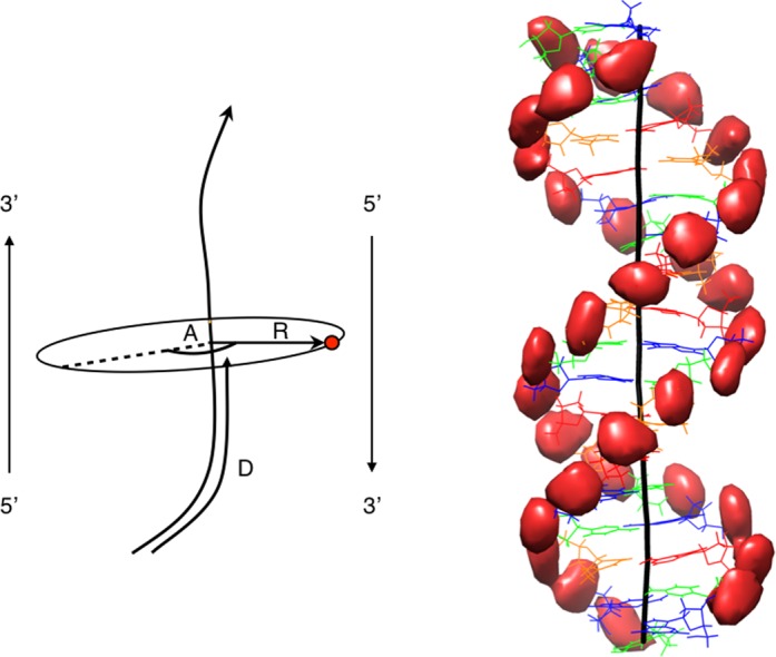
Left: Schematic view of the curvilinear helicoidal coordinates (CHC). An ion (red dot) is described by a distance D along the curved helical axis (black line), a radial distance R from the axis and an angle A from a reference vector which tracks the helical twist of the nucleic acid. At the base pair levels, this vector corresponds approximately to the long axis of the base pairs and points toward the 5′-3′ strand. Consequently, A ≈ 90° places an ion in the minor groove and A ≈ 270° places an ion in the major groove. Right: Isodensity surfaces (red) for the phosphorus atoms of the AGCT oligomer analyzed in the CHC system, then mapped into Cartesian space using the average helical axis of the oligomer (black line). The nucleotides are colored to indicate the base sequence (G: blue, C: green, A: red, T: orange). All isodensity plots were obtained using Chimera (39,40).

For a molecular dynamics trajectory (or an ensemble of experimental structures, such as that resulting from an NMR study), the ion analysis is performed on each snapshot (or experimental structure) using the corresponding helical axis and stored in a file. This file is then read by the Canion program and the ions positions are accumulated in a 3D histogram with a bin size in curvilinear helicoidal space of 0.5 Å in R, 1/6 of a base pair step (≈0.5 Å) in D and 5° in A. We then analyze the ion distributions in 1D (R, D or A), in 2D (RA, DA, DR) or in 3D Cartesian space (see below). Note that in the case of a 2D RA analysis, we use polar coordinate plots to make the results easier to understand. Ion distributions can be obtained for the entire space surrounding the oligomer, or for any selected zone, defined by fixing lower and upper limits on R, D or A. Note that, by default, we use an upper limit of R = 30 Å since beyond this point the solute molecule has little impact on the ion distribution and the helicoidal coordinate analysis ceases to be of interest.

For any chosen spatial region, we can obtain the time-averaged ion populations. However, it is also useful to be able to calculate ion densities, or more specifically molarities. (Note densities in ions.Å⁻³ can be converted to molarities by dividing by N_A/10²⁷ = 6.022 × 10⁻⁴, where 10²⁷ is the number of cubic angstroms per liter and N_A is Avogadro's number.) Since the volumes of the histogram bins in CHC change as a function of R and, if the helical axis is curved, also as a function of A at each base pair step, it is necessary to calculate the Cartesian volume for each element of the CHC histogram. Note also that curved helical axes impose limits on the radial distance at which curvilinear helicoidal coordinates can be calculated. See the Supplementary Information for details of these calculations.

In order to recreate a 3D Cartesian space distribution, the helicoidal ion coordinates can be mapped back to Cartesian space with respect to a chosen helical axis, with typical choices being the axis of the average nucleic acid structure from the corresponding molecular dynamics trajectory, or a linear axis corresponding to a regular helix with user-defined twist and rise.

Lastly, when calculating ion densities close to DNA, it seems reasonable to exclude the volume occupied by the solute molecule itself. This has been made possible in the Canion program by determining which CHC volume elements lie inside the van der Waals envelope of the solute molecule (using standard Pauling values, P: 1.9 Å, C: 1.6 Å, N: 1.5 Å, O: 1.4 Å, H: 1.2 Å). While taking the solute excluded volume into account is optional in the Canion program, it is particularly useful when comparing the ion molarities in the two grooves of helical nucleic acids, and this option has been selected in all the results presented here.

RESULTS AND DISCUSSION

Before discussing the ion distributions around the AGCT and ATGC oligomers, we can first ask whether using the CHC system is in fact helpful. To test this we will use the phosphorus atoms belonging to the AGCT oligomer as an example.

We start by recording the position of each of these atoms from every 1 ps snapshot along the 1 μs trajectory, using the curvilinear helicoidal coordinates defined in the methodology section. Each phosphorus atom is described by its radial R, longitudinal D and angular A coordinates (see Figure 1). This implies that the most significant overall fluctuations of the oligomer (stretching, twisting and bending) will not affect the helicoidal coordinates describing its constituent atoms. To test this, we first generate an average DNA structure from the trajectory. We then calculate its helical axis with Curves+ (37) and use it to convert the instantaneous helicoidal coordinates of the phosphorus atoms from each snapshot to a common Cartesian coordinate system. The scatter in the positions of each phosphorus atom can then be used to generate the isodensity surfaces shown on the right of Figure 1 (plotted using Chimera (39,40)). More quantitatively, we can calculate root mean square fluctuations (RMSF) for each phosphorus atom and compare the values with those obtained by simply superposing the Cartesian coordinates from each snapshot. The results in Figure 2 show that the CHC method leads to smaller RMSF values in almost all cases. This reduction is particularly interesting in the center of each strand, where the overall fluctuations of the oligomer might not have been expected to have a significant effect.

Figure 2.

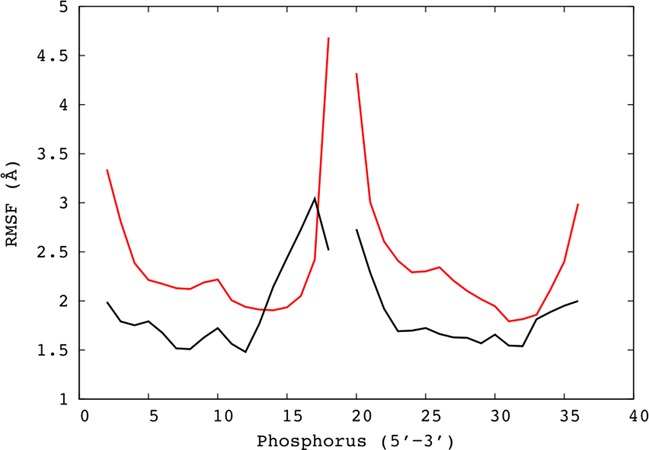
Root mean square fluctuations (Å) for the phosphorus atoms of the AGCT oligomer are smaller when calculated using the CHC analysis mapped into Cartesian space (black lines), than when simply superposing snapshots from the molecular dynamics simulation (red lines). Note that phosphates belonging to the two strands are shown consecutively in the 5′-3′ direction.

Analyzing the position of DNA atoms in helicoidal coordinates is also useful for providing reference positions to help in analyzing ion distributions. This is illustrated in Figure 3 where we plot the phosphorus distributions in helicoidal coordinate space using the three possible 2D plots: DA (top left), DR (top right) and RA (bottom left). The DA plot (obtained by summing the phosphorus density over all radial distances R) shows an ‘unwrapped’ and ‘unwound’ view of the oligomer. The phosphate densities of each strand consequently lead to a column of distributions at constant A values, with the smaller separation between the two columns corresponding to the minor groove of the double helix. In the DR plot (obtained by summing over all angles A), all the phosphorus atoms are seen to lie at constant distance (R = 10.25 Å) from the helical axis. This distance can be used to define a useful radius delimiting the helical grooves, as shown by the white circle in the RA plot (obtained by summing over all axial distances D). Here, all the phosphorus atom distributions are superposed and closely follow the R = 10.25 Å radius circle.

Figure 3.

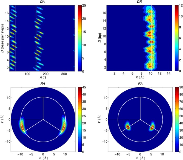
Average phosphorus distributions calculated using CHC for the 1 μs AGCT trajectory and plotted in various planes: DA (top left), DR (top right), RA (bottom left). The bottom right plot shows the RA plane for the sugar C1′ atoms from the same trajectory. The blue to red color scale represents increasing molarity. DR and RA plots show the average radius of the phosphorus atoms from the helical axis as a white line and as a white circle, respectively. The DA and RA plots show the minor groove limits, defined by the average C1′ positions, as a white line and as white radial vectors, respectively. RA plots also have a vertical radial vector indicating the center of the major groove.

Figure 3 contains one further plot (bottom right) corresponding to an RA analysis of the sugar C1′ atoms. These atoms constitute a useful guide to the position of the minor groove since they reflect the position of the glycosidic bonds. Note that the C1′ densities are tighter than those of the phosphorus atoms, since they are less affected by backbone fluctuations, but also because, being closer to the helical axis, they are affected less by effectively unwinding the B-DNA helix in the helicoidal coordinate space (an effect more visible for the more distant phosphorus atoms in the DA and RA plots). Drawing radial vectors through the center of the C1′ distributions enables us to define the minor groove as lying between A values of 33° and 147°. We take remaining values of A to belong to the major groove, since we do not attribute regions specifically to the phosphodiester backbones. We complete the visual reference system in RA plots by adding a line along the external bisector of the C1′ vectors to indicate the center of the major groove. Note that the C1′ vectors can also be used to show the minor groove position in 1D A plots (where they become vertical lines) and, similarly, the phosphorus radius can be added as a vertical line in 1D R plots (see below).

We should remark that the usefulness of CHC approach depends on having a well-defined helical axis. Curves+ calculates a curvilinear axis that runs between the terminal base pairs of the oligomer. However, if significant end-fraying occurs, this can lead to perturbations of the axis which will then be reflected in the helicoidal coordinates used to describe atomic (or ionic) positions. In addition, the position of ions beyond the ends of the helical axis will not be recorded.

Before proceeding with the analysis of ion distributions around DNA, we need to consider the question of convergence. As shown below, the main ion densities occur in the DNA grooves (R ≤ 10.25 Å) and between successive base pairs (defined here as N − 0.2 ≤ D ≤ N + 1.2 for a base pair step N_pN + 1). We have therefore tested convergence by looking at the average potassium ion populations as a function of time for unique base pair steps belonging to the central tetranucleotide and in the associated major or minor grooves. The results for the AGCT oligomer are shown in Figure 4 and the corresponding data for ATGC in Supplementary Figure S4. Both these figures show that at least 300 ns of simulation are necessary to achieve stable ion populations (and, in some cases, non-negligible changes can occur up to 500 ns).

Figure 4.

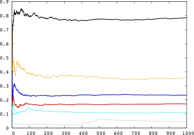
Time-averaged K⁺ populations within the DNA grooves for the unique base pair steps (T8pA9, A9pG10, G10pC11) belonging to the central tetranucleotide of the AGCT oligomer for increasing durations (ns) of the molecular dynamics trajectory.

A second test of convergence is shown in Figure 5, where we have simply generated average Cartesian coordinates for the AGCT oligomer using 1 ps snapshots and including the position of all the K⁺ (blue) and Cl⁻ (green) ions. When the average is made over a few tens of nanoseconds of simulation, the ions tend to sample limited volumes of the simulation cell (15) and are thus clearly distinguishable. However, after 1 μs of simulation the average ion positions all coincide at the origin of the simulation cell, showing they have had time to thoroughly sample the full simulation cell in an equivalent manner, satisfying the principle of ergodicity.

Figure 5.

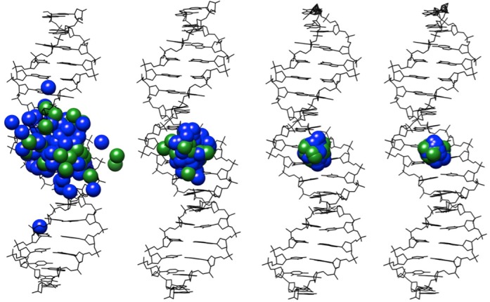
Averaged conformation of the AGCT oligomer (black line drawing) and the associated average locations of the K⁺ (blue spheres) and Cl⁻ (green spheres) ions calculated for increasing durations of the molecular dynamics trajectory.

Having shown that reasonable convergence has been achieved, we turn to an overall analysis of the potassium ion distributions around the AGCT oligomer. We begin with 1D R, D and A plots shown in Figure 6. The radial distance R plot, that is also a radial distribution function, shows two peaks within the grooves and one beyond the phosphorus atom radius (indicated by the vertical line). Note that the maximum molarity for the peak closest to the helical axis reaches almost 14 times the bulk value, whereas, at 30 Å the value has fallen slightly below the effective bulk molarity (0.336 M, taking into account the extra K⁺ ions added to achieve neutrality). The axis distance D plot shows two interesting features: first, three repeated profiles that are in register with the repeating base sequence and which show strong molarity peaks at three consecutive GpC steps; second, a decrease in ion density toward the ends of the oligomer, reflecting the decreasing phosphate density (41). Lastly, the angular A plot shows that potassium ion density peaks occur in both grooves.

Figure 6.

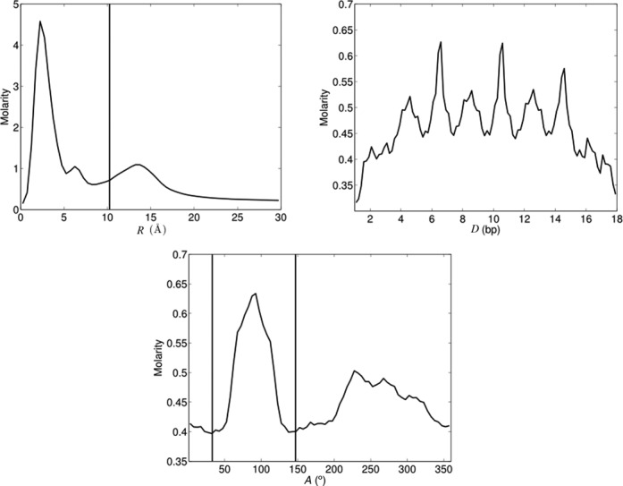
1D K⁺ distributions averaged over the 1 μs AGCT trajectory. The vertical line in the R plot indicates the radial position of the phosphorus atoms, while the shorter distance between the two vertical lines in the A plot delimits the minor groove using the angular position of the sugar C1′ atoms (see Figure 3).

We can further refine this analysis by passing to 2D representations. Figure 7 shows the DA and RA plots for potassium ions, again around the AGCT oligomer (with radial sampling limited to 15 Å). This enables us to identify the R peak closest to the helical axis (seen in Figure 6) as ion binding in the center of the major groove, while on the minor groove side there is a more diffuse density with two maxima (see the DA and RA plots). Before filling in the details of the potassium ion distributions, it is worth contrasting these results with those for the chlorine anions. Supplementary Figure S5 shows that chlorine anions have almost no density within the phosphorus radius, although they begin to penetrate when the phosphate density decreases toward the ends of the oligomer (see the DR plot). As expected, this penetration mainly occurs on the side of the wider major groove (see the RA plot).

Figure 7.

2D K⁺ distributions averaged over the 1 μs AGCT trajectory: DA plane (top left), DR plane (top right), RA plane (bottom). The results are plotted as molarities as shown by the color bars, with a blue to red scale indicating increasing values.

In order to complete the potassium ion analysis, it is useful to look at the 3D ion distributions reconstructed from the instantaneous helicoidal coordinates using a single, average helical axis (as for the RMSF calculations in Figure 2). These distributions are shown as isodensity plots in Figure 8. The left image shows the average DNA conformation as a wire diagram with K⁺ ion distributions at two isodensity levels: 15 M (red solid volumes) and 5 M (green mesh). The right image shows the same isodensities, but with a surface view of DNA that helps to locate the ions within the major and minor grooves. As already seen in Figure 4, the largest ion densities occur in the major groove of the GpC steps, whereas the largest minor groove densities occur at TpA steps.

Figure 8.

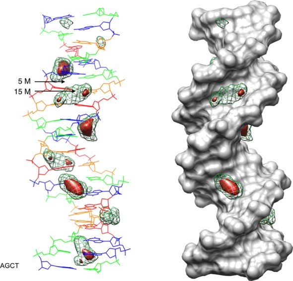
3D K⁺ distributions obtained by mapping CHC analysis of the 1 μs AGCT trajectory into Cartesian space with respect to the average DNA structure, shown as a line drawing on the left (G: blue, C: green, A: red, T: orange) and as a gray solvent accessible surface on the right. Molarity isodensity surfaces for potassium ions are plotted at 15 M (solid red) and 5 M (green mesh).

At this stage, it is useful to compare the AGCT oligomer with the results obtained for the ATGC sequence. Although the latter oligomer has a similar overall B-DNA structure and the same 50/50 balance of AT and GC base pairs, its ion distribution is rather different as shown by the 3D images in Supplementary Figure S6. Using the same isodensity surfaces as Figure 8 makes it clear that local K⁺ densities occupy smaller volumes in both grooves. In the major groove, they are again localized at GpC, while in the minor groove the densities are considerably weaker and associated with ApT steps.

Using the 3D information we can now return to 2D RA plots for a detailed and quantitative analysis for individual base pair steps and for each groove. Figure 9 shows the results for unique base pair steps of the central tetranucleotide of each oligomer: TpA, ApG and GpC for the AGCT oligomer and ApT, TpG and GpC for the ATGC oligomer. In each case, the average ion populations within the grooves are shown (corresponding to the data already plotted in Figure 4). It is striking that GpC steps in the AGCT oligomer have potassium ions strongly localized in their major grooves almost 80% of the time. This value decreases somewhat, but still exceeds 60%, for the same step in the ATGC oligomer. These main ion-binding sites lead to local molarities above 50 M, almost 150 times higher than the bulk potassium ion concentrations. Secondary ion binding sites, occupied roughly 25–35% of the time, occur in the minor groove of TpA steps and the major groove of ApG steps for AGCT, and also in the major grooves of ApT and TpG steps for ATGC.

Figure 9.

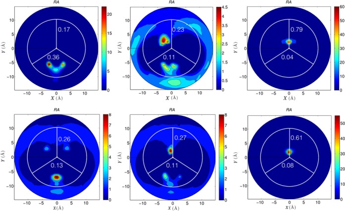
2D RA K⁺ distributions for various dinucleotide steps within the central tetranucleotides of the AGCT and ATGC oligomers, averaged over the corresponding 1 μs trajectories. The blue to red color scale indicates increasing molarity values. In each plot, the numbers in the upper and lower semicircles indicate the average K⁺ occupancy in the major and minor grooves, respectively.

Finally, we consider the question of whether cation binding within the grooves of DNA is related to fluctuations in groove width. This question has been the subject of extensive discussions (1,4,12,15,20), it being argued that bound cations should be able to counteract phosphate repulsion and lead to groove narrowing. Conclusions were however unclear, in part because it was difficult to define what ‘being within the grooves’ meant from a geometrical point of view. We can now revisit this question in the light of the CHC ion analysis. For this, we have added the groove width variations to the 1D axis distance D plots of K⁺ ion density, where the summation over R has now been limited to the grooves (R = 0–10.25 Å) and the summation of the angles A has been limited to either the minor or major groove. Figure 10 shows the results for AGCT oligomer. For this case, there is a clear oscillation of both groove widths (dotted lines), in register with the tetranucleotide repeating sequence. This oscillation is related to peaks in the ion density, but note that the grooves are wide when the ion density in the grooves is high. These findings are contradictory to an argument based on groove narrowing due to the compensation of phosphate repulsion. In the ATGC oligomer (see Supplementary Figure S7), the groove widths vary significantly less along the sequence (other than at the ends of the oligomer), but again there is no indication that ion binding leads to groove narrowing. Confirming these findings will however require the study of a wider range of base sequences.

Figure 10.

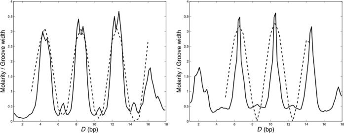
Variations in K⁺ molarity along the DNA grooves (solid lines) of the AGCT oligomer. Values are averaged over the 1 μs AGCT trajectory and compared with variations in groove width (dotted lines). Groove width variations are plotted in Å with respect to the respective minimal values (major: 10.0 Å, minor: 3.5 Å) on the same scale as the molarities. Left: major groove. Right: minor groove.

CONCLUSION

We propose a novel method for analyzing the distributions of ions or molecules (notably solvent molecules) around helical nucleic acids. By using curvilinear helicoidal coordinates to locate the particles we eliminate the ‘blurring’ of the distributions for ions whose movements are coupled to the large amplitude fluctuations of the double helix, notably bending, stretching and twisting. In addition, the helicoidal coordinates make it possible to calculate ion populations, or densities, in any zone surrounding the solute molecule. One can visualize the resulting ion distributions in helicoidal coordinates in 1D or 2D and also map the helicoidal coordinates back into Cartesian space to visualize 3D Cartesian space ion densities. Applying this technique to the analysis of 1 μs molecular dynamics trajectories of two DNA oligomers enables us to quantify the convergence of the ion distributions (which requires at least 300 ns of simulation) and to identify strongly localized, sequence-dependent ion binding sites (without requiring the use of distance cutoffs with respect to specific solute atoms). This analysis can be applied to any helical nucleic acid conformations (derived from molecular simulations or from experiment) and to any surrounding species such as ions, water molecules or ligands. The software necessary to carry out the analysis (Curves+ and associated utility programs) is freely available.

SUPPLEMENTARY DATA

Supplementary Data are available at NAR Online.

FUNDING

Centre National de la Recherche Scientifique (CNRS) and the Agence Natoinale de la Recherche (ANR) project CHROME [ANR-12_BSV5-0017-01 to R.L. and K.Z.]; Swiss National Science Foundation for funding under award 2000020_143613/1 (to J.H.M. and M.P.). Open access publication costs were covered by the project CHROME.

Conflict of interest statement. None declared.

REFERENCES

- 1.McFail-Isom L., Sines C.C., Williams L.D. DNA structure: cations in charge. Curr. Opin. Struct. Biol. 1999;9:298–304. doi: 10.1016/S0959-440X(99)80040-2. [DOI] [PubMed] [Google Scholar]
- 2.Tereshko V., Minasov G., Egli M. The Dickerson-Drew B-DNA dodecamer revisited at atomic resolution. J. Am. Chem. Soc. 1999;121:470–471. [Google Scholar]
- 3.Chiu T.K., Kaczor-Grzeskowiak M., Dickerson R.E. Absence of minor groove monovalent cations in the crosslinked dodecamer CGCGAATTCGCG. J. Mol. Biol. 1999;292:589–608. doi: 10.1006/jmbi.1999.3075. [DOI] [PubMed] [Google Scholar]
- 4.Hamelberg D., McFail-Isom L., Williams L.D., Wilson W.D. Flexible structure of DNA: ion dependence of minor-groove structure and dynamics. J. Am. Chem. Soc. 2000;122:10 513–10 520. [Google Scholar]
- 5.Maehigashi T., Hsiao C., Woods K.K., Moulaei T., Hud N.V., Williams L.D. B-DNA structure is intrinsically polymorphic: even at the level of base pair positions. Nucleic Acids Res. 2012;40:3714–3722. doi: 10.1093/nar/gkr1168. [DOI] [PMC free article] [PubMed] [Google Scholar]
- 6.Hud N.V., Sklenár V., Feigon J. Localization of ammonium ions in the minor groove of DNA duplexes in solution and the origin of DNA A-tract bending. J. Mol. Biol. 1999;286:651–660. doi: 10.1006/jmbi.1998.2513. [DOI] [PubMed] [Google Scholar]
- 7.Howerton S.B., Sines C.C., VanDerveer D., Williams L.D. Locating monovalent cations in the grooves of B-DNA. Biochemistry. 2001;40:10 023–10 031. doi: 10.1021/bi010391+. [DOI] [PubMed] [Google Scholar]
- 8.Pollack L. SAXS studies of ion-nucleic acid interactions. Annu. Rev. Biophys. 2011;40:225–242. doi: 10.1146/annurev-biophys-042910-155349. [DOI] [PubMed] [Google Scholar]
- 9.Bai Y., Greenfeld M., Travers K.J., Chu V.B., Lipfert J., Doniach S., Herschlag D. Quantitative and comprehensive decomposition of the ion atmosphere around nucleic acids. J. Am. Chem. Soc. 2007;129:14 981–14 988. doi: 10.1021/ja075020g. [DOI] [PMC free article] [PubMed] [Google Scholar]
- 10.Lipfert J., Doniach S., Das R., Herschlag D. Understanding nucleic acid-ion interactions. Annu. Rev. Biochem. 2014;83 doi: 10.1146/annurev-biochem-060409-092720. ch.19. (advance publication) [DOI] [PMC free article] [PubMed] [Google Scholar]
- 11.Young M.A., Jayaram B., Beveridge D.L. Intrusion of counterions into the spine of hydration in the minor groove of B-DNA: fractional occupancy of electronegative pockets. J. Am. Chem. Soc. 1997;119:59–69. [Google Scholar]
- 12.McConnell K.J., Beveridge D.L. DNA structure: what's in charge. J. Mol. Biol. 2000;304:803–820. doi: 10.1006/jmbi.2000.4167. [DOI] [PubMed] [Google Scholar]
- 13.Auffinger P., Westhof E. Water and ion binding around RNA and DNA (C,G) oligomers. J. Mol. Biol. 2000;300:1113–1131. doi: 10.1006/jmbi.2000.3894. [DOI] [PubMed] [Google Scholar]
- 14.Rueda M., Cubero E., Laughton C.A., Orozco M. Exploring the counterion atmosphere around DNA: what can be learned from molecular dynamics simulations. Biophys. J. 2004;87:800–811. doi: 10.1529/biophysj.104.040451. [DOI] [PMC free article] [PubMed] [Google Scholar]
- 15.Várnai P., Zakrzewska K. DNA and its counterions: a molecular dynamics study. Nucleic Acids Res. 2004;32:4269–4280. doi: 10.1093/nar/gkh765. [DOI] [PMC free article] [PubMed] [Google Scholar]
- 16.Cheng Y.H., Korolev N., Nordenskiold L. Similarities and differences in interaction of K+ and Na+ with condensed ordered DNA. A molecular dynamics computer simulation study. Nucleic Acids Res. 2006;34:686–696. doi: 10.1093/nar/gkj434. [DOI] [PMC free article] [PubMed] [Google Scholar]
- 17.Dixit S.B., Mezei M., Beveridge D.L. Studies of base pair sequence effects on DNA solvation based on all-atom molecular dynamics simulations. J. Biosci. 2012;37:399–421. doi: 10.1007/s12038-012-9223-5. [DOI] [PubMed] [Google Scholar]
- 18.Mocci F., Laaksonen A. Insight into nucleic acid counterion interactions from inside molecular dynamics simulations is “worth its salt”. Soft Matter. 2012;8:9268–9284. [Google Scholar]
- 19.Min D.H., Li H.Z., Li G.H., Berg B.A., Fenley M.O., Yang W. Efficient sampling of ion motions in molecular dynamics simulations on DNA: variant Hamiltonian replica exchange method. Chem. Phys. Lett. 2008;454:391–395. [Google Scholar]
- 20.Pérez A., Luque F.J., Orozco M. Dynamics of B-DNA on the microsecond time scale. J. Am. Chem. Soc. 2007;129:14 739–14 745. doi: 10.1021/ja0753546. [DOI] [PubMed] [Google Scholar]
- 21.Mezei M., Beveridge D.L. Monte Carlo studies of the structure of dilute aqueous sclutions of Li+, Na+, K+, F-, and Cl- J. Chem. Phys. 1981;74:6902–6910. [Google Scholar]
- 22.Howard J.J., Lynch G.C., Pettitt B.M. Ion and solvent density distributions around canonical B-DNA from integral equations. J. Phys. Chem. B. 2011;115:547–556. doi: 10.1021/jp107383s. [DOI] [PMC free article] [PubMed] [Google Scholar]
- 23.Giambaşu G.M., Luchko T., Herschlag D., York D.M., Case D.A. Ion counting from explicit-solvent simulations and 3D-RISM. Biophys. J. 2014;106:883–894. doi: 10.1016/j.bpj.2014.01.021. [DOI] [PMC free article] [PubMed] [Google Scholar]
- 24.Lavery R., Zakrzewska K., Beveridge D., Bishop T.C., Case D.A., Cheatham T., Dixit S., Jayaram B., Lankas F., et al. A systematic molecular dynamics study of nearest-neighbor effects on base pair and base pair step conformations and fluctuations in B-DNA. Nucleic Acids Res. 2010;38:299–313. doi: 10.1093/nar/gkp834. [DOI] [PMC free article] [PubMed] [Google Scholar]
- 25.Dixit S.B., Beveridge D.L., Case D.A., Cheatham T.E.3., Giudice E., Lankas F., Lavery R., Maddocks J.H., Osman R., et al. Molecular dynamics simulations of the 136 unique tetranucleotide sequences of DNA oligonucleotides. II: sequence context effects on the dynamical structures of the 10 unique dinucleotide steps. Biophys. J. 2005;89:3721–3740. doi: 10.1529/biophysj.105.067397. [DOI] [PMC free article] [PubMed] [Google Scholar]
- 26.Beveridge D.L., Barreiro G., Byun K.S., Case D.A., Cheatham T.E.3., Dixit S.B., Giudice E., Lankas F., Lavery R., et al. Molecular dynamics simulations of the 136 unique tetranucleotide sequences of DNA oligonucleotides. I. Research design and results on d(CpG) steps. Biophys. J. 2004;87:3799–3813. doi: 10.1529/biophysj.104.045252. [DOI] [PMC free article] [PubMed] [Google Scholar]
- 27.Pearlman D.A., Case D.A., Caldwell J.W., Ross W.S., Cheatham T.E., DeBolt S., Ferguson D., Seibel G., Kollman P. AMBER, a package of computer programs for applying molecular mechanics, normal mode analysis, molecular dynamics and free energy calculations to simulate the structural and energetic properties of molecules. Comput. Phys. Commun. 1995;91:1–41. [Google Scholar]
- 28.Cheatham T.E.3., Cieplak P., Kollman P.A. A modified version of the Cornell et al. force field with improved sugar pucker phases and helical repeat. J. Biomol. Struct. Dyn. 1999;16:845–862. doi: 10.1080/07391102.1999.10508297. [DOI] [PubMed] [Google Scholar]
- 29.Case D.A., Cheatham T.E., Darden T., Gohlke H., Luo R., Merz K.M., Onufriev A., Simmerling C., Wang B., Woods R.J. The Amber biomolecular simulation programs. J. Comput. Chem. 2005;26:1668–1688. doi: 10.1002/jcc.20290. [DOI] [PMC free article] [PubMed] [Google Scholar]
- 30.Pérez A., Marchán I., Svozil D., Sponer J., Cheatham T.E., Laughton C.A., Orozco M. Refinement of the AMBER force field for nucleic acids: improving the description of alpha/gamma conformers. Biophys. J. 2007;92:3817–3829. doi: 10.1529/biophysj.106.097782. [DOI] [PMC free article] [PubMed] [Google Scholar]
- 31.Berendsen H.J.C., Grigera J.R., Straatsma T.P. The missing term in effective pair potentials. J. Phys. Chem. 1987;91:6269–6271. [Google Scholar]
- 32.Dang L.X. Mechanism and thermodynamics of ion selectivity in aqueous-solutions of 18-crown-6 ether - A molecular dynamics study. J. Am. Chem. Soc. 1995;117:6954–6960. [Google Scholar]
- 33.Essmann U., Perera L., Berkowitz M.L., Darden T., Lee H., Pedersen L.G. A smooth particle mesh Ewald method. J. Chem. Phys. 1995;103:8577–8593. [Google Scholar]
- 34.Ryckaert J.P., Ciccotti G., Berendsen H.J.C. Numerical-integration of Cartesian equations of motion of a system with constraints - molecular-dynamics of N-Alkanes. J. Comput. Phys. 1977;23:327–341. [Google Scholar]
- 35.Berendsen H.J.C., Postma J.P.M., van Gunsteren W.F., DiNola A., Haak J.R. Molecular dynamics with coupling to an external bath. J. Chem. Phys. 1984;81:3684–3690. [Google Scholar]
- 36.Harvey S.C., Tan R.K.Z., Cheatham T.E., III The flying ice cube: velocity rescaling in molecular dynamics leads to violation of energy equipartition. J. Comput. Chem. 1998;19:726–740. [Google Scholar]
- 37.Lavery R., Moakher M., Maddocks J.H., Petkeviciute D., Zakrzewska K. Conformational analysis of nucleic acids revisited: Curves+ Nucleic Acids Res. 2009;37:5917–5929. doi: 10.1093/nar/gkp608. [DOI] [PMC free article] [PubMed] [Google Scholar]
- 38.Blanchet C., Pasi M., Zakrzewska K., Lavery R. CURVES+ web server for analyzing and visualizing the helical, backbone and groove parameters of nucleic acid structures. Nucleic Acids Res. 2011;39:W68-W73. doi: 10.1093/nar/gkr316. [DOI] [PMC free article] [PubMed] [Google Scholar]
- 39.Pettersen E.F., Goddard T.D., Huang C.C., Couch G.S., Greenblatt D.M., Meng E.C., Ferrin T.E. UCSF Chimera–a visualization system for exploratory research and analysis. J. Comput. Chem. 2004;25:1605–1612. doi: 10.1002/jcc.20084. [DOI] [PubMed] [Google Scholar]
- 40.Goddard T.D., Huang C.C., Ferrin T.E. Visualizing density maps with UCSF Chimera. J. Struct. Biol. 2007;157:281–287. doi: 10.1016/j.jsb.2006.06.010. [DOI] [PubMed] [Google Scholar]
- 41.Stein V.M., Bond J.P., Capp M.W., Anderson C.F., Record M.T., Jr Importance of coulombic end effects on cation accumulation near oligoelectrolyte B-DNA: a demonstration using 23Na NMR. Biophys. J. 1995;68:1063–1072. doi: 10.1016/S0006-3495(95)80281-X. [DOI] [PMC free article] [PubMed] [Google Scholar]
Associated Data
This section collects any data citations, data availability statements, or supplementary materials included in this article.