Advanced CLARITY for rapid and high-resolution imaging of intact tissues

Abstract

CLARITY is a method for chemical transformation of intact biological tissues into a hydrogel-tissue hybrid, which becomes amenable to interrogation with light and macromolecular labels while retaining fine structure and native biological molecules. This emerging accessibility of information from large intact samples has created both new opportunities and new challenges. Here we describe next-generation protocols spanning multiple dimensions of the CLARITY workflow, ranging from a novel approach to simple, reliable, and efficient lipid removal without electrophoretic instrumentation (passive CLARITY), to optimized objectives and integration with light-sheet optics (CLARITY-optimized light-sheet microscopy or COLM) for accelerating data collection from clarified samples by several orders of magnitude while maintaining or increasing quality and resolution. These methods may find application in the structural and molecular analysis of large assembled biological systems such as the intact mammalian brain.

Introduction

One goal of modern neuroscience is to map the architecture of neural circuits with both high (wiring-level) resolution and broad (brainwide) perspective. This challenge has drawn the attention of generations of scientists, beginning with Cajal’s detailed representations of neurons visualized at high resolution with the Golgi staining technique while still embedded within semi-intact brain tissue. Principles fundamental to the understanding of neural systems can result from such an integrative approach, but while progress has been made, many challenges and opportunities remain.

Over the last few decades, electron microscopy (EM) has emerged as a foundational method for deciphering details of neuronal circuit structure^1,2. The key advantage of EM in this regard (relative to light microscopy) is identification of presynaptic active zones containing neurotransmitter vesicles apposed to postsynaptic structures. In addition, EM facilitates visualization of some of the very finest branches of axons. However, EM tissue mapping requires relatively slow steps involving ultrathin sectioning/ablation and reconstruction; most importantly, the sample contrast preparation is largely incompatible with rich molecular phenotyping that could provide critical information on cell and synapse type. Ideally, datasets resulting from intact-brain mapping should be linkable to molecular information on the types of cells and synapses that are imaged structurally, and even to dynamical information on natural activity pattern history (in these same circuits) known to be causally relevant to animal behavior. Suitable light-based imaging approaches, combined with specific genetic or histochemical molecular labeling methods, have emerged as important tools to visualize the structural, molecular and functional architecture of biological tissues, with a particularly vital role to play in emerging brainwide, high-resolution neuroanatomy.

Confocal methods revolutionized light microscopy by enabling optical sectioning in thick (tens of micrometers) fluorescently-labeled samples, thereby allowing 3D reconstruction without the need for ultrathin physical sectioning³. Two-photon microscopy further increased the accessible imaging depth (to hundreds of micrometers) even in living tissue samples⁴, and adaptive-optics approaches have improved imaging depth further⁵. However, light microscopy remains limited for imaging throughout intact vertebrate nervous systems (for example, mouse brains span many millimeters even in the shortest spatial dimension, and are opaque on this scale due chiefly to light scattering). A common work-around to this limitation has been to slice brains into thin sections, in manual or automated fashion, followed by confocal or two-photon imaging^6,7; however, detailed labeling and reconstruction from thin sections has been (so far) limited to small volumes of tissue. An ideal integrative approach would be to label and image entirely intact vertebrate brains at high resolution.

As a step in this direction, new methods have emerged to increase tissue transparency^8–10 by chemically reducing the scattering of light travelling through the tissue sample. While intriguing and effective, these approaches are not generally suitable for detailed molecular phenotyping, since most tissues (such as the intact mature brain) remain largely impenetrable to macromolecular antibody or oligonucleotide labels¹¹. In cases where pieces of soft tissue such as mammary glands can be stained using hydrophobic clearing solutions that reduce lipid barriers to antibody labeling¹², fluorophores become highly unstable or quenched in the clearing process (a step which nevertheless must follow the antibody-staining phase, as transparency is otherwise lost¹²). These limitations motivated the recent development of CLARITY^11,13, a method that achieves transparency of intact and adult brain tissue along with preservation and accessibility of native biomolecular content and fluorescent labels. This technical platform enables multiple rounds of molecular, structural and even activity-history interrogation of intact tissue, of relevance not only for neuroscience but also for research into any intact biological system.

Clarifying large tissue volumes

CLARITY builds upon chemical principles to grow hydrogel polymers from inside the tissue, to provide a support framework for structural and biomolecular content (Figure 1). This is achieved first by infusing a cold (4°C) cocktail of hydrogel monomers (for example acrylamide with bisacrylamide, but other types of monomers may also be used¹⁴), formaldehyde, and thermally-triggered initiators into the tissue, followed by polymerization of the hydrogel at 37°C. Formaldehyde serves the dual purposes of cross-linking amine-containing tissue components to each other, as well as covalently binding the hydrogel monomers to these native biomolecules, which include proteins, nucleic acids and other small molecules (Figure 1) but not the vast majority of cellular membrane phospholipids. After the hydrogel polymerization is triggered, lipids (responsible for preventing access of both photons and molecular labels to deep structures) can then be readily removed without destroying or losing native tissue components using strong ionic detergent-based clearing solution (borate-buffered 4% sodium-dodecyl-sulfate) at 37°C, either passively with gentle recirculation or with active electrophoretic forcing (the latter greatly accelerates clearing but introduces some experimental complexity and risk; Figure 2). The resulting lipid-extracted and structurally stable tissue-hydrogel hybrid is immersed in a refractive index homogenization solution (such as 87% glycerol or FocusClear, refractive index~1.454) to render the intact brain transparent to light.

Figure 1. CLARITY pipeline overview.

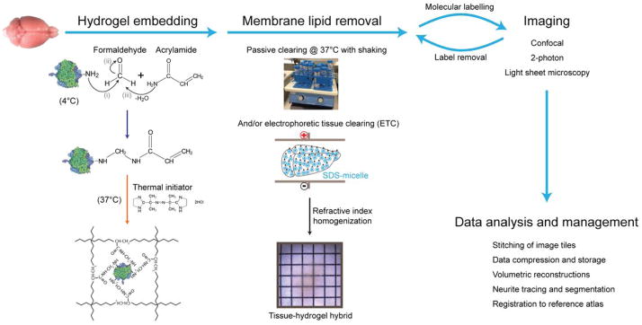
The tissue sample, e.g. an intact mouse brain, is perfused with cold hydrogel monomer solution that contains a cocktail of acrylamide, bisacrylamide, formaldehyde and thermal initiator. Formaldehyde mediates crosslinking of biomolecules to acrylamide monomers via amine groups; presumptive chemistry of this process is shown. Hydrogel polymerization is initiated by incubating the perfused tissue at 37°C, resulting in a meshwork of fibers that preserves biomolecules and structural integrity of the tissue. Lipid membranes are removed by passive thermal clearing in SBC solution at 37°C or by electrophoretic tissue clearing (ETC). The resulting intact tissue-hydrogel hybrid can undergo multiple rounds of molecular and structural interrogation using immunohistochemistry and light microscopy. A dedicated computational infrastructure is needed to analyze and store the data. All animal experiments were carried out with Stanford University Institutional review panel approval.

Figure 2. Electrophoretic tissue clearing.

(a) Schematic of a multiplexed electrophoretic tissue clearing setup. (b) Implementation of two differently-sized ETC chambers fitting one brain (left) or up to four brains (right). Top pair of images: the two chambers are constructed similarly with regard to power and fluid inlet/outlet. Second image at left: internal arrangement of electrodes. Third image at left: dimension of electrode geometry: note centimeter-ruler for scale. Fourth image at left: positioning of a brain in the single-brain chamber. Second image at right: positioning of 4 brains in the multi-brain chamber. Third image at right: closeup of non-metallic mesh for brain positioning: similar composition and positioning for both chambers.

An additional feature of the stable hydrogel-tissue hybrid is that it can be subjected to multiple rounds of molecular interrogation. Typically, immunohistochemistry methods only allow investigation of 2–3 biomarkers at once in a tissue sample, but more simultaneous labels are required to define cells in terms of precise molecular/genetic identity, wiring, and activity history. This limitation is traditionally approached by combining information from multiple samples into a standard reference atlas. However, this strategy fails to fully phenotype individual cells, cannot capture the joint statistics among the different kinds of labels within a single preparation, and suffers from 3D alignment artifacts and variability among different individual tissue samples. By allowing multiple rounds of histochemical labeling and elution in the same tissue, CLARITY provides unusually rich access to molecular and structural information.

Imaging large clarified tissue volumes

The next major challenge after achieving access to clarified large tissues is to develop optimized and high-resolution deep imaging approaches. One of the most important components of any light microscopy system is the detection objective (Figure 3a), which sets the resolution that can be achieved and the maximum sample size that can be imaged. In this context, three critical parameters of a detection objective are: (a) working distance (WD), (b) numerical aperture (NA), and (c) optical aberration (color) correction, for multiple light wavelengths and immersion-medium refractive indices (Figure 3a). WD is the distance between the focal plane (or the imaging plane) and the physical edge of the objective lens, and therefore determines how deep one can image without physically touching the sample. NA describes how much of the emitted fluorescence signal can be collected by the objective and the diffraction-limited resolution that can be achieved (higher NA translates to improved resolution in wavelength-dependent fashion, according to the relationship defined by the Abbe diffraction limit of λ/2NA; Figure 2a). And the level of aberration correction defines, among other aspects, how well the acquired multi-color images are co-registered. There are trade-offs among these three parameters, and for imaging large clarified samples the investigator must strike a scientific question-guided balance constrained by the nature of the specific experimental system. Finally, the selected properties must be integrated in a microscope objective matched to the refractive index range of the immersion liquid and tissue sample, a property of fundamental importance¹⁵; we have accordingly advised objective manufacturers to facilitate development for CLARITY samples, and these new objectives are becoming available.

Figure 3. Imaging clarified samples.

(a) Key microscope objective parameters relevant to CLARITY are working distance (WD), numerical aperture (NA), refractive index (n), and multi-color correction. Working distance is the distance between the objective lens and the focal plane. Numerical aperture (NA) relates to the fraction of total emitted signal collected by an objective, and higher NA enables higher resolution. The graphs plot diffraction-limited lateral and axial resolution parameters as a function of NA, assuming λ=500 nm. (b) Comparison of confocal, two-photon and light sheet microscopy. Confocal achieves optical sectioning by employing a pinhole in front of the photomultiplier tubes (PMTs). Two-photon utilizes the fact that only simultaneous absorption of two photons (of longer wavelengths) results in fluorescence signal emission, an event more likely to occur at the point of highest light intensity in the sample i.e. the focal plane. Light sheet fluorescence microscopy achieves optical sectioning by selectively confining the illumination to the plane of interest. Confocal and two-photon are point scanning and hence inherently slow, whereas light sheet microscopy uses fast sCMOS/CCD cameras to image the selectively illuminated focal plane, resulting in 2 to 3 orders of magnitude faster imaging speed and minimal photo-bleaching.

In addition to optimized detection optics, the nature of the microscopy system is important for achieving high imaging speed and minimizing photo-bleaching. While confocal and two-photon microscopes have been the workhorse systems in volumetric imaging for the reasons described above, over the past two decades light sheet fluorescence microscopy has emerged as a powerful approach for high-speed volumetric imaging. Figure 3b compares the mechanistic foundations of these three imaging modalities. Confocal and two-photon are point-scanning techniques, detecting optical signals point-by-point to construct an image. Confocal achieves optical sectioning by the use of a pinhole at the detection focal plane to reject out-of-focus light, whereas two-photon utilizes the fact that only simultaneous absorption of two photons results in fluorescence emission, an event much more likely to occur at the point of highest light intensity in the sample (the focal plane). Light sheet microscopy, in contrast, builds upon a hundred-year-old idea to illuminate the sample from the side with a thin sheet of light, and detect the emitted fluorescence signal with an in-focus orthogonally arranged objective^16,17. The optical sectioning is achieved by the confinement of illumination to a selective plane, which allows use of fast CCD or sCMOS cameras to capture the whole image simultaneously, and results in an increase of 2–3 orders of magnitude in imaging speed compared to confocal and two-photon microscopy. Moreover, light sheet microscopy minimizes photo-bleaching (Figure 3b) by confining illumination to the plane of interest. Taken together, these properties of light sheet microscopy may be well-suited for the imaging of large clarified samples, consistent with previously-demonstrated utility for minimizing unnecessary illumination in living cells¹⁵, embryos^18–20, and large conventional histology samples^8,21.

Overview of procedure

We describe here advanced protocols for CLARITY. Prior to starting the CLARITY process reagents are prepared (step 1) and animals anaesthetized (step 2). The entire CLARITY process is termed clarification and includes hydrogel monomer infusion and crosslinking (steps 3–8), thermally-triggered hydrogel polymerization (steps 9–11), passive or active lipid clearing (steps 12–14), and RI homogenization (step 20). If required, samples are immunostained (steps 15–19) prior to the RI homogenization. The clarified samples are then deep imaged using optimized objectives, adapted confocal methodologies, and CLARITY optimized light-sheet microscopy (COLM) (Figure 4). The entire depth of the mouse brain (>5 mm) can be imaged at high resolution using CLARITY-optimized objectives (Figure 5,6,7,8b; Supplementary Video 1,2,3), and for high-speed collection of large clarified volumes, light sheet methods are 100–1000 times faster, leading to vastly decreased photo-bleaching (Figure 5,6; Supplementary Video 1, 2). We show here the first application of the new generation of CLARITY-optimized objectives now available from the major commercial sources including Leica and Olympus.

Figure 4. CLARITY optimized light-sheet microscopy (COLM) for large intact samples.

(a) Optical layout of the CLARITY optimized light-sheet microscope. Two light sheets are created from opposite sides; shown are galvanometer scanners, scan lens, tube lens and illumination objectives. The emitted fluorescence is imaged with an in-focus detection objective, tube lens and sCMOS camera. Illumination and emission filter wheels (motorized) are used to generate well-defined excitation light and emission signal bands respectively. The innovations required for COLM are discussed in b–d, and schematic shown in Supplemental Figure 2. (b) Optically homogeneous sample mounting framework for large intact samples. Clarified samples, such as intact adult mouse brain, are mounted in a quartz cuvette filled with refractive index matching solution such as FocusClear. Note that the refractive index of quartz glass (~1.458) is nearly identical to that of FocusClear (~1.454). A bottom-adapter is used to attach the cuvette to the xyz-theta stage in the sample chamber, which is then filled with a matching refractive index liquid (~1.454). This results in an optically homogenous sample manipulation system with minimal refractive-index transition boundaries. (c) Synchronized illumination and detection is achieved by synchronizing the scanning beam with the uni-directional readout of a sCMOS camera chip, resulting a virtual-slit effect that allows substantially improved imaging quality, as illustrated by the images shown acquired from the same plane with COLM and with conventional light-sheet microscopy. The graph at right compares the signal intensity profile of a field acquired with COLM (red) and conventional light-sheet microscopy (blue). (d) Large clarified samples can have significant refractive index inhomogeneity, resulting in the need for correction of misalignment of illumination with the focal plane of the detection objective. We achieve this with a linear adaptive calibration procedure before starting the imaging experiment as described in Step 22B. All scale bars: 100 μm.

Figure 5. Ultrafast imaging of whole mouse brain using COLM.

(a) Volume rendering of whole mouse brain dataset acquired from an intact clarified Thy1-eYFP mouse brain using COLM. (b), (c) and (d) illustrate internal details of the intact mouse brain volume visualized by successive removal of occluding dorsal-side images. The brain was perfused with 0.5% acrylamide monomer solution, and clarified passively at 37°C with gentle shaking. Camera exposure time of 20 ms was used, and the refractive index liquid 1.454 was used as immersion media. The entire dataset was acquired in ~4 hours using a 10X, 0.6 NA objective. Video S1 demonstrates visualization of the dataset at high resolution.

Figure 6. Fast high-resolution imaging of clarified brain using COLM.

3.15 mm x 3.15 mm x 5.3 mm volume acquired from an intact clarified Thy1-eYFP mouse brain using COLM with 25x magnification; the brain had been perfused with 0.5% acrylamide monomer solution. The complete image dataset was acquired in ~1.5 hours; for optimal contrast the LUT of zoomed-in images was linearly adjusted between panels. (a) and (b) show magnified views from panel (c) region defined by yellow squares. (d)–(i) show maximum-intensity projections of over a 50 micron-thick volume, as shown by the progression of cyan and yellow boxes and arrows. Camera exposure time of 20 ms was used; refractive index liquid 1.454 was used as the immersion medium. High resolution details of the data set are provided in Video S2. All scale bars: 100 μm.

While resolution in any light microscope is limited by the laws of diffraction (λ/2NA = ~180 nm), the emergence of super-resolution (or “diffraction unlimited”) imaging methods, such as STED/RESOLFT and PALM/STORM (see recent review²²), could in the future allow a further 4–5 fold improvement in achievable resolution. As a final comment for future work, we note that very large datasets result from this new capability for high-speed imaging of large tissue volumes at high resolution, and extensive innovation will be needed in image analysis and data management (for example, if the intact 0.3cc mouse brain is represented by 0.5x0.5x0.5 cubic-micron 16-bit voxels, at least 4.8 terabytes of raw data result). Fortunately, big-data and high-performance computing have led to advanced image-compression technologies such as JPEG 2000 3D, increased computational capacity with GPU parallel computation technology, and cloud infrastructures (such as Amazon S3) for data storage and sharing. We expect that the integration and application of these methods to CLARITY will allow increasingly complete access to, and understanding of, the molecular and structural organization of large intact tissues.

MATERIALS

REAGENTS

Imaging samples here were prepared from adult Thy1-eYFP or WT mice.

CAUTION Experiments on animals must conform to National and Institutional regulations. Hydrogel monomer solution

• 40% Acrylamide solution (Bio-Rad, cat. no. 161-0140) ! CAUTION Acrylamide monomers are toxic. Perform all procedures in a fume hood.

• 2% Bis-Acrylamide solution (Bio-Rad, cat. no. 161-0142) ! CAUTION

• 16% Paraformaldehyde (Electron Microscopy Sciences, cat. no. 15710-S) ! CAUTION PFA is toxic. Perform all procedures in a fume hood.

• Polymerization Thermal Initiator VA044 (Wako, cat. no. VA-044)

• 10X PBS

Clearing Solution

• Boric Acid (Sigma, cat. no. B7901)

• Sodium Hydroxide pellets (EMD, cat. no. SX0590-3)

• SDS (Sigma cat no. L337 or Amresco cat no. 0837)

Refractive index matching and imaging solution

• FocusClear (CelExplorer Labs)

• MountClear (CelExplorer Labs)

• 87% Glycerol

• Custom Refractive Index liquids (RI 1.454, cat. no. 1806Y, Cargille Labs)

Immunostaining reagents

• 1XPBS with Triton-X (0.1%)

• Primary and Secondary Antibodies (see Table 1 for examples if antibodies we have used)

Table 1.

Antibodies for staining a 1mm-thick tissue block in 1ml PBST.

Volume (μL)	Antibody	Supplier
10–20	anti-TH	#ab113/Abcam, or affinity-purified anti-TH #ab51191/Abcam for lower background)
10–20	anti-PV	#ab32895 or #ab11427/Abcam
5–10	anti-GFAP	#ab53554/Abcam
5–20	anti-Synapsin-1	#ab64581/Abcam
10–20	anti-PSD-95	#ab2723 or #ab12093/Abcam
10–20	anti-MBP	#MBP/Aves
5–10	anti-somatostatin	#T-4103/Peninsula
5–10	anti-ChAT	#ab144p/Millipore
10–20	anti-GFP	Alexa-conjugated #A21311/Invitrogen, Alexa-conjugated #A31851/Invitrogen, #G10362/Invitrogen
20	anti-MAP2	ab32454/Abcam
10	anti-neurofilament	NFL/Aves, NFM/Aves, or NFH/Aves

EQUIPMENT

Hydrogel polymerization

• Vacuum pump (Buchi, cat. no. V-700)

• Desiccation chamber (any)

• Nitrogen supply (any)

Electrophoretic Tissue Clearing (ETC) chambers

• 60 mL Nalgene bottles for one-brain ETC chamber (Thermo Scientific, cat. no. 2118-0002)

• 125 mL Nalgene bottle for four-brain ETC chamber (Thermo Scientific, cat. no. 2118-0004)

• Push-to-connect fittings for constructing ETC chamber (McMaster-Carr, cat. no. 9087K14)

• Platinum wire 0.5 mm (Sigma Aldrich, cat. no. 267201-2G)

• Banana plug (Invitrogen, cat. no. EI9021)

• Sample holder (BD Falcon, cat. no. 352340)

• Mesh to fix sample orientation (McMaster-Carr, cat. no. 9275T38)

• Power supply (Bio-Rad, cat. no. 164E5052)

• Power supply adapter (Bio-Rad, cat. no. 164E5064)

• Water Circulator (Lauda Brinkmann, cat. no. RE 415)

• Tubings (McMaster-Carr)

• Filters (McMaster-Carr, cat. no. 4448K35)

• Adhesive (McMaster-Carr, cat. no. 746A17)

Sample mounting and Imaging if using a confocal microscope

• Wellco dish (Pelco(Ted-Pella), cat. no. 14032E120)

• BluTack Putty

• Kwik-Sil (World Precision Instruments, KWIKESIL)

• Microscope slides

• Cover slips

• Confocal microscope. The results shown here were obtained using an Olympus FV1200 microscope.

• CLARITY-optimized objectives (Now available from major commercial sources such as Leica or Olympus) Figure 7 and Supplementary Video 1 show results obtained using a 25X, 0.95 NA, 8 mm WD objective resulting in a 5 mm deep stack. Figure 8a,c shows results obtained using a water-immersion 10X, 0.6 NA, 3 mm.

Figure 7. Optimized confocal microscopy of clarified samples.

1.837 mm X 0.959 mm X 5 mm volume imaged from an intact cleared Thy1-eYFP mouse brain using a confocal microscope at 25X magnification. Brain was perfused with 4% acrylamide monomer solution. a: Rendering of entire volume. Images were acquired in top to bottom direction, corresponding to dorso-ventral brain axis. b, c, d and e are maximum-intensity Z-projections (1 mm, 1 mm, 1 mm, 1.7 mm thick respectively) at different imaging depths as marked by cyan arrow. f–i: Magnified images of the regions marked by yellow squares in b–e. Video S3 details 3D rendering of the entire volume. Scale bars: 100 μm.

Figure 8. Molecular interrogation of clarified tissue.

(a) Parvalbumin (PV) positive neurons in a 1 mm thick tissue block of mouse brain, labeled using anti-PV antibody. The brain was perfused with 4% acrylamide monomer solution. The tissue block was imaged using confocal microscopy. Images represent maximum intensity projections. (b) Whole brain immunostaining to label all PV positive neurons in an intact mouse brain. Panels show labeled cells at different depths in the sample. The brain was perfused with 4% acrylamide monomer solution and clarified passively. The intact brain was imaged using COLM with a 25x objective. (c) Multiple rounds of immunostaining in the same tissue block (1% acrylamide monomer solution). Left-to-right: first round of immunostaining for PV, followed by label elution via overnight (~12 hours) incubation in clearing buffer at 60°C, in turn followed by a second round of immunostaining for PV. DAPI present in the first round was successfully eluted as well (not shown). All images represent maximum Z-projections and all scale bars are 100 μm.

REAGENT SETUP

Hydrogel monomer (HM) solution

Prepare 400 ml HM solution by mixing 40 mL of 40% acrylamide (4% final concentration), 10 mL of 2% bisacrylamide (0.05% final concentration), 40 mL of 10X PBS, 100 mL of 16% PFA (4% final concentration), 210 mL of distilled water and 1g of VA-044 thermal initiator (0.25% w/v final concentration). Keep all the reagents on ice; aliquot 40 mL of the HM solution into 50 mL Falcon tubes and store at −20°C until needed (several weeks). Acrylamide and bisacrylamide concentration in HM solution can be proportionally reduced to speed up the clearing process. We have successfully employed concentrations of 0.5%/0.0125% acrylamide/bisacrylamide ranging up to 4.0%/0.05%; however we recommend lower acrylamide/bisacrylamide concentrations to start with as clearing speed is increased several-fold. Lower concentrations should increase the pore size of the hydrogel and hence also allow faster diffusion of antibodies, but at the potential cost of increased biomolecular content loss in the clearing process. Higher concentrations could provide better preservation for biomolecules, but lead to slower tissue clearing and immunohistochemistry time.

SDS/borate clearing buffer (SBC)

Prepare stocks of 20% SDS (in H₂O) and 1 M boric acid buffer (pH adjusted to 8.5). These stocks can be stored at room temperature for several weeks. Final clearing buffer is freshly prepared by diluting 20% SDS and 1 M boric acid buffer 5-fold in distilled water.

EQUIPMENT SETUP

Electrophoretic Tissue Clearing (ETC) setup (optional)

A detailed schematic and photographs are shown in Figure 2. Construct ETC chambers by: (a) inserting two zig-zag shaped platinum wire electrodes, bound to banana plugs, at the bottom of the Nalgene bottles, and (b) inserting two push-to-connect fittings to provide the inlet for SBC buffer (in the Nalgene bottle body) and the outlet (in the center of the bottle lid). A soldering rod can be used to create appropriate holes by melting the plastic, and strong epoxy adhesives can be used to glue electrodes and inlet/outlet push-to-connect fittings. Two different sizes of Nalgene bottles can be used for making one- or four-sample clearing chambers.

Use appropriate tubing (eg, 1/2 and 3/8 inch outer diameter tubes) to connect the ETC chambers to a refrigerated circulator. A water filter should also be used to keep the buffer free of any particles. Tube fitting manifolds can be used to collect multiple ETC chambers to a single buffer circulator. Using 4 of the four-sample ETC chambers, up to 16 mouse brains can be cleared in less than a week with one circulator.

Regular monitoring of critical parameters such as buffer temperature, flow rate, pH and electric current flow levels, should be performed either manually or using automated real-time readouts. Figure 2 summarizes the entire ETC setup.

CLARITY optimized light-sheet microscopy (COLM)

A light sheet microscope consists of a standard wide field detection optical arm, which includes the detection objective, the tube lens and a camera, and the orthogonally-arranged independent illumination arm consisting of a low NA objective, tube lens and either a cylindrical lens to generate a static light sheet or galvanometer-scanners/f-theta lens for creating dynamic light sheets with a Gaussian or Bessel beams^{8,18,24–26,29}. Conventional light sheet microscopy suffers from image quality degradation due to out-of-focus scattered light; several methods have been developed to help reject out-of-focus light in light-sheet (at some cost in imaging speed, increased photo-bleaching and instrumentation complexity), such as structured illumination ^27,28.

We developed CLARITY optimized light-sheet microscopy (COLM) to maximize compatibility of clarified samples with light sheet microscopy, using CLARITY objectives (25X and 10X, Olympus), a fast sCMOS camera, two-axis galvo scanners along with the f-theta lens, a low NA objective to generate dynamic light sheets using a Gaussian beam, an optimized sample chamber (detailed in the following section) and an xyz-theta sample mount stage that provides a long travel range of 45 mm in each of the dimensions to allow imaging of large samples (Figure 4). The control electronics design and parts for COLM are summarized in Figure S2. COLM employs synchronized illumination-detection to improve imaging quality, especially at higher depths (Figure 4c), exploiting the uni-directional readout (as opposed to standard bi-directional; though at cost of imaging speed) mode available in the next generation sCMOS cameras. The scanning beam (which creates the dynamic light sheet) is synchronized with the uni-directional single line readout of the emitted signal, resulting in a virtual confocal-slit arrangement, which rejects out-of-focal-plane signal due to scattering deeper in the sample. Automated-alignment parameter calibration (using linear adaptation) in COLM corrects for misalignment artifacts across the whole sample space (Figure 4d); corresponding control software is available on request.

Sample mounting apparatus for COLM

The final component of COLM is a CLARITY-optimized sample mounting strategy that minimizes optical inhomogeneity along the detection path (Figure 4b). Clarified whole mouse brain (or any large clarified intact tissue such as a spinal cord) is mounted in a cuvette made of fused quartz glass (standard cuvettes used for spectrophotometer measurements) filled with FocusClear; note that the refractive index of fused quartz (~1.458) is nearly identical to that of FocusClear. Using a bottom-adapter (Figure 4b), the sample cuvette is mounted onto the xyz-theta stage, inside the sample chamber (Figure 4b). The much larger chamber is then filled with a relatively economically-priced custom refractive index matching liquid (RI 1.454, cat. no. 1806Y, Cargille Labs), resulting in an optically homogeneous sample manipulation system. RI liquid costs several hundred dollars per half liter, which is enough to fill the sample chamber (and more than an order of magnitude cheaper than FocusClear) and can be re-used many times. The chamber also can be filled with 87% glycerol, which is workable but is highly viscous and more likely to cause and maintain inhomogeneities such as gradients and bubbles in large volumes.

Computational workstation for data analysis

Since the image data sizes are expected to be very large, it is important to employ a computational workstation with abundant RAM, multi-core CPUs and an excellent graphics card. Data shown here were handled on a workstation with the following configuration: Intel server board S2600CO, two Intel Xeon E5-2687W 8C CPUs, ~130 GB of DIMM RAM, ~8 TB of hard disk (Seagate Savvio 10K), NVidia K5000 graphics card and a high-resolution monitor (NEC MultiSync PA301W 30 inch 2560x1600).

PROCEDURE

Transcardial perfusion of mouse brain with hydrogel monomer solution

• 1|Prepare the hydrogel monomer stock solution by thawing frozen vials on ice or in refrigerator. Gently mix the thawed monomer solution by inverting. Keep all reagents on ice during whole procedure.

  CRITICAL STEP Make sure there is no precipitation floating in the monomer solution; this is an indicator of spontaneous polymerization of stored monomer solution.

• 2|Anaesthetize animals by injecting Beuthanasia-D (100 mg/kg of body mass). Follow appropriate institutional guidelines for handling animals.
• 3|Perfuse 20 mL of ice cold 1X PBS at approximately 10 mL/min. Make sure that the PBS becomes colorless by the end of perfusion. If not, repeat the washing step with 20 mL more PBS.
• 4|Perfuse the animal with hydrogel monomer solution at about 10 mL/min. Recover the brain (or other tissues) from the animal and place in the remaining 20 mL hydrogel monomer solution. Incubate at 4°C for a minimum of 1 day. Protect the sample from light if fluorophores are present. ! CAUTION PFA and acrylamide monomer are toxic. Perform all procedures in a fume hood.

  CRITICAL STEP Stiffening of muscles is indicative of successful perfusion.

  PAUSEPOINT Tissues can be kept at 4°C for up to 2 days.

Preparation for tissue embedding

CRITICAL Residual oxygen must be removed from the tissue sample. This section (steps 4–7) describes how to de-gas the falcon tube that contains the tissue sample using a standard vacuum pump and desiccation chamber, and nitrogen gas supply.

• 5|Place the 50 mL conical tube on a rack in the desiccation chamber. Partially open the cap to allow gas exchange.

  ! CAUTION. PFA and acrylamide monomer are toxic. Perform steps 5–8 in a fume hood.

• 6|Open the nitrogen tank main valve, and adjust the control valve to fill the desiccation chamber with nitrogen gas. Next, toggle the desiccation chamber valve from nitrogen gas in-flow to the vacuum pump outlet.
• 7|Turn on the vacuum pump. Verify that the chamber is under full vacuum by testing the chamber lid. Keep it running for 10 minutes.
• 8|Switch the vacuum pump off and slowly the nitrogen will fill the chamber. Carefully open the chamber just enough to reach the tubes and tighten the lids while continuously purging with nitrogen gas.

  CRITICAL STEP Oxygen inhibits hydrogel polymerization. Therefore, make sure to remove as much residual oxygen as possible.

Tissue embedding by hydrogel polymerization

• 9|Transfer the air-tight closed falcon tube to 37°C room or a water bath for 3–4 hours. Gentle shaking helps in heat transfer for achieving robust and uniform polymerization.

  CRITICAL STEP Make sure that the hydrogel has fully solidified before proceeding to the next step. If not the repeat the de-gassing section (steps 5–8) and transfer to 37°C again. Note that lower acrylamide concentration (such as 0.5%) hydrogels do not solidify fully upon polymerization. Therefore, the de-gassing step is especially critical.

• 10|Carefully extract the brain (or other tissues) from solidified hydrogel by softly rubbing all the hydrogel from the surface. Kimwipes can be used to remove the residual gel from the tissue surface. ! CAUTION Hydrogel waste disposal should be conducted according to local regulations for hydrogel monomers and cross-linkers (e.g. acrylamide and PFA).
• 11|Wash the tissue sample twice with 50mL of SBC buffer for 24 hours at room temperature (25°C) to dialyze remaining PFA, initiator, and monomer. The brain sample can be left in SBC buffer at 37°C until ready for clearing. If desired, the tissue sample can be cut into ~1–2mm blocks immediately after embedding for accelerated clearing and staining as described below.

Tissue clearing by passive thermal diffusion or by electrophoretic tissue clearing (ETC)

CRITICAL For successful completion of lipid removal, it is important to tune the clearing parameters to tissue properties and dimensions. With ETC, tissue orientation relative to the electric field is important; to minimize distance traveled by SDS micelles and maximize SDS flux, tissue blocks or organs should be oriented with the shortest axis parallel to the electric field direction. Whenever allowed by speed, tissue properties, and other constraints, we advise passive thermal clearing rather than ETC.

• 12|Start clearing tissue passively (option A) or using ETC (option B). (ETC is faster but can damage tissue and reduce immunostaining efficacy).

  Option A) Passive clearing of hydrogel-embedded tissue (passive CLARITY)

  • Gently shake the sample at 37°C. Higher temperatures up to 60°C can be used for faster clearing but this may quench endogenous fluorescence in cases where that is a relevant consideration. The passive clearing process also can be sped up while retaining its key advantages by using lower concentrations of acrylamide/bisacrylamide in the HM solution as discussed in REAGENT SETUP.

  Option B) Electrophoretic tissue clearing (ETC) of hydrogel-embedded tissue

  1. Transfer the sample to an ETC chamber as shown in Figure 2. Use mesh sheets for fixing the orientation of tissue relative to the electric field direction, and close the chamber as shown in Figure 2. Up to four brain samples can be cleared in one ETC chamber, and up to 16 in one multiplexed setup (Figure 2).

  2. Turn ON the clearing solution refrigerated circulator first, and then switch ON the power supply. Different combinations of voltage and buffer temperature can be used for the ETC process. For adult mouse brain samples, we recommend running the ETC process at 25V and 37°C for about 3–5 days, with regular checks on pH of the clearing buffer; immediately change the buffer if the pH drops below 7.5.

  CRITICAL STEP Power input into the ETC chamber results in heat generation in the solution, which needs to be dissipated by the circulating clearing solution. In general, higher temperature and higher voltage results in faster clearing of the tissue, but may lead to a higher risk of sample, epitope, or fluorescence loss (see also ref. 23 for detailed characterization of the effect of temperature on SDS micelle sizes).

• 13|Check for completion of tissue clearing by assessing for transparency (easy visualization of high-contrast signals such as a black-and-white grid or printed text through the tissue) and homogeneity (even distribution of transparency across the tissue; Figure S1). Once tissue is clearer, proceed to next step.
• 14|Wash twice in PBST or boric acid buffer (1M/pH8.5 with 0.1%Triton X-100) for 1 day at 37°C. For whole-brain CLARITY, we recommend not only low-percentage (1%) acrylamide monomer and thorough passive clearing in SDS, but also a wash in boric acid buffer/0.1%Triton X-100 (instead of PBST) to remove the remaining SDS. If proceeding to immunostaining, (which should typically be conducted in PBST), transfer the brain from boric acid/0.1%Triton X-100 to PBST 30 min prior to incubation with primary antibody (step 16, below).

Molecular labeling

CRITICAL A tissue sample may have endogenous transgenic expression of fluorophores to label molecular and structural details in the sample, but additionally, immunohistochemistry can be used for labeling structure and molecules of interest. Follow this section for immunostaining a thick tissue block or intact mouse brain. If you do not wish to perform immunohistochemistry proceed direct to step 21.

• 15|Ensure the tissue has been washed thoroughly in PBST (or boric acid buffer/0.1%Triton X-100 wash for whole brains) for at least 1 day at 37°C.
• 16|Incubate in primary antibody/PBST solution (beginning with 1:50 dilution) for 2 days at 37°C for tissue blocks, or for up to a week for the whole intact brain. Note that ~1M borate/0.1%Triton X-100 buffer (pH 8.5), in some cases, can also be used in place of PBST for antibody incubations to reduce background staining. As with any staining procedure, it is important to systematically optimize staining conditions (detergent, temperature, concentrations, and so on) for the particular antibody used. Table 1 lists examples of antibodies we have used to incubate a 1 mm-thick block in 1 mL solution¹³: A whole mouse brain can be incubated in 5 mL solution with scaled-up antibody volumes supplemented periodically; for example, 50 μL antiTH Ab as above can be added, followed by 20 μL more every two days for ~ 1week.

  CRITICAL STEP High antibody concentrations (1:20–1:100) are usually required for effective immunostaining to ensure deep penetration into tissue and to overcome the large aggregate number of antibody binding sites over the volume. 1:1000 dilutions typically lead to inadequate tissue penetration. A second major factor for successful immunostaining is complete removal of lipids during clearing.

  CAUTION Make sure there is no microbial growth during long incubations at 37°C; 0.01% w/v sodium azide can be added to the primary and secondary antibody solutions.

• 17|Wash off the primary antibodies with PBST buffer at 37°C for 1 day for tissue blocks and for 2–3 days for whole brain (refresh buffer every 4–6 hours).
• 18|Incubate with desired secondary antibody (1:50–1:100) in PBST for 2 days at 37°C for tissue blocks or for up to 1 week for whole brain. Note that a nuclear labeling dye, such as DAPI, can also be added at this step.
• 19|Wash off the secondary antibodies with PBST at 37°C for 1 day for tissue blocks and 2–3 days for whole brain.

  PAUSEPOINT The sample can be stored in PBST (with 0.01% sodium azide) at 4°C for up to a week.

• 20|To prepare for imaging, transfer the tissue into FocusClear for refractive index homogenization as described below. Note that it is possible to elute (remove) prior labels by incubating in clearing buffer at 60°C overnight (Figure 9c) in preparation for another round of labeling after imaging has been performed. Once labels have been removed repeat steps 15–19 with alternative antibodies.

Refractive Index homogenization

CRITICAL Due to inherent refractive index inhomogeneity of tissues, photons (both the excitation light as well as the emitted fluorescence signal) scatter when traveling through the sample, limiting the quality of images that can be acquired as well as the imaging depth that can be achieved. Therefore, a crucial final part of sample preparation is the homogenization of the microscopic environment inside the tissue using a chemical solution that matches closely the average refractive index of the tissue. FocusClear (CelExplorer Labs) and 87% glycerol have been extensively tested¹³ for this purpose; both complete the tissue transparency process but currently best results are achieved with FocusClear.

• 21|Transfer the PBST-washed tissue into FocusClear (or 87% glycerol) and periodically check visual clarity of the sample over the next few hours. 1 or 2 mm thick tissue blocks will typically complete the RI homogenization process in about 1 hour whereas an intact mouse brain can take several hours. Treatment at 37°C accelerates this process several-fold. Once the tissue has been fully clarified, immediately proceed with imaging preparations (described below) or return tissue to PBST.

  PAUSEPOINT Prior to RI homogenization (or after), tissue may be stored indefinitely in PBST (with 0.01% sodium azide) at 4°C, but extended incubation of tissue in FocusClear is not advised since this can result in formation of a white opaque precipitation that will hinder deep imaging.

Imaging and analysis

• 22|CLARITY allows access to deep tissues using multiple light microscopy modalities; we describe here protocols for deep imaging of clarified tissues using advanced confocal (option A) and light sheet microscopies (option B) (Figures 3–8). Since confocal microscopes are widely available, we include an optimized procedure to image through the entire depth of a clarified intact mouse brain with confocal methods. Most of these principles will apply similarly to the other imaging modalities; indeed we also discuss the high-speed, high-resolution light sheet microscopy of clarified samples, and present datasets to demonstrate compatibility.

  1. Confocal imaging

     1. Sample Mounting. Mount a whole clarified mouse brain between two Wellco dishes as follows. First place a Wellco dish upside down, with the glass surface facing up. Prepare 7–10 mm thick diameter uniform cylindrical tube of BluTack putty clay by smoothly rubbing between gloved hands. Use the putty tube to create a well on the glass surface by folding it in a circle, leaving a small opening on joining ends. Place the clarified brain carefully inside this well, preferably with the dorsal surface up.

     2. Place another Wellco dish on top of the well such that the glass side directly interfaces with the putty walls. Gently press on the top Wellco dish till the glass touches the brain surface, while keeping the two glass surfaces parallel. Make sure that the putty sticks well to the glass surfaces to avoid any leakages afterwards.

     3. Use the small joint opening in the putty wall to fill it up with FocusClear using a 1000 ul pipette. Seal this hole by using Kwik-Sil silicone adhesive, and leave it to dry for about 30 minutes, after which the sample is ready for imaging. CRITICAL STEP An important advantage of this sample mounting procedure is that it allows imaging from either side. Thick brain blocks can be mounted similarly using thinner putty walls, and even thinner slices (<2 mm) can be mounted using a standard glass slide and cover slip with a thin well of putty.

     4. Select appropriate objective. Numerical Aperture (NA) of the detection objective determines the maximum resolution that can be achieved. Figure 3a shows plots of diffraction-limited lateral and axial resolutions as a function of NA. For NA of 0.9, the optics can at best achieve ~0.278 microns lateral resolution and ~1.235 microns axial resolution (along the Z axis). The Nyquist sampling criterion suggests that the detected pixel size of the microscope should at least be 2-fold smaller than the resolution of the optics. Thus, for a 25X objective, optimal imaging will be achieved by adjusting pixel sampling (controlled by changing the number of pixels collected) such that the pixel size is 0.278/2 = 0.139 microns, and the z-spacing is 1.235/2 = ~0.617 microns. These settings will take full advantage of the objective capability, but the high pixel sampling density will slow imaging speed considerably. This tradeoff between image quality and imaging speed should be assessed for each system based on the constraints of the biological question.

     5. Determine the desired laser intensity. This is another critical parameter. High laser power will photo-bleach the sample quickly; therefore especially for large tissue volumes, power should be minimized. While this may reduce the signal level, signal can also be improved without increasing laser intensity by increasing the electronic gain, though higher gain may result in higher noise. Increasing pixel dwell time will also increase signal, but at the cost of increased imaging time and photobleaching.

     6. Select and add an appropriate immersion liquid between the glass dish and the microscope objective. The immersion liquid should ideally match the specifications of the microscope objective. For example, when using a water immersion objective, only water should be present between the glass and the objectives. However, if the refractive index of the immersion liquid is much different from that of the mounting liquid (such as FocusClear), optical aberrations may result, which become significant for deep imaging with high NA objectives. As a rule, the closer the refractive indices match, the better the image quality. Therefore, we show here the use of a custom CLARITY corrected objective for high-resolution deep imaging at 25X (Figure 7) in an optimized custom immersion oil with refractive index of 1.454 (cat. no. 1806Y, Cargille Labs), matching the refractive index of FocusClear. We also describe use of a water immersion 10X objective for high image quality in a clarified and immunostained tissue block (Figure 8a,c).

     7. Commence confocal imaging. Since the field-of-view of a microscope objective is often smaller than the sample itself, it may be necessary to collect multiple stacks in tiling arrangements, which are then stitched together to yield a large image volume. Many microscope objectives suffer from vignetting (in which image quality is lower at the edges than the middle). This artifact in the stitched images can be avoided by using a digital zoom of about 1.2 during imaging.

  2. CLARITY optimized light-sheet microscopy (COLM)

     1. Mount the sample (e.g. intact mouse brain), in a quartz cuvette of appropriate dimension, so that the sample remains stationary while imaging (Figure 4b). Note that many different sizes of quartz cuvettes are available from vendors (such as Starna Cells); however, in case the sample does not fit easily, a small piece of acrylamide gel (or similar transparent material) can be used to provide structural padding on the side opposite to the imaging side. For adult mouse brain, we recommend either 10 x 5 mm or 10 x 10 mm base cuvettes with padding, depending on age; these are standard sizes, but custom sizes can also be purchased from many vendors.

     2. Fill the cuvette with FocusClear, just enough to cover the entire sample. Using an adapter, the cuvette is mounted on the xyz-theta stage (Figure 4b). CRITICAL STEP. Avoid bubbles or dust particles as they will interfere with the imaging.

     3. Set tiling parameters. Some samples can be larger than the field of view of the objective used, and therefore will require tiling of image stacks to cover the entire sample. To specify the number of tiles, begin by defining the coordinates of the two opposite corners of the region of interest; we recommend 20% or more tile overlap. As with confocal imaging, specify the start and end z-position of the stack by finding the first and last image frames containing useful signal from the sample, and then set the desired z-step value.

     4. Adjust for any misalignment of the light sheet and the detection focal plane, which (particularly during imaging of large samples) can result in blurred images. Therefore, the light sheet and focal-plane alignment parameters need to be optimized over the entire sample space as defined in step iii. We achieve this by optimizing these parameters at every millimeter of tissue for all the tiles, and then linearly interpolating the values for z-steps in between these millimeter steps. Optimal parameters are identified by finding maxima in a specified neighborhood corresponding to the image quality measure; to automate this process, we implement an optical focus-quality measure, as the ratio of high frequency and low frequency signal in Fourier space.

     5. Initiate the imaging experiment and data collection.

3D reconstruction and analysis

• 23|Perform three-dimensional reconstructions either with commercial software (eg, Imaris from Bitplane or Amira) or via free/open-source projects (eg, Vaa3D, www.vaa3d.org). Typically, commercial software tools can be easier to use, though can be quite costly compared with open-source versions. The stitching of tiles of image stacks can either be performed using the microscope control software or open-source modules (eg, the stitching plugin in Fiji³², XuvTools³⁰, Vaa3D plugin^31,32 or TeraStitcher³³). For the sample results shown here, the stitching of tiles was performed with TeraStitcher (for lightsheet) or the Fiji stitcher plugin (for confocal). Similarly, manual or semi-automatic tracing of neuronal morphology can be performed using with specific modules in commercial software such as Imaris and Amira, or with open-source tools such as Neuromantic³⁴.

TIMING

• Steps 1–4, Infusion of hydrogel monomer solution: 1 d

• Steps 5–11, Hydrogel polymerization and tissue washing: 1d

• Steps 12–14, Tissue clearing: 5 d (ETC) to 3 weeks (passive thermal clearing) for 1% acrylamide HM solution-embedded whole adult mouse brain)

• Step 15–20, Immunostaining, single-round:

  • 1–2 mm tissue block: 2–3 d with a labeled primary antibody or 5–6 d for conventional 2-step primary/secondary antibody stain

  • Whole mouse brain: 7–10 d with a labeled primary antibody or 2–3 wks for conventional 2-step primary/secondary antibody stain

• Step 21, Refractive index homogenization: 4–5 h

• Steps 22, Imaging: 3 h-3 d

• Step 23, stitching and 3D reconstruction: 1h - 1d

TROUBLESHOOTING

See Table 2 for troubleshooting guidance.

Table 2.

Troubleshooting

Step	Problem	Possible reason	Possible solution
Hydrogel embedding related, steps 1–11	Trans-cardiac perfusion is not possible (for example, human tissue samples)		Passively infuse the monomers into post-fixed tissue by incubating the sample in hydrogel monomer solution at 4°C for several days (depending on the tissue size) with gentle shaking. For example, 3–4 days of passive infusion is sufficient for a pre-fixed mouse brain.
	Hydrogel polymerizes	Hydrogel can polymerize at room temperature	Keep the tubing and needles on ice during perfusion to prevent clogging. It is also critical to use ice-cold PBS to chill the tissues before perfusing with hydrogel monomer solution.
ETC clearing related (steps 12–14)	Poor tissue clearing.	The two electrodes may be placed too far away from each other	Keep as close as possible, without touching the sample. This is critical to create the highest current density to drive tissue clearing.
		Over-polymerization of hydrogel	Do not leave the sample in monomer solution (at 37°C) for more than 5–6 hours. If the samples are polymerized overnight, this will make tissue clearing and staining very difficult.
		Clearing buffer needs to be refreshed.	The SBC buffer needs to be refreshed once the pH goes below 7.5, otherwise clearing efficiency will drop. Using increased voltage or larger electrodes will increase the rate of buffer consumption; therefore the buffer may need to be changed more frequently under these conditions.
	Tissue damage during clearing: Black deposits on samples and electrodes.	Black deposits will form on the cathode over time (on the order of several days), and will gradually start to transfer to the tissue surface, if left unattended.	The electrodes can be easily cleaned by reversing the voltage polarity, and running the power and buffer flow for 10–20 minutes. Regular cleaning of electrodes (every 3–4 days) will prevent black deposits on the samples.
	Tissue damage during clearing: Sample burnt or turned yellow.	High temperature (resulting from higher current and/or insufficient heat dissipation due to low flow rate) will cause yellowness or even burn or melt the samples.	It is critical for individual users to determine the optimal combination of voltage, temperature and flow rate settings based on the sample properties and chamber design.
	Loss of fluorescence.	High temperature/voltage can quench fluorescence, as can high acidity.	It is critical to maintain the temperature at 37°C and pH above 7.5.
	White precipitate formation after FocusClear treatment.	An opaque white deposit may form inside samples left in FocusClear for more than 1–2 days.	Any residual SDS from the clearing solution significantly accelerates this deposition. It is very important to completely remove residual SDS by thoroughly washing the samples with PBST (0.1–0.2% TritonX100) several times over 1–2 days (refresh PBST at least every day). In general, samples should never be stored in FocusClear, but returned to PBST at 4°C, as soon as imaging is completed
Staining and imaging related (steps 15–22)	Low staining reagent/label penetration	Tissue sample is not very well cleared in terms of lipid removal.	Clearing can be further improved by passively clearing the samples in SBC solution (at 37°C with gentle shaking) for additional days after ETC. Note that whenever feasible, perform passive thermal clearing for tissue destined for subsequent immunostaining.
		Poor antibody penetration	Up to 1% TritonX-100 (more typically 0.2–0.5%) in PBS can be employed to facilitate further antibody penetration.
		Insufficient incubating solution.	Use large volumes of incubating solutions for big tissue samples. Frequent refreshment of the buffer and antibody can lead to further improvement.
	Heavy background or weak signal	Samples that become damaged during ETC tend to have high auto-fluorescence background.	Refer to the previous section for preventing sample damage. Note also that ETC is not always necessary for small tissue samples, and prolonged passive clearing can be a very suitable option in many cases.
		Long incubation in FocusClear can lead to fine precipitation (invisible to the naked eye) that generates heavy auto-fluorescence.	FocusClear treatment should be kept to the minimum needed, and residual SDS must be removed from the samples.
		Photobleaching	To prevent photobleaching, minimize any unnecessary light exposure to the sample before and during imaging. Keep laser power to a minimum while setting up the imaging parameters for the tissue.

ANTICIPATED RESULTS

Figure 4b compares the images taken using standard light sheet or CLARITY optimized light sheet microcopy (COLM). We performed imaging of whole-brain samples using 10X or 25X magnification objectives (Figures 5,6; Supplementary Videos 1,2). Multiple factors contribute to image quality at this whole brain level; for example, independent of imaging modality, the sample needs to be clarified extremely well with minimum tissue damage, and the detection optics including objective must be well-corrected for expected optical aberrations, even with confocal or two-photon methods.

CLARITY allows molecular and structural interrogation of tissue by allowing deep imaging of transgenic and/or biochemically labeled tissue samples. As discussed above, to achieve the best imaging quality, careful preparation of the sample and the optical setup is crucial. First, as demonstrated in Figure 3, key relevant properties of the objective must be considered including numerical aperture, working distance, color correction, and refractive index correction. Several commercial objectives are available that possess high NA (>1.0) and color correction at multiple wavelengths, but at the cost of working distance; conversely longer working distance objectives are available at the cost of numerical aperture. We explored the emerging commercially available and custom solutions, and found that it is indeed possible to achieve deep high-resolution and overall high-quality imaging in clarified samples (Figures 5–8; Supplementary Videos 1–3). For example, Figure 7 presents a 5 mm deep brain volume, spanning the dorsal to the ventral surface of the mouse brain, acquired using a confocal microscope and a CLARITY optimized 25X, 0.95 NA objective (Olympus). Other water immersion, oil immersion, or air objectives may also prove to be useful for quality imaging deep in tissue.

The major limitations of confocal and two-photon microscopes are 1) slow speed owing to point scanning mechanisms (Figure 3) and 2) damage to tissues and fluorophores due to redundant illumination of the whole sample for every optical plane imaged, limiting the size of sample that can be imaged in a reasonable timeframe before the sample is completely photobleached (particularly in the case of confocal microscopy). While not as severe as with confocal, it is well-documented (and particularly relevant here for long imaging times) that two-photon microscopy also leads to photo-bleaching and other non-linear tissue damage^35–37. Light sheet microscopy now emerges as an alternative for fast 3-dimensional imaging of large clarified samples, as described above.

We assessed the compatibility of clarified samples with light sheet, observing greater than 2 orders of magnitude faster imaging speed with minimal photobleaching; for example, it was possible to image an entire mouse brain in about 4 hours using a 10X magnification objective and in about 1.5 days using a 25X objective, as opposed to many days and months, respectively, with a confocal microscope. CLARITY optimized light-sheet microscopy (COLM) is especially well suited for interrogation of large tissue samples labeled with transgenic or histochemical approaches. The increased speed of acquisition and higher quality of data generated via CLARITY using new microscopy methods, combined with high-speed CLARITY processing itself enabled by parallelized and efficient tissue transformation protocols described here, together define a versatile and efficient platform for structural and molecular interrogation of large and fully assembled tissues.

References

- 1.Bock DD, et al. Network anatomy and in vivo physiology of visual cortical neurons. Nature. 2011;471:177–182. doi: 10.1038/nature09802. [DOI] [PMC free article] [PubMed] [Google Scholar]
- 2.Briggman KL, Helmstaedter M, Denk W. Wiring specificity in the direction-selectivity circuit of the retina. Nature. 2011;471:183–188. doi: 10.1038/nature09818. [DOI] [PubMed] [Google Scholar]
- 3.Conchello JA, Lichtman JW. Optical sectioning microscopy. Nature methods. 2005;2:920–931. doi: 10.1038/nmeth815. [DOI] [PubMed] [Google Scholar]
- 4.Helmchen F, Denk W. Deep tissue two-photon microscopy. Nature methods. 2005;2:932–940. doi: 10.1038/nmeth818. [DOI] [PubMed] [Google Scholar]
- 5.Tang J, Germain RN, Cui M. Superpenetration optical microscopy by iterative multiphoton adaptive compensation technique. Proceedings of the National Academy of Sciences of the United States of America. 2012;109:8434–8439. doi: 10.1073/pnas.1119590109. [DOI] [PMC free article] [PubMed] [Google Scholar]
- 6.Micheva KD, Busse B, Weiler NC, O’Rourke N, Smith SJ. Single-synapse analysis of a diverse synapse population: proteomic imaging methods and markers. Neuron. 2010;68:639–653. doi: 10.1016/j.neuron.2010.09.024. [DOI] [PMC free article] [PubMed] [Google Scholar]
- 7.Ragan T, et al. Serial two-photon tomography for automated ex vivo mouse brain imaging. Nature methods. 2012;9:255–258. doi: 10.1038/nmeth.1854. [DOI] [PMC free article] [PubMed] [Google Scholar]
- 8.Dodt HU, et al. Ultramicroscopy: three-dimensional visualization of neuronal networks in the whole mouse brain. Nature methods. 2007;4:331–336. doi: 10.1038/nmeth1036. [DOI] [PubMed] [Google Scholar]
- 9.Hama H, et al. Scale: a chemical approach for fluorescence imaging and reconstruction of transparent mouse brain. Nature neuroscience. 2011;14:1481–1488. doi: 10.1038/nn.2928. [DOI] [PubMed] [Google Scholar]
- 10.Ke MT, Fujimoto S, Imai T. SeeDB: a simple and morphology-preserving optical clearing agent for neuronal circuit reconstruction. Nature neuroscience. 2013;16:1154–1161. doi: 10.1038/nn.3447. [DOI] [PubMed] [Google Scholar]
- 11.Kim SY, Chung K, Deisseroth K. Light microscopy mapping of connections in the intact brain. Trends in cognitive sciences. 2013;17:596–599. doi: 10.1016/j.tics.2013.10.005. [DOI] [PubMed] [Google Scholar]
- 12.Erturk A, et al. Three-dimensional imaging of solvent-cleared organs using 3DISCO. Nature protocols. 2012;7:1983–1995. doi: 10.1038/nprot.2012.119. [DOI] [PubMed] [Google Scholar]
- 13.Chung K, et al. Structural and molecular interrogation of intact biological systems. Nature. 2013;497:332–337. doi: 10.1038/nature12107. [DOI] [PMC free article] [PubMed] [Google Scholar]
- 14.Chung K, Deisseroth K. CLARITY for mapping the nervous system. Nature methods. 2013;10:508–513. doi: 10.1038/nmeth.2481. [DOI] [PubMed] [Google Scholar]
- 15.Silvestri L, Sacconi L, Pavone FS. Correcting spherical aberrations in confocal light sheet microscopy: A theoretical study. Microscopy research and technique. 2014 doi: 10.1002/jemt.22330. [DOI] [PubMed] [Google Scholar]
- 16.Siedentopf H, Zsigmondy R. Uber Sichtbarmachung und Grössenbestimmung ultramikroskopischer Teilchen, mit besonderer Anwendung auf Goldrubingläser. Annalen der Physik. 1903;10:1–39. [Google Scholar]
- 17.Huisken J, Stainier DY. Selective plane illumination microscopy techniques in developmental biology. Development. 2009;136:1963–1975. doi: 10.1242/dev.022426. [DOI] [PMC free article] [PubMed] [Google Scholar]
- 18.Huisken J, Swoger J, Del Bene F, Wittbrodt J, Stelzer EH. Optical sectioning deep inside live embryos by selective plane illumination microscopy. Science. 2004;305:1007–1009. doi: 10.1126/science.1100035. [DOI] [PubMed] [Google Scholar]
- 19.Tomer R, Khairy K, Amat F, Keller PJ. Quantitative high-speed imaging of entire developing embryos with simultaneous multiview light-sheet microscopy. Nature methods. 2012;9:755–763. doi: 10.1038/nmeth.2062. [DOI] [PubMed] [Google Scholar]
- 20.Krzic U, Gunther S, Saunders TE, Streichan SJ, Hufnagel L. Multiview light-sheet microscope for rapid in toto imaging. Nature methods. 2012;9:730–733. doi: 10.1038/nmeth.2064. [DOI] [PubMed] [Google Scholar]
- 21.Santi PA, et al. Thin-sheet laser imaging microscopy for optical sectioning of thick tissues. BioTechniques. 2009;46:287–294. doi: 10.2144/000113087. [DOI] [PMC free article] [PubMed] [Google Scholar]
- 22.Hell SW. Microscopy and its focal switch. Nature methods. 2009;6:24–32. doi: 10.1038/nmeth.1291. [DOI] [PubMed] [Google Scholar]
- 23.Hammouda B. Temperature Effect on the Nanostructure of SDS Micelles in Water. Journal of Research of the National Institute of Standards and Technology. 2013;118 doi: 10.6028/jres.118.008. [DOI] [PMC free article] [PubMed] [Google Scholar]
- 24.Greger K, Swoger J, Stelzer EH. Basic building units and properties of a fluorescence single plane illumination microscope. The Review of scientific instruments. 2007;78:023705. doi: 10.1063/1.2428277. [DOI] [PubMed] [Google Scholar]
- 25.Keller PJ, Schmidt AD, Wittbrodt J, Stelzer EH. Reconstruction of zebrafish early embryonic development by scanned light sheet microscopy. Science. 2008;322:1065–1069. doi: 10.1126/science.1162493. [DOI] [PubMed] [Google Scholar]
- 26.Planchon TA, et al. Rapid three-dimensional isotropic imaging of living cells using Bessel beam plane illumination. Nature methods. 2011;8:417–423. doi: 10.1038/nmeth.1586. [DOI] [PMC free article] [PubMed] [Google Scholar]
- 27.Keller PJ, et al. Fast, high-contrast imaging of animal development with scanned light sheet-based structured-illumination microscopy. Nature methods. 2010;7:637–642. doi: 10.1038/nmeth.1476. [DOI] [PMC free article] [PubMed] [Google Scholar]
- 28.Kalchmair S, Jahrling N, Becker K, Dodt HU. Image contrast enhancement in confocal ultramicroscopy. Optics letters. 2010;35:79–81. doi: 10.1364/OL.35.000079. [DOI] [PubMed] [Google Scholar]
- 29.Silvestri L, et al. Micron-scale resolution optical tomography of entire mouse brains with confocal light sheet microscopy. Journal of visualized experiments: JoVE. 2013 doi: 10.3791/50696. [DOI] [PMC free article] [PubMed] [Google Scholar]
- 30.Emmenlauer M, et al. XuvTools: free, fast and reliable stitching of large 3D datasets. Journal of microscopy. 2009;233:42–60. doi: 10.1111/j.1365-2818.2008.03094.x. [DOI] [PubMed] [Google Scholar]
- 31.Yu Y, Peng H. Automated high speed stitching of large 3D microscopic images. Proceedings of IEEE 2011 International Symposium on Biomedical Imaging: From Nano to Macro; March 30–april 2; Chicago. 2011. pp. 238–241. [Google Scholar]
- 32.Peng H, Ruan Z, Long F, Simpson JH, Myers EW. V3D enables real-time 3D visualization and quantitative analysis of large-scale biological image data sets. Nature biotechnology. 2010;28:348–353. doi: 10.1038/nbt.1612. [DOI] [PMC free article] [PubMed] [Google Scholar]
- 33.Bria A, Iannello G. TeraStitcher - a tool for fast automatic 3D-stitching of teravoxel-sized microscopy images. BMC bioinformatics. 2012;13:316. doi: 10.1186/1471-2105-13-316. [DOI] [PMC free article] [PubMed] [Google Scholar]
- 34.Myatt DR, Hadlington T, Ascoli GA, Nasuto SJ. Neuromantic - from semi-manual to semi-automatic reconstruction of neuron morphology. Frontiers in neuroinformatics. 2012;6(4) doi: 10.3389/fninf.2012.00004. [DOI] [PMC free article] [PubMed] [Google Scholar]
- 35.Patterson GH, Piston DW. Photobleaching in two-photon excitation microscopy. Biophysical journal. 2000;78:2159–2162. doi: 10.1016/S0006-3495(00)76762-2. [DOI] [PMC free article] [PubMed] [Google Scholar]
- 36.Hopt A, Neher E. Highly nonlinear photodamage in two-photon fluorescence microscopy. Biophysical journal. 2001;80:2029–2036. doi: 10.1016/S0006-3495(01)76173-5. [DOI] [PMC free article] [PubMed] [Google Scholar]
- 37.Koester HJ, Baur D, Uhl R, Hell SW. Ca2+ fluorescence imaging with pico- and femtosecond two-photon excitation: signal and photodamage. Biophysical journal. 1999;77:2226–2236. doi: 10.1016/S0006-3495(99)77063-3. [DOI] [PMC free article] [PubMed] [Google Scholar]
Associated Data
This section collects any data citations, data availability statements, or supplementary materials included in this article.