Covariate-modulated local false discovery rate for genome-wide association studies

Abstract

Motivation: Genome-wide association studies (GWAS) have largely failed to identify most of the genetic basis of highly heritable diseases and complex traits. Recent work has suggested this could be because many genetic variants, each with individually small effects, compose their genetic architecture, limiting the power of GWAS, given currently obtainable sample sizes. In this scenario, Bonferroni-derived thresholds are severely underpowered to detect the vast majority of associations. Local false discovery rate (fdr) methods provide more power to detect non-null associations, but implicit assumptions about the exchangeability of single nucleotide polymorphisms (SNPs) limit their ability to discover non-null loci.

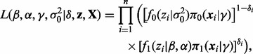
Methods: We propose a novel covariate-modulated local false discovery rate (cmfdr) that incorporates prior information about gene element–based functional annotations of SNPs, so that SNPs from categories enriched for non-null associations have a lower fdr for a given value of a test statistic than SNPs in unenriched categories. This readjustment of fdr based on functional annotations is achieved empirically by fitting a covariate-modulated parametric two-group mixture model. The proposed cmfdr methodology is applied to a large Crohn’s disease GWAS.

Results: Use of cmfdr dramatically improves power, e.g. increasing the number of loci declared significant at the 0.05 fdr level by a factor of 5.4. We also demonstrate that SNPs were declared significant using cmfdr compared with usual fdr replicate in much higher numbers, while maintaining similar replication rates for a given fdr cutoff in de novo samples, using the eight Crohn’s disease substudies as independent training and test datasets.

Availability an implementation: https://sites.google.com/site/covmodfdr/

Contact: wes.stat@gmail.com

Supplementary information: Supplementary data are available at Bioinformatics online.

1 INTRODUCTION

Large-scale hypothesis testing has emerged as a critical component of genetic analysis with the advent of high-throughput microarrays (Efron and Tibshirani, 2002). For example, it is now possible to survey a large number of single nucleotide polymorphisms (SNPs) across the entire genome in an attempt to locate genetic variations associated with trait variability or disease risk. An advantage of large-scale genome-wide association studies (GWAS) is the ability to discover the potential effect of any number of variants across the genome, without making strong a priori hypotheses about the subset of the genome to consider (Risch and Merikangas, 1996). A disadvantage is that a large number of false positives may occur when many hypothesis tests are conducted simultaneously (Devlin and Roeder, 1999). Consequently, modern GWAS have adopted a stringent Bonferroni-derived multiple testing threshold of for declaring individual SNP associations significant. Unfortunately, these GWAS have largely failed to identify substantial portions of the genetic basis of highly heritable diseases and complex traits (Collins, 2010; Manolio et al., 2009). Recent work has strongly suggested this could be because many genetic variants, each with individually small effects, compose their genetic architecture, limiting the power of GWAS to detect true associations, given currently obtainable sample sizes (Yang et al., 2010). This scenario is especially damaging to power if all SNPs are treated as a priori exchangeable and hence equally likely to be related to the phenotype of interest, an implicit assumption of Bonferroni thresholds and false discovery rate (FDR) control (Benjamini and Hochberg, 1995).

Other work has placed an emphasis on characterizing the biological function of genetic variants across the genome (Torkamani et al., 2011). Typically, this work has focused on understanding how differences in the protein-coding region of genes may damage or alter the corresponding protein structure. However, recent efforts have attempted to characterize the potential effect of variants within non-coding elements, which may alter the timing, amount or location of gene expression (ENCODE Consortium, 2012). Emerging from this research is a picture of widespread heterogeneity in the potential biological functionality of variants across the genome. A number of researchers have suggested that this heterogeneity of function translates to association studies, with certain genetic elements or categories of variants containing more or less trait-associated variants (Hindorff et al., 2009; Schork et al., 2013; Smith et al., 2011; Yang et al., 2011). Given this, it is potentially of use to leverage functional annotations or other locus-specific covariates to improve gene discovery and replication of associations in de novo samples.

Classical multiple-comparison procedures, such as the Bonferroni correction, control the family-wise error rate (FWER) or the probability of committing one or more Type I errors in a family of hypothesis tests. These procedures tend to be underpowered in large-scale testing paradigms (Efron, 2007). In other words, FWER procedures can be excessively conservative when thousands or millions of cases are tested. Benjamini and Hochberg (1995) proposed an alternative approach to Type I error control termed the FDR, defined as the expected proportion of errors among the rejected hypotheses. Variants of their algorithm are applied to P-values of test statistics (null hypothesis tail probabilities) from many tests to control FDR to a specified level under various conditions. Efron and Tibshirani (2002) developed an extension of FDR called the local false discovery rate (fdr) from an empirical Bayes point of view, defining fdr as the posterior probability that the null hypothesis is true, given the observed test statistic. The empirical Bayes approach to fdr is closely related to the Benjamini and Hochberg (1995) algorithm for FDR control (Efron and Tibshirani, 2002).

These groundbreaking methodologies for controlling multiplicity under large-scale hypothesis testing have received widespread attention and development (Brown et al., 2005; Efron, 2007; Ferkingstad et al., 2008; Genovese et al., 2002; Lawyer et al., 2009; Lewinger et al., 2007; Miller et al., 2001; Ploner et al., 2006; Sun et al., 2006; Tusher et al., 2001). Lewinger et al. (2007) proposed a mixture model of non-central test statistics, where the probability of being associated with a phenotype (having a non-centrality parameter different from zero) depends on multiple covariates. Ferkingstad et al. (2008) proposed an estimator that allows for modulating the fdr of each null hypothesis based on external covariates. If fdr depends on levels of a measured covariate, then the exchangeability assumption implicit in the definition of fdr is not optimal, and sizeable gains in power can be realized by accounting for this dependence (Efron, 2010; Sun et al., 2006). The key technique to account for the dependence of fdr on the covariate in the approach of Ferkingstad et al. (2008) was to bin the data into sets according to ordered values of . The assumption was that the influence of on the posterior probability is nearly constant in each bin if bins are small enough (in practice, to 20). The fdr is then estimated in each bin, possibly with smoothing across the bins. This approach works best for one covariate and becomes impractical as the number of covariates increases. It has been applied to large-scale testing of neuroimaging data (Lawyer et al., 2009).

In prior work, we have developed a scheme to assign gene element–based functional annotations for SNPs genome-wide, which takes into account the locus–locus correlations [linkage disequilibrium (LD)] that GWAS depend on for whole genome coverage (Schork et al., 2013). This LD-weighted annotation scheme provides multiple scores for each SNP in several genic categories, including exon, intron, 5′ untranslated regions (5′UTR) and 3′ untranslated region (3′UTR). Scores incorporate not only the category of a given variant but also the categories of all variants for which it is in LD (correlated with). Intergenic SNPs are defined as having zero scores in all functional categories and being >100 kb away from a protein-coding gene, providing a hypothesized ‘null’ collection. Using these functional annotations and summary statistics from 14 large GWAS, we showed that test statistics resulting from SNPs that are in LD with the 5′UTR of genes show the largest abundance of associations, while SNPs in LD with exons and the 3′UTR are also enriched. SNPs in LD with introns are modestly enriched and intergenic SNPs show a depletion of associations, relative to the average SNP (Schork et al., 2013). A more detailed description of how the LD-weighted genic annotations were produced is given in the Supplementary Materials.

This situation is illustrated in Fig. 1, which displays Q–Q plots of transformed P-values from a GWAS of Crohn’s Disease (CD) of 51 109 subjects, obtained through a publicly accessible database (Franke et al., 2010). Enrichment for true associations is expressed as a leftward deflection of the Q–Q plots stratified by genic category, representing an overabundance of low P-values compared with that expected under the global null hypothesis of no associations. Leftward deflections are directly related to decreased fdr for a given P-value threshold. The 5′UTR SNPs are most enriched, followed by exons, 3′UTR and introns. Intergenic SNPs are impoverished for true effects. These results were consistent across all assessed phenotypes (Schork et al., 2013) and strongly suggest that all SNPs should not be treated as a priori exchangeable for purposes of hypothesis testing but that certain categories are much more likely to show an association.

Fig. 1.

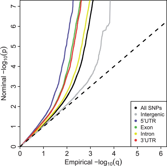
Q–Q plot of enrichment by functional annotation category for CD. The x-axis displays − transformed empirical P-values, and the y-axis the - transformed nominal P-values

The current article leverages the information available in genic annotation categories for large-scale GWAS hypothesis testing by presenting a novel, fully Bayesian approach for generalized covariate-modulated local false discovery rate (cmfdr) estimation, implemented using a Markov chain Monte Carlo (MCMC) sampling algorithm. Through this approach, we are able to model the influence of a vector of covariates on the distribution of the test statistics and hence on the fdr. Section 2 gives a brief review of fdr (Efron and Tibshirani, 2002) and introduces cmfdr, constructed from a Bayesian two-group mixture model that incorporates covariates. Section 3 presents the MCMC algorithm for fitting the model and drawing inferences and applies cmfdr to examples involving both simulated and real data. The last section is devoted to a discussion of results and future work.

2 METHODS

Review of fdr

Efron and Tibshirani (2002) made the assumption that the test statistic z_i, , has a different distribution based on whether the null hypothesis is true or false, where n is the total number of tests (SNPs). The non-null distribution will tend to have more extreme values of the test statistic. Hence, z_i follows a two-group mixture model

(1)

where is the proportion of true null hypotheses, is the proportion of true non-null hypotheses, f₀ is the probability density function if is true and f₁ is the probability density function if is false. Local false discovery rate (fdr) is the posterior probability that the i^th test is null given z_i, which by Bayes rule is given by

(2)

The null density was assumed to be standard normal (theoretical null) or normal with mean and variance estimated from the data (empirical null). The mixture density was estimated by fitting a high-degree polynomial to histogram counts (Efron, 2010). If a set of SNPs are selected with an estimated fdr for some , then we expect that on average of these will be true non-null SNPs.

Covariate-modulated fdr

A set of external covariates observed for each hypothesis test may influence the distribution of the test statistic (Efron, 2010; Sun et al., 2006). Under this scenario, incorporating the covariate effects into fdr estimation can dramatically increase power for gene discovery. For example, the distribution of GWAS z-scores may depend on SNP-level functional annotations (Schork et al., 2013), pleiotropic relationships with related phenotypes (Andreassen et al., 2013a, b), gene expression levels in certain tissues, evolutionary conservation scores and so forth. These external covariates can be used to break the exchangeability assumption implicit in Equation (1) and potentially increase the power for gene discovery over using standard fdr given in Equation (2).

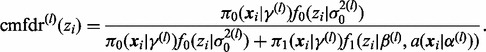
Let , where denotes an -dimensional vector of covariates (including intercept) for the i^th SNP. The cmfdr is defined as

(3)

where is the prior probability that the i^th test is non-null given and is the non-null density of z_i given . By Bayes’ rule, cmfdr is the posterior probability that the i^th test is null given both z_i and . We assume that the density under the null hypothesis does not depend on covariates. Both the probability of null status and the non-null density are allowed to depend on covariates, as described below.

Central to the estimation of the null proportion is the assumption that is large (say>0.90) and that the vast majority of SNPs with test statistics close to 0 are in fact null. These assumptions are reasonable for GWA data (Hon-Cheong et al., 2010).

A Bayesian Two-group model

Summary statistics from GWAS are often made publicly available only as 2-tailed P-values, and hence, the magnitude of the z score is recoverable but not the sign. Moreover, the sign of the z score is a result of arbitrary allele coding. Hence, we formulate the mixture model for the absolute z-scores. The extension of our method to signed z-scores is straightforward.

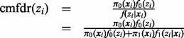
Folded normal-gamma mixture model

The distribution of z under is assumed to have the folded normal distribution, with null density , where is the normal density with mean 0 and standard deviation σ₀, and is an indicator function that takes the value 1 when and 0 otherwise. The density of z under the alternative hypothesis is assumed to have a gamma distribution with shape parameter and rate parameter β. Figure 2 gives a graphic presentation of these distributions. We chose a parametric non-null density for computational efficiency in modeling the effects of covariates. Parametric estimates of the non-null density also potentially provide more power than non-parametric estimates. We chose the gamma density because of its flexible shape and ability to model right-skewed heavy-tailed distributions.

Fig. 2.

Null and non-null distibutions. Mixture model Equation (1) consists of weighted mixture of folded normal (dotted line) and gamma densities (solid line)

Covariates are allowed to modulate the shape parameter of the gamma distribution

where = {}^T is an unknown parameter vector. The rate parameter is an unknown scalar not depending on . While it is possible to model the rate parameter as a function of , we have found that this leads to poor model convergence in the sampling algorithm, perhaps because of the lack of identifiability with other model parameters.

Additionally, we specify a location parameter to bind the non-null gamma densities away from zero. The ‘zero assumption’ of Efron (2007) states that the central peak of the z-scores consists primarily of null cases. Such an assumption is necessary to make the non-null distribution identifiable and for the MCMC sampling algorithm to converge. The assumption that the vast majority of SNPs with z-scores close to 0 are null is already commonly made in GWAS. Hence, we set the location parameter in the gamma distribution, corresponding to the median of the null density f₀. All SNPs with absolute z-scores <0.68 are thus a priori considered null.

We complete the mixture model formulation by positing a latent indicator vector , where if the i^th SNP is non-null and 0 otherwise. Then is the prior probability that given covariates . The dependence of on is modeled via a logistic regression

where is a vector of unknown parameters. The augmented likelihood function is then given by

(4)

where 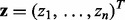is the vector of test statistics and is the design matrix. Integrating out the latent indicators gives the mixture model corresponding to Equation (3).

Prior distributions

We apply weakly informative priors to unknown parameters :

(5)

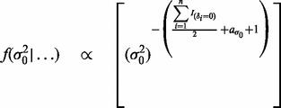
where and have large values on the diagonal, a₀ and b₀ are shape and rate parameters of gamma distribution and and are shape and scale parameters of inverse gamma distribution, respectively. Hyperparameters are fixed by the user. In the applications below, we set the dispersion matrices and to be diagonal with variance 10 000; and were both set to (0.001,0.001).

Sampling scheme

We sample the parameters , , and in turn from their full conditional distributions via a Gibbs sampler using Metroplis–Hastings (M-H) steps. Combining (4) and (5), the full conditional distributions are given as follows:

(6)

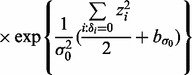where is an indicator function, and denotes the probability density of a parameter conditional on all other parameters and the data. The full conditional posteriors for and in (6) do not take standard forms and are sampled using a multiple-try M-H sampler (Givens and Hoeting, 2005) with a multivariate t-distribution candidate. The full conditional for β has a gamma distribution and for an inverse gamma distribution, so that both can be sampled directly. Each iteration of the Gibbs sampler also includes generation of , with a Bernoulli full conditional distribution. For

We can obtain an a posteriori estimate of cmfdr(z_i) for each z_i as follows. Assume we have L draws from the posterior distribution of the parameters. For each draw l,

Then, for example, the posterior median of cmfdr(z_i) can be estimated by taking the median of across all L posterior draws. The algorithm has been implemented in the R statistical package and is available at https://sites.google.com/site/covmodfdr/.

3 RESULTS

Simulation

We simulated phenotypes under different settings of generative parameters from real genotype data available for n = 3719 healthy individuals. For each permutation of simulation settings, we generated 100 unique phenotypes. We restricted our simulations to chromosome 1 (N = 191 128 SNPs) for computational efficiency, assuming it was representative of the whole genome. These simulations allow us to evaluate the performance of our method in scenarios that approximate realistic GWAS conditions, including correlated SNPs according to true LD patterns. A detailed description of the simulations and an expanded table including comparisons with the methods of Efron (2007) and Lewinger et al. (2007) are given in the Supplementary Materials.

Table 1 displays the median number of SNPs rejected and the false discovery proportion (FDP), or the proportion of rejected SNPs not in LD with a causal SNP. The cmfdr performs reasonably well across enrichment settings for more highly polygenic phenotypes, rejected SNPs conservatively for , but becoming progressively worse at controlling the FDP for phenotypes with low . The fdr of Efron (2007) controls the FDP at similar levels but also has less power than cmfdr (Supplementary Table S5). The mixture model of Lewinger et al. (2007) rejects more SNPs than either fdr or cmfdr, but also exhibits considerably higher FDP across the range of polygenicity levels. In particular, their model is unstable for null GWAS.

Table1.

Simulation study results

	Enr.	Strat.	Rejected	FDP
0.00	None	None	1 [0,5]	1.00 [0.00,1.00]
0.00	None	Low	4 [0,15]	1.00 [0.00,1.00]
0.001	None	None	79 [45,137]	0.25 [0.11,0.42]
0.001	None	Low	19 [4,70]	0.55 [0.19,0.79]
0.001	Low	None	92 [62,149]	0.30 [0.00,0.46]
0.001	Low	Low	17 [4,77]	0.44 [0.00,0.70]
0.001	High	None	90 [63,132]	0.28 [0.13,0.41]
0.001	High	Low	17 [5,47]	0.46 [0.21,0.67]
0.01	None	None	7 [1,19]	0.00 [0.00,0.17]
0.01	None	Low	6 [1,18]	0.25 [0.00,0.85]
0.01	Low	None	43 [17,101]	0.10 [0.00,0.20]
0.01	Low	Low	9 [1,38]	0.23 [0.00,0.67]
0.01	High	None	60 [16,124]	0.11 [0.00,0.23]
0.01	High	Low	8 [1,28]	0.14 [0.00,1.00]
0.05	None	None	4 [0,17]	0.00 [0.00,0.17]
0.05	None	Low	4 [0,15]	0.00 [0.00,1.00]
0.05	Low	None	39 [8,106]	0.00 [0.00,0.07]
0.05	Low	Low	8 [2,25]	0.00 [0.59,0.23]
0.05	High	None	47 [18,101]	0.00 [0.00,0.07]
0.05	High	Low	8 [1,27]	0.00 [0.00,0.23]

Note: Median number of SNPs rejected (Rejected) and FDP for the proposed cmfdr methodology. Settings include level of polygenicity (), level of covariate enrichment (Enr.) and level of population stratification (Strat.). Numbers in brackets give middle 95% of distributions across 100 simulations for each setting. A SNP was rejected if its cmfdr was . Details of simulation settings and more extended comparisons are given in the Supplementary Materials.

Real data application

The data consist of n = 942 772 SNP summary test statistics (SNP z-scores) from a GWAS meta-analysis of eight substudies of CD on subjects (6333 cases), obtained through a publicly accessible database (Franke et al., 2010). CD is a type of inflammatory bowel disease that is caused by multiple factors in genetically susceptible individuals. For this example, we selected the five SNP annotations from Schork et al. (2013) displayed in Fig. 1 to serve as covariates: intron, exon, 3′UTR, 5′UTR and intergenic; all annotation scores with the exception of Intergenic were first log transformed. These were entered together into the covariate-modulated mixture model, with the empirical null setting. The MCMC algorithm was run for 25 000 iterations with 20 000 retained draws. Plots of posterior draws showed convergence to stable posterior distributions for all parameters. Figure 3 shows the histogram of z-scores (all cases), the null subdensity and the posterior median fit of the mixture density. The estimated overall non-null proportion is 0.014. The fdr for each z-score is given by the height of the null subdensity at that score divided by the height of the mixture density. The parameter estimates are shown in Table 2. The 3′UTR and 5′UTR categories are associated with higher values of the shape parameter (and hence higher variance). Intron, exon, 3′UTR and 5′UTR are all associated with higher probability of non-null status. In contrast, intergenic SNPs are associated with higher values of the shape parameter and much lower probability of non-null status (0.001 non-null proportion for intergenic SNPs compared with the overall ). The positive coefficient for intergenic SNPs is a reflection of this sparsity because intergenic SNPs require more extreme z-scores than genic SNPs to obtain a high-posterior probability of being non-null.

Fig. 3.

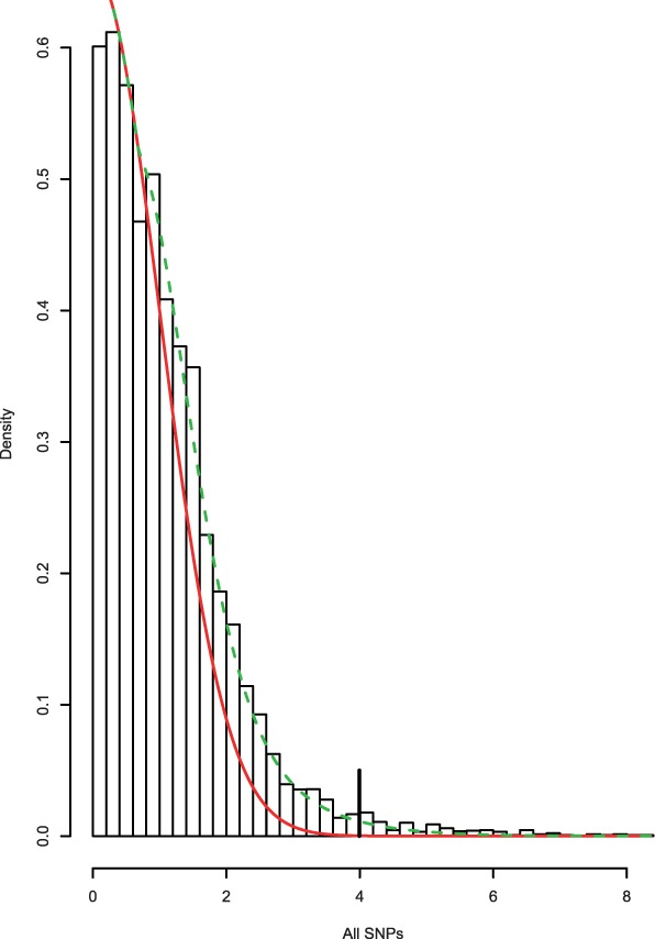
Histogram of CD absolute z-scores. Solid line gives estimated null subdensity , where was set to the sample mean. Dashed line gives estimated overall mixture model . The fdr for each z score is given by the height of the null subdensity at that score, divided by the height of the mixture density. Local FDR for z-scores >4.05 (vertical bar)

Table 2.

Parameter estimates with 95% posterior credible intervals from CD GWAS

Parameters
Intercept	0.33 [0.45,0.57]	−4.58 [−4.81,−4.35]
Intron	−0.04 [−0.01,0.01]	0.22 [0.17,0.27]
Exon	−0.13 [−0.16,−0.10]	0.82 [0.76,0.89]
3′UTR	0.05 [0.02,0.08]	0.27 [0.21,0.34]
5′UTR	0.23 [0.17,0.28]	0.40 [0.31,0.50]
Intergenic	0.77 [0.56,0.98]	−2.4 [−2.83,−1.97]
Rate parameter ()	1.50 [1.48,1.53]

Note: All estimates are presented in the form of median [95% credible interval].

Figure 4 compares the number of non-null SNPs rejected using usual fdr (Efron, 2007), and cmfdr with the five annotation categories. cmfdr rejected far more SNPs than fdr (Efron, 2007). For example, for a 0.05 cutoff, cmfdr rejects 3194 SNPs, whereas fdr rejects only 592, a factor of 5.4 times as many rejected SNPs. These 3194 SNPS consisted of 108 independent loci (leading SNP cmfdr and >1 Mb apart from each other). Of these 108 independent loci, 66 had been previously described in Franke et al. (2010). Franke et al. (2010) described an additional five loci that were not discovered using a 0.05 cutoff; however, in our analysis, each of these loci had a cmfdr . We found 42 novel loci where the leading SNP had a cmfdr . Reporting these findings as discoveries in accordance with the best practices in GWAS would require replication in an independent sample and a detailed characterization of their biological significance, both of which are beyond the scope of this article. However, to demonstrate that our proposed method identifies plausible candidate SNPs that might warrant this further investigation, we undertook a pleiotropy analysis. Given that CD is known to share etiology, including pleiotropic genetic factors (Cho and Brant, 2011) with ulcerative colitis, it is likely that causal SNPs would show joint associations. We found significant enrichment for nominal associations () with ulcerative colitis (Anderson et al., 2011) for both the 71 previously discovered loci (Bonferroni adjusted hypergeometric ) and the 42 novel loci (Bonferroni adjusted hypergeometric ). A complete list of previously discovered and novel gene names is given in the Supplementary Materials.

Fig. 4.

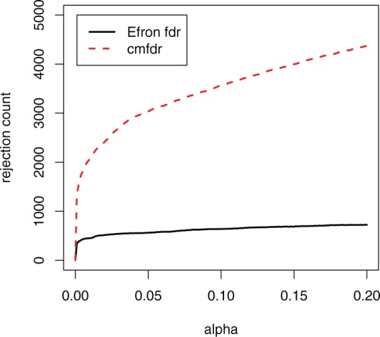
Power of fdr versus cmfdr. The x-axis is the cutoff to declare SNPs significant; the y-axis is number of rejected SNPs times 1-nominal fdr. The solid line indicates the number of SNPs rejected for usual fdr (Efron, 2007) using empirical null. The dashed line indicates the number of SNPs rejected using cmfdr with empirical null. SNPs not pruned for LD

We performed further analyses on CD substudies to determine whether this observed increase in the number of loci declared significant translates to increased number of replicating SNPs in de novo samples. The CD meta-analysis was composed of summary statistics from eight substudies (Franke et al., 2010). We computed z-scores from each of the 70 possible combinations of four substudies, leaving the z-scores computed from the remaining four independent substudies as test samples. We then estimated fdr and cmfdr for each training sample. For a given fdr cutoff, we determined the number of SNPs that replicated in the test sample. Replication was defined as one-sided and with the same sign as the corresponding z score in the training sample.

Number of replicated SNPs was much higher using cmfdr compared with fdr. For example, for usual fdr there was an average of 365 replicated SNPs (94.6% of SNPs declared significant) with an fdr cutoff of 0.05 in the training sample. In contrast, with the same cutoff using cmfdr, there was an average of 2956 SNPs (92.5% of declared significant SNPs) that replicated according to this definition, or almost 8.1 times as many SNPs. Similar increases in the number of replicated SNPs was observed for other cutoffs in the range. The larger number of SNPs declared significant for cmfdr compared with usual fdr largely remained when matched with empirical replication rates rather than nominal fdr threshold. For example, there was an average of 339 SNPs declared significant using usual fdr with an empirical replication rate of 0.95, compared with 2769 using cmfdr, or 8.2 times as many SNPs. In general, and in contrast to some of the simulation settings, replication rates were close to nominal for both usual fdr and cmfdr, across a range of cutoffs.

4 DISCUSSION

Methods for large-scale hypothesis testing that control Type I error rates without being overly conservative are crucial in GWAS (Efron, 2007; Franke et al., 2010). It has become increasingly evident that many complex phenotypes and diseases have many genetic determinants, each with small effect (Yang et al., 2010). Hence, traditional FWER correction is too conservative and severely underpowered. FDR (Benjamini and Hochberg, 1995) and fdr (Efron and Tibshirani, 2002) have come to be accepted broadly as routine techniques to control for the rate of false positive in large-scale hypothesis testing settings in a number of fields. However, even these methods do not account for the vast majority of phenotypic variance explained by common variants (Andreassen et al., 2013b). A problem with these and other multiple testing methods is that all SNPs are treated as exchangeable. In particular, each SNP is given the same a priori probability of being non-null. On the contrary, we (Schork et al., 2013) and others (Hindorff et al., 2009; Smith et al., 2011; Yang et al., 2011) have shown that the functional role of SNPs has a strong impact on the probability of association across a broad array of complex phenotypes and diseases.

This work proposes a novel Bayesian approach (cmfdr) to incorporate a set of important covariates into the fdr under a heteroscedastic model, where the probability of non-null status and the distribution of the test statistic under the non-null hypothesis are both modulated by covariates. The primary advantage of our methodology over traditional fdr methods is that two SNPs with the same z score can have different values of cmfdr if one is in a more enriched category than the other. Hence, by using SNP annotations to modulate fdr, more SNPs can be discovered for a given level of fdr control. In other words, methods such as cmfdr that break the exchangeability assumption are potentially more powerful than traditional fdr methods that assume exchangeability. In the CD example, we discovered 5.4 times as many SNPs (unpruned) using cmfdr compared with usual fdr for an identical 0.05 cutoff. The increase in number of replicated SNPs in de novo subsamples from fdr to cmfdr was even more dramatic. Parameter estimates of covariates can also be biologically informative about the relative functionality of different biological classifications of variants.

It is crucial to note that our LD-weighted SNP annotations were computed independently of the phenotypes investigated. Thus, modifying the fdr based on information from genic categories does not bias results toward rejecting more null hypotheses. Moreover, the cmfdr methodology is capable of handling any relevant source of information, including, for example, pleiotropic relationships of SNPs with multiple phenotpyes (Andreassen et al., 2013a, b), gene expression levels in various tissues and evolutionary conservation scores, among others.

The proposed methodology has some drawbacks. First, as currently formulated, it assumes all hypothesis tests are independent. This is not true for SNPs in LD, and our 95% credible intervals are probably too small. Moreover, it remains unclear what impact LD has on FDP control because it may be the case that all or almost all ‘tag SNPs’ are in partial LD with causal SNPs but are not themselves causal. Correlation across SNPs can be handled, for example, by repeatedly and randomly pruning SNPs for independence before running the MCMC algorithm, by using a discrete Markov random field formulation (Li et al., 2010) or by modeling SNPs simultaneously using, for example, a multivariate mixed-effects model framework (Carbonetto and Stephens, 2013). We have implemented a random pruning option available with the R code distribution. Second, it may be the case for some applications that the gamma distribution does not fit the tail probabilities of the non-null distribution well. We have used other distributions (e.g. the skewed generalized normal) and are currently developing a non-parametric alternative that produces flexible fits to tail probabilities. Although non-parametric estimates of the non-null density avoid bias from lack of model fit, parametric alternatives can be more powerful if the fit is adequate. Finally, it appears from simulations that the cmfdr methodology can be overly liberal in scenarios where is close to 0. Care must therefore be taken when applying cmfdr in these circumstances.

REFERENCES

- Anderson CA, et al. Meta-analysis identifies 29 additional ulcerative colitis risk loci, increasing the number of confirmed associations to 47. Nat. Genet. 2011;43:246–252. doi: 10.1038/ng.764. [DOI] [PMC free article] [PubMed] [Google Scholar]
- Andreassen OA, et al. Improved detection of common variants associated with schizophrenia by leveraging pleiotropy with cardiovascular disease risk factors. Am. J. Hum. Genet. 2013a;7:197–209. doi: 10.1016/j.ajhg.2013.01.001. [DOI] [PMC free article] [PubMed] [Google Scholar]
- Andreassen OA, et al. Improved detection of common variants associated with schizophrenia and bipolar disorder using pleiotropy-informed conditional False Discovery Rate method. PLoS Genet. 2013b;9:e1003455. doi: 10.1371/journal.pgen.1003455. [DOI] [PMC free article] [PubMed] [Google Scholar]
- Benjamini Y, Hochberg Y. Controlling the false discovery rate: a practical and powerful approach to multiple testing. J. R. Stat. Soc. Ser. B. 1995;57:289–300. [Google Scholar]
- Brown L, et al. Statistical analysis of a telephone call center: a queueing-science perspective. J. Am. Stat. Assoc. 2005;100:36–50. [Google Scholar]
- Carbonetto P, Stephens M. Integrated enrichment analysis of variants and pathways in genome-wide association studies indicates central role for IL-2 signaling genes in type 1 diabetes, and cytokine signaling genes in Crohn’s Disease. PLoS Genet. 2013;9:e1003770. doi: 10.1371/journal.pgen.1003770. [DOI] [PMC free article] [PubMed] [Google Scholar]
- Cho JH, Brant SR. Recent insights into the genetics of inflammatory bowel disease. Gastroenterology. 2011;140:1704–1712. doi: 10.1053/j.gastro.2011.02.046. [DOI] [PMC free article] [PubMed] [Google Scholar]
- Collins F. Has the revolution arrived? Nature. 2010;464:674–675. doi: 10.1038/464674a. [DOI] [PMC free article] [PubMed] [Google Scholar]
- Devlin B, Roeder K. Genomic control for association studies. Biometrics. 1999;55:997–1004. doi: 10.1111/j.0006-341x.1999.00997.x. [DOI] [PubMed] [Google Scholar]
- Efron B. Size, power and false discovery rates. Ann. Stat. 2007;35:1351–1377. [Google Scholar]
- Efron B. Large-Scale Inference: Empirical Bayes Methods for Estimation, Testing, and Prediction. Cambridge: Cambridge University Press; 2010. [Google Scholar]
- Efron B, Tibshirani R. Empirical bayes methods and false discovery rates for microarrays. Genet. Epidemiol. 2002;23:70–86. doi: 10.1002/gepi.1124. [DOI] [PubMed] [Google Scholar]
- The ENCODE Consortium. An integrated encyclopedia of DNA elements in the human genome. Nature. 2012;489:57–74. doi: 10.1038/nature11247. [DOI] [PMC free article] [PubMed] [Google Scholar]
- Ferkingstad E, et al. Unsupervised empirical bayesian multiple testing with external covariates. Ann. Appl. Stat. 2008;2:714–735. [Google Scholar]
- Franke A, et al. Genome-wide meta-analysis increases to 71 the number of confirmed Crohn’s disease susceptibility loci. Nat. Genet. 2010;42:1118–1125. doi: 10.1038/ng.717. [DOI] [PMC free article] [PubMed] [Google Scholar]
- Genovese CR, et al. Thresholding of statistical maps in functional neuroimaging using the false discovery rate. Neuroimage. 2002;15:870–878. doi: 10.1006/nimg.2001.1037. [DOI] [PubMed] [Google Scholar]
- Givens GH, Hoeting JA. Computational Statistics. Vol. 483. Hoboken, NJ, USA: Wiley-Interscience Press; 2005. [Google Scholar]
- Hindorff LA, et al. Potential etiologic and functional implications of genome-wide association loci for human diseases and traits. Proc. Natl Acad. Sci. USA. 2009;106:9362–9367. doi: 10.1073/pnas.0903103106. [DOI] [PMC free article] [PubMed] [Google Scholar]
- Hon-Cheong H, et al. Estimating the total number of susceptibility variants underlying complex diseases from genome-wide association studies. PloS One. 2010;5:e13898. doi: 10.1371/journal.pone.0013898. [DOI] [PMC free article] [PubMed] [Google Scholar]
- Lawyer G, et al. Local and covariate-modulated false discovery rates applied in neuroimaging. Neuroimage. 2009;47:213–219. doi: 10.1016/j.neuroimage.2009.03.047. [DOI] [PubMed] [Google Scholar]
- Lewinger JP, et al. Hierarchical Bayes prioritization of marker associations from a genome-wide association scan for further investigation. Genet. Epidemiol. 2007;31:871–883. doi: 10.1002/gepi.20248. [DOI] [PubMed] [Google Scholar]
- Li H, et al. A hidden Markov random field model for genome-wide association studies. Biostatistics. 2010;11:139–150. doi: 10.1093/biostatistics/kxp043. [DOI] [PMC free article] [PubMed] [Google Scholar]
- Manolio TA, et al. Finding the missing heritability of complex diseases. Nature. 2009;461:747–753. doi: 10.1038/nature08494. [DOI] [PMC free article] [PubMed] [Google Scholar]
- Miller CJ, et al. Controlling the false discovery rate in astrophysical data analysis. Astron. J. 2001;122:3492–3505. [Google Scholar]
- Ploner A, et al. Multidimensional local false discovery rate for microarray studies. Bioinformatics. 2006;22:556–565. doi: 10.1093/bioinformatics/btk013. [DOI] [PubMed] [Google Scholar]
- Risch N, Merikangas K. The future of genetic studies of complex human diseases. Science. 1996;255:1516–1517. doi: 10.1126/science.273.5281.1516. [DOI] [PubMed] [Google Scholar]
- Schork AJ, et al. Genetic architecture of the missing heritability for complex human traits and diseases. PLoS Genet. 2013;9:e1003449. [Google Scholar]
- Smith EN, et al. Genome-wide association of bipolar disorder suggests an enrichment of replicable associations in regions near genes. PLoS Genet. 2011;7:e1002134. doi: 10.1371/journal.pgen.1002134. [DOI] [PMC free article] [PubMed] [Google Scholar]
- Sun L, et al. Stratified false discovery control for large-scale hypothesis testing with application to genome-wide association studies. Genet. Epidemiol. 2006;30:519–530. doi: 10.1002/gepi.20164. [DOI] [PubMed] [Google Scholar]
- Torkamani A, et al. Annotating individual human genomes. Genomics. 2011;98:233–241. doi: 10.1016/j.ygeno.2011.07.006. [DOI] [PMC free article] [PubMed] [Google Scholar]
- Tusher VG, et al. Significance analyses of microarrays applied to the ionizing radiation response. Proc. Natl Acad. Sci. USA. 2001;98:5116–5121. doi: 10.1073/pnas.091062498. [DOI] [PMC free article] [PubMed] [Google Scholar]
- Yang B, et al. Common SNPs explain a large proportion of the heritability for human height. Nat. Genet. 2010;42:565–569. doi: 10.1038/ng.608. [DOI] [PMC free article] [PubMed] [Google Scholar]
- Yang J, et al. Genome partitioning of genetic variation for complex traits using common SNPs. Nat. Genet. 2011;43:519–525. doi: 10.1038/ng.823. [DOI] [PMC free article] [PubMed] [Google Scholar]
Associated Data
This section collects any data citations, data availability statements, or supplementary materials included in this article.