Deformable segmentation of 3D MR prostate images via distributed discriminative dictionary and ensemble learning

Abstract

Purpose:

Automatic prostate segmentation from MR images is an important task in various clinical applications such as prostate cancer staging and MR-guided radiotherapy planning. However, the large appearance and shape variations of the prostate in MR images make the segmentation problem difficult to solve. Traditional Active Shape/Appearance Model (ASM/AAM) has limited accuracy on this problem, since its basic assumption, i.e., both shape and appearance of the targeted organ follow Gaussian distributions, is invalid in prostate MR images. To this end, the authors propose a sparse dictionary learning method to model the image appearance in a nonparametric fashion and further integrate the appearance model into a deformable segmentation framework for prostate MR segmentation.

Methods:

To drive the deformable model for prostate segmentation, the authors propose nonparametric appearance and shape models. The nonparametric appearance model is based on a novel dictionary learning method, namely distributed discriminative dictionary (DDD) learning, which is able to capture fine distinctions in image appearance. To increase the differential power of traditional dictionary-based classification methods, the authors' DDD learning approach takes three strategies. First, two dictionaries for prostate and nonprostate tissues are built, respectively, using the discriminative features obtained from minimum redundancy maximum relevance feature selection. Second, linear discriminant analysis is employed as a linear classifier to boost the optimal separation between prostate and nonprostate tissues, based on the representation residuals from sparse representation. Third, to enhance the robustness of the authors' classification method, multiple local dictionaries are learned for local regions along the prostate boundary (each with small appearance variations), instead of learning one global classifier for the entire prostate. These discriminative dictionaries are located on different patches of the prostate surface and trained to adaptively capture the appearance in different prostate zones, thus achieving better local tissue differentiation. For each local region, multiple classifiers are trained based on the randomly selected samples and finally assembled by a specific fusion method. In addition to this nonparametric appearance model, a prostate shape model is learned from the shape statistics using a novel approach, sparse shape composition, which can model nonGaussian distributions of shape variation and regularize the 3D mesh deformation by constraining it within the observed shape subspace.

Results:

The proposed method has been evaluated on two datasets consisting of T2-weighted MR prostate images. For the first (internal) dataset, the classification effectiveness of the authors' improved dictionary learning has been validated by comparing it with three other variants of traditional dictionary learning methods. The experimental results show that the authors' method yields a Dice Ratio of 89.1% compared to the manual segmentation, which is more accurate than the three state-of-the-art MR prostate segmentation methods under comparison. For the second dataset, the MICCAI 2012 challenge dataset, the authors' proposed method yields a Dice Ratio of 87.4%, which also achieves better segmentation accuracy than other methods under comparison.

Conclusions:

A new magnetic resonance image prostate segmentation method is proposed based on the combination of deformable model and dictionary learning methods, which achieves more accurate segmentation performance on prostate T2 MR images.

I. INTRODUCTION

Magnetic resonance (MR) imaging is increasingly considered one of the best imaging modalities for prostate-related clinical studies, particularly in assessing the extent and aggressiveness of prostate cancer.¹ Due to the fact that the traditional transrectal ultrasonography (TRUS)-guided biopsy has low sensitivity and provides limited information on the prostate anatomy, MR-guided transperineal prostate core biopsy^2,3 has become a preferred alternative for prostate cancer detection.⁴ To place the needle accurately during biopsy, accurate detection, localization, and characterization of cancer in the untreated and treated gland must first be achieved.^5,6 Accordingly, segmentation of the prostate gland is a fundamental step for automatically measuring or tracking the prostate structures in MR-guided prostate interventions.⁷ An accurate segmentation of the prostate gland^8,9 not only captures the volumetric properties of the prostate gland, but also facilitates image-based diagnosis and treatment tasks, such as prostate cancer staging and MR-guided radiotherapy planning.¹⁰ In the past decade, a large number of methods have been proposed for segmenting prostate MR images automatically.^11,12 However, the segmentation problem still remains a very challenging task especially in the prostate base and apex due to large appearance and shape variations of these parts in MR images. Accordingly, more extensive methods need to be developed for the automatic and accurate segmentation of the prostate in MR images.

I.A. Previous work and motivation

Among existing studies, multiatlas-based methods and deformable models are the two most popular approaches for MR prostate segmentation. In multiatlas-based methods,^13,14 each training image (atlas) is first registered to the target image together with its label map. Then, the selected warped label images are fused to derive the segmentation for the target image. In addition to MR prostate segmentation, numerous atlas-based segmentation methods have been applied in the segmentation of single brain structures, such as the hippocampus and ventricles,^15,16 as well as multiple brain regions simultaneously.^17,18 For instance, Coupé et al.¹⁵ and Rousseau et al.¹⁷ both proposed to use a patch-based nonlocal mean strategy for label propagation. This approach is able to avoid the use of computationally expensive nonrigid registration in the label propagation procedure, thus improving the efficiency of multiatlas-based methods. Wang et al.¹⁶ first estimated the correlations between different atlases (known as a linear appearance-label model) and then derived the optimal weights for label fusion. Asman and Landman¹⁸ used regional performance level estimations to formulate label fusion as a statistical modeling problem, which allows atlas images to be fused in a spatially varying manner. For MR prostate segmentation, Klein et al.¹² proposed to use localized mutual information as the similarity measure for atlas alignment and then compared the performance within majority voting and STAPLE frameworks for label fusion. Langerak et al.¹⁹ proposed a method called SIMPLE that combines propagated segmentations in atlas selection and performance estimation strategies. Liao et al.²⁰ proposed a hierarchical prostate MR segmentation method that performs multiatlas-based sparse label propagation at the coarse level and then a domain-specific semisupervised segmentation at the fine level. Furthermore, Liao et al.²¹ adopted a deep learning framework to learn features in a hierarchical and unsupervised way. The learned features are used in the sparse label propagation to derive accurate segmentations of the prostate in MR images. However, one common limitation of these multiatlas-based methods is it is difficult to perform atlas selection and label fusion if the target image is very different from all available atlases in terms of both shape and appearance. In addition, nonrigid registration is usually required for accurate segmentation, thus the computation time in the multiatlas-based methods increases significantly with the number of atlases used.

On the other hand, deformable model approaches become a natural choice for tackling the problem of prostate segmentation, as they inherently capture shape and appearance variations across a population. For example, Tsai et al.²² proposed to model the shape prior by principal component analysis on a set of signed distance representations and used it to increase the robustness of the model deformation. Martin et al.²³ proposed a 3D prostate MR segmentation method via multiatlas-based deformable modeling. They first built a probabilistic segmentation by atlas matching and then used the result to drive the deformable segmentation. Toth et al.²⁴ improved the traditional Active Shape Model (ASM) to segment the prostate from multiprotocol in vivo MRI/MRS by employing an automated MRS-based model initialization scheme and a multifeature appearance model to prevent the leaking problem on weak boundaries of MRI. Zhan and Shen²⁵ trained a set of Gabor support vector machines on different regions around the prostate boundary and integrated the tissue labeling results with surface deformation to derive the segmentation. To prevent boundary leakage, Kirschner et al.²⁶ presented a probabilistic ASM (PASM) which can adapt a statistical shape model to a larger subspace than the one spanned by the principal eigenvectors used in the standard ASM. Maan and Heijden.²⁷ employed the 3D AAM method for prostate segmentation following shape-context-based nonrigid surface registration. Finally, Toth et al.¹¹ proposed a landmarkfree AAM method based on level-set shape representations and further created a deformable registration framework for fitting a trained appearance model onto a new image by using multiple image-derived attributes.

Although the above-mentioned ASM/AAM-based methods have proved to be feasible approaches for automatic prostate MR segmentation, they all are subject to an inherent limitation: ASM/AAM assumes that both shape and appearance statistics of the target object follow a Gaussian distribution. Unfortunately, this assumption is not valid in prostate MR images due to (1) the complicated neighboring structures along the prostate boundary, (2) highly inhomogeneous magnetic fields, and (3) large interpatient variations, as shown in Fig. 1. Figure 1(a) gives one slice of a T2-weighted MR prostate image. Figures 1(b) and 1(c) show, respectively, the joint distribution of two appearance features (intensity and gradient) and the histogram of gradients for illustrating the interpatient appearance variations. Here, both features are normalized before computing their joint distribution. As we can see, the appearance distribution is complicated and does not follow a Gaussian distribution. This clearly explains the limitation of ASM/AAM, since their inherent assumption no longer holds. Figure 1(d) gives the interpatient shape variation, which does not follow Gaussian distribution. Figure 1(e) further shows several typical prostate shapes, indicating large interpatient shape variations. In this paper, we seek to avoid this Gaussian assumptions by using sparse learning methods for both appearance and shape modeling, which can better accommodate the large appearance and shape variations found in prostate MR images.

FIG. 1.

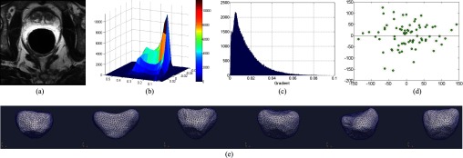
Complicated non-Gaussian distribution of appearance features in MR prostate images. (a) A typical slice of a T2-weighted MR prostate image. (b) Joint distribution of intensity and gradient of voxels within prostate regions across ten subjects. (c) The histogram of gradients within prostate regions across ten subjects. (d) Prostate shape distribution along the two major shape variation modes, corresponding to the two eigenvectors with the largest eigenvalues by PCA. (e) Shape models obtained for different patients, which demonstrates the large interpatient shape variations.

Our method is inspired by sparse learning theory, which has been comprehensively studied in the field of computer vision field for tasks such as face recognition²⁸ and image restoration.^29,30 Recently, sparse learning theory has also gained high attention in the field of medical image analysis, particularly in problems concerning image reconstruction³¹ and anatomical shape modeling.³² Instead of assuming any parametric model, sparse learning aims to learn a parameterfree dictionary to represent signals of the same class, thus opening a door to better model objects with complicated distributions of appearance, such as the prostate. However, dictionary learning does not aim to distinguish one class from others (i.e., prostate vs nonprostate), but simply represent all classes (i.e., prostate and nonprostate). In this context, in order to well differentiate prostate from nonprostate tissues, which may eventually affect the final segmentation accuracy, we propose to learn a sparse dictionary with increased ability of discrimination. In this way, we can relieve the assumption of Gaussian distribution of appearance inherent to ASM/AAM models, instead using sparse learning techniques to model image appearance in a nonparametric and discriminative manner.

I.B. Contributions of our work

In this paper, we improve the conventional sparse learning approach with discriminative techniques and further integrate it with deformable modeling for prostate segmentation. Specifically, the learned sparse dictionaries are used to identify prostate tissue from nonprostate tissue and then provide appearance cues for driving our deformable model to the prostate boundaries. To boost the discriminative power of the conventional sparse learning method in tissue identification, three strategies are proposed in our work. First, the dictionaries for both prostate and nonprostate tissues are constructed in a discriminative feature space by performing minimum redundancy maximum relevance (mRMR) feature selection.³³ Second, linear discriminant analysis (LDA) is further applied to the representation residuals from different dictionaries for optimal separation between prostate and nonprostate tissues. Third, to further improve the robustness of the above sparse representation-based classification, a set of local dictionaries is learned for tissue differentiation along the prostate boundary. Compared to the global dictionary, these local dictionaries can achieve better tissue differentiation by independently capturing small local appearance variations. Moreover, multiple classifiers are further trained for each local region to improve the overall classification performance. In the application stage, a particular sequence of local dictionaries is applied to each partition of the subject. Since multiple dictionaries may contribute to the labeling of the same area in the new subject image, a label fusion procedure is further performed to integrate multiple probability maps into the final labeling result, which provides effective appearance cues to robustly drive the deformable model onto the prostate boundary. Meanwhile, the deformed surface will be also constrained by the prostate shape prior built from sparse shape composition.³² Evaluations on the T2-weighted prostate MR images indicate that the proposed deformable model with discriminative dictionary learning yields the best segmentation performance in term of both accuracy and robustness when compared to both conventional deformable models and multiatlas-based methods.

The remainder of the paper is organized as follows. In Sec. II, we give the details of our proposed method. The conventional deformable model and its limitations regarding the Gaussian distribution assumption are presented in Sec. II A. To describe appearance and shape cues in a nonparametric way, we further propose our deformable model approach based on distributed discriminative dictionary and ensemble learning, outlined in Sec. II B. In Sec. III, we will present the evaluation results of our proposed method on prostate T2-weighted MR images, with comparison to other state-of-the-art methods. Section IV will give the discussion about our method as well as potential clinical analysis. Finally, we will provide a conclusion to this work in Sec. V.

II. METHOD

Our method aims to robustly segment the prostate gland in 3D T2-weighted MRI images by using both appearance and sparse shape models to drive a deformable model for segmentation. The appearance model is based on the proposed dictionary learning method, which can distinguish prostate voxels from nonprostate voxels via voxelwise classification. It is used as an external force to drive the deformable model. The shape model is obtained by sparse shape composition, a novel shape modeling method. It helps regularize the 3D surface deformation by constraining it to be always within the observed shape subspace.

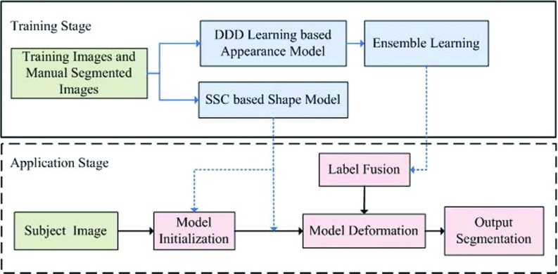
Figure 2 gives the schematic diagram of our deformable model framework. Similar to many other deformable model methods, it consists of two stages: a training stage and an application stage.

• •In the training stage, separate appearance and shape models are learned from a set of annotated training samples. Specifically, a set of distributed discriminative dictionaries is constructed using the method proposed in Sec. II B 1 to capture spatially adaptive appearance characteristics. In addition to the appearance model, a statistical shape model, introduced in Sec. II B 2, is also learned upon the shape instances through sparse shape composition.
• •In the application stage, we first infer an initial surface for the subject image using a landmark-based approach, which will be detailed in Sec. II B 3. Then, this initial shape is deformed with the guidance from the previously learned appearance and shape models. Multiple learned classifiers are fused to act as appearance guides to drive the deformable model onto the desired prostate boundary. The SSC-based shape prior is utilized to refine the deformable model at run-time. In the end, the final segmentation is obtained by iteratively deforming the model under guidance from both the appearance model and the shape model until convergence.

FIG. 2.

The schematic description of our deformable segmentation framework.

Before introducing our proposed method, we briefly review the conventional deformable model and especially its limitation of a Gaussian distribution assumption. Then, to address this limitation, we propose to represent both appearance and shape distributions using a sparse learning algorithm.

II.A. Conventional deformable model

In deformable segmentation of the prostate, a deformable model is often represented by a 3D shape or surface, i.e., with a triangle mesh of N vertices $\left\{{\mathit{v}}_i\right|i=1,...,N\}$, where ${\mathit{v}}_i$ denotes the ith vertex on the 3D surface. Each vertex in the deformable model iteratively evolves by merging information from both the image appearance model and the shape model. With well-designed appearance and shape models, surface deformation will converge at the prostate boundaries.

Mathematically, the evolution of a deformable model can be formulated as the minimization of an energy function E, which contains the external energy E_ext corresponding to the appearance model, and also the internal energy E_int corresponding to the shape model. Different deformable models have different definitions for the external energy E_ext and the internal energy E_int. Here, we take ASM, for example, and summarize its energy function as shown in Eq. (1),

$$E=E_{\mathrm{ext}}+{\lambda }_0{E}_{\mathrm{int}},$$ (1)

where the external energy E_ext attracts the surface toward the object boundary, and the internal energy E_int ensures the smoothness³⁴ and shape regularity³⁵ of the deformed surface.

Specifically, to build the external energy E_ext, each training image is first warped to the mean space for obtaining a “shape-aligned” patch. Then, the line profile on each vertex ${\mathit{v}}_i$ is scanned into vector ${\mathit{y}}_i$, and principal component analysis (PCA) is applied to build an appearance model for each vertex. Since ASM assumes a Gaussian distribution of the appearance model, a statistical model of the line profile at each vertex ${\mathit{v}}_i$ is estimated by its mean $\overline{{\mathit{y}}_i}$ and covariance matrix ${\mathbb{C}}_i^{\mathrm{profile}}$. The formulation of ASM aims to minimize the line profile differences between the mean model and the target sample. The external function E_ext is thereby given as the Mahalanobis distance between the target sample and the model mean as below

$$E_{\mathrm{ext}}=\sum _i{\left({\mathit{y}}_i-\overline{{\mathit{y}}_i}\right)}^{\mathrm{T}}{\mathbb{C}}_i^{\mathrm{profile}}\left({\mathit{y}}_i-\overline{{\mathit{y}}_i}\right).$$ (2)

Here, $\left({\mathit{y}}_i-\overline{{\mathit{y}}_i}\right)$ measures the difference between profiles of vertex ${\mathit{v}}_i$ on the current location and the mean appearance model.

Similarly, to build the internal energy E_int, all N vertices on each shape are concatenated as a long vector $\mathit{v}={\left[{\mathit{v}}_1^{\mathrm{T}},{\mathit{v}}_2^{\mathrm{T}},...,{\mathit{v}}_N^{\mathrm{T}}\right]}^{\mathrm{T}}$. The statistical shape model is then built by aligning all the training shapes into a common frame followed by PCA.³⁶ Specifically, the statistical shape model of the shape vector is estimated by the mean vector $\overline{\mathbf{v}}$ and covariance matrix ${\mathbb{C}}^{\mathrm{shape}}$ under the Gaussian assumption on the shape distribution

$$E_{\mathrm{int}}={\left(\mathit{v}-\overline{\mathbf{v}}\right)}^{\mathrm{T}}{\mathbb{C}}^{\mathrm{shape}}\left(\mathit{v}-\overline{\mathbf{v}}\right).$$ (3)

Here, $\left(\mathit{v}-\overline{\mathbf{v}}\right)$ measures the displacement of current shape v from the mean shape $\overline{\mathbf{v}}$.

Since E_ext and E_int measure the fitness on appearance and shape, respectively, the previous success of ASM mainly comes from the use of both appearance and shape priors. However, due to large variations and complicated distributions of prostate appearances and shapes in MR images [as shown in Fig. 1(b) with the non-Gaussian joint distribution of intensity and gradient of voxels and also in Fig. 1(d) with the non-Gaussian distribution of prostate shapes], the basic assumption of a Gaussian distribution is invalid, and thus the conventional ASM approach is not able to segment prostate MR images accurately.

To avoid the shortcomings of the Gaussian assumption, we propose to use sparse learning techniques to model both shape and appearance in a nonparametric way. In Sec. II B, we will first introduce how sparse learning is used in our work to model the external energy E_ext. Then, we will give our formulation of internal energy E_int by adopting sparse shape composition.³² Finally, our deformable model is summarized in Sec. II B 3.

II.B. Deformable model via distributed discriminative dictionary and ensemble learning

In this section, our aim is to develop a deformable segmentation method that is not limited to the Gaussian assumption of both appearance and shape models. We employ a dictionary learning method for building appearance and shape models in a nonparametric fashion. For the appearance model, we first introduce a standard dictionary learning method (i.e., global standard dictionary learning) as the basic model, which is less discriminative on separating prostate and nonprostate tissues. In order to improve the tissue differentiation power of the appearance model, we further use two other dictionary methods, global discriminative dictionary learning and distributed discriminative dictionary learning, for better discrimination between prostate and nonprostate tissue. For the shape model, to fully capture large shape variations of prostates, we adopt a recently developed sparse shape composition method³² for nonparametric shape modeling in the deformable segmentation. In this way, the shape details, which may be not statistically significant in the shape distribution, will be preserved, thus improving the segmentation accuracy.

II.B.1. Appearance modeling by dictionary learning

II.B.1.A. Global standard dictionary (GSD) learning

In sparse representation theory, data are modeled by a linear combination of few elements, also called as atoms. Each atom is chosen from an overcomplete dictionary, in which the number of atoms usually exceeds the dimension of the data space. To build the dictionary, one common method is to simply combine the repository of data. However, since the size of data is usually very large, making the computation of a sparse representation infeasible, the dictionary is usually learned by approximative dictionary learning methods, such as the K-SVD algorithm.³⁷ Therefore, given a dictionary $\mathit{D}\in {\mathbb{R}}^{M\times Q}$, which has Q atoms (each with M dimensions), the goal of sparse representation for a testing sample $\mathit{f}\in {\mathbb{R}}^M$ is to select a small number of atoms from D to best represent f. Mathematically, the sparse representation problem is formulated as the following minimization problem:

$$\mathit{\alpha }={\mathrm{argmin}}_{\mathit{\alpha }}{\Vert \mathit{f}-\mathit{D}\mathbf{\alpha }\Vert }_2^2+{\beta }_0{\Vert \mathit{\alpha }\Vert }_1.$$ (4)

Here, $\mathit{\alpha }\in {\mathbb{R}}^Q$ is a coefficient vector including the linear coefficients for the atoms in the dictionary D. ${\Vert \mathit{\alpha }\Vert }_1$ is an l₁ norm on $\mathit{\alpha }$ for guaranteeing the sparsity of $\mathit{\alpha }$. β₀ is the parameter that controls the number of nonzero elements (or sparsity) in $\mathit{\alpha }$. The number of nonzero elements in $\mathit{\alpha }$ decreases with the increase of the value of β₀. By solving Eq. (4), the testing sample f can be reconstructed by $\mathit{D}\alpha$. In our work, each training/testing sample f is represented by a 3D intensity patch centered at the underlying sampled voxel.

Based on the sparse representation, a specific task such as classification can be completed by properly learning the dictionaries. This kind of method is known as sparse representation based classification (SRC). Different from the “one-class representation” problem (i.e., describing the characteristics of only the prostate) as solved in the sparse representation problem in Eq. (4), the goal of SRC is to “distinguish” one class from others (i.e., prostate vs nonprostate). Therefore, the dictionary used in SRC is the combination of both positive and negative subdictionaries $\left\{{\mathit{D}}_{\mathrm{PR}},{\mathit{D}}_{\mathrm{NPR}}\right\}$, where ${\mathit{D}}_{\mathrm{PR}}\in {\mathbb{R}}^{M\times Q_{\mathrm{PR}}}$ and ${\mathit{D}}_{\mathrm{NPR}}\in {\mathbb{R}}^{M\times Q_{\mathrm{NPR}}}$ denote prostate and nonprostate subdictionaries, respectively. Each subdictionary is formed by grouping the intensity patches of training samples columnwise from each respective region (i.e., prostate and nonprostate).

For classification, the subdictionaries $\left\{{\mathit{D}}_{\mathrm{PR}},{\mathit{D}}_{\mathrm{NPR}}\right\}$ are jointly used to represent a new testing sample $\mathit{f}\in {\mathbb{R}}^M$. This sample is labeled as the class that best reconstructs it through sparse representation. By combining the subdictionaries to form a single global dictionary $\mathit{D}=\left[{\mathit{D}}_{\mathrm{PR}},{\mathit{D}}_{\mathrm{NPR}}\right]\in {\mathbb{R}}^{M\times \left(Q_{\mathrm{PR}}+Q_{\mathrm{NPR}}\right)}$, the sparse code of the new sample f can be solved as $\mathit{\alpha }\in {\mathbb{R}}^{Q_{\mathrm{PR}}+Q_{\mathrm{NPR}}}$ according to Eq. (4). Here $\mathit{\alpha }={\left[{\mathit{\alpha }}_{\mathrm{PR}}^{\mathrm{T}},{\mathit{\alpha }}_{\mathrm{NPR}}^{\mathrm{T}}\right]}^{\mathrm{T}}$, where $\left\{{\mathit{\alpha }}_{\mathrm{PR}},{\mathit{\alpha }}_{\mathrm{NPR}}\right\}$ carries the elements of $\mathit{\alpha }$, corresponding to the indices of columns belonging to $\left\{{\mathit{D}}_{\mathrm{PR}},{\mathit{D}}_{\mathrm{NPR}}\right\}$ in D.

Then the reconstruction residual of sample feature f with respect to each class can be calculated as follows:

$${\mathit{r}}_{\mathrm{PR}}=\mathit{f}-{\mathit{D}}_{\mathrm{PR}}{\mathit{\alpha }}_{\mathrm{PR}},{\mathit{r}}_{\mathrm{NPR}}=\mathit{f}-{\mathit{D}}_{\mathrm{NPR}}{\mathit{\alpha }}_{\mathrm{NPR}},$$ (5)

where ${\mathit{r}}_{\mathrm{PR}}\in {\mathbb{R}}^M$ and ${\mathit{r}}_{\mathrm{NPR}}\in {\mathbb{R}}^M$ are the residuals with respect to the prostate and nonprostate subdictionaries, respectively. Intuitively, a sample feature f belonging to the prostate should be better approximated by the atoms in ${\mathit{D}}_{\mathrm{PR}}$ than those in ${\mathit{D}}_{\mathrm{NPR}}$, i.e., $\Vert {\mathit{r}}_{\mathrm{PR}}{\Vert }_2<{\Vert {\mathit{r}}_{\mathrm{NPR}}\Vert }_2$. Therefore, it is straightforward to simply compare $\Vert {\mathit{r}}_{\mathrm{PR}}{\Vert }_2$ and $\Vert {\mathit{r}}_{\mathrm{NPR}}{\Vert }_2$ to determine the prostate likelihood h ∈ [0, 1] for sample f, i.e., $h=\mathrm{sigmoid}\left(\Vert {\mathit{r}}_{\mathrm{NPR}}{\Vert }_2-{\Vert {\mathit{r}}_{\mathrm{PR}}\Vert }_2\right)$. If the voxel belongs to the prostate, h is close or equal to 1; otherwise, h is close or equal to 0 if the voxel is nonprostate. Using the standard SRC to guide the deformable model, the external energy E_ext can be formulated as

$$E_{\mathrm{ext}}=-\sum _i{\overrightarrow{\nabla h}}_i,{\vec{\mathbf{n}}}_i,$$ (6)

where ${\overrightarrow{\nabla h}}_i$ denotes the 3D gradient vector of the prostate likelihood map at the ith vertex, and ${\vec{\mathbf{n}}}_i$ denotes the normal vector on the deformable model of the ith vertex. $⟨{\overrightarrow{\nabla h}}_i,{\vec{\mathbf{n}}}_i⟩$ is the inner product of vectors ${\overrightarrow{\nabla h}}_i$ and ${\vec{\mathbf{n}}}_i$. Since a neighborhood of vertices is considered during the deformation, the matching of the deformable model with the prostate boundary will be robust even if there is a wrong labeling on a few vertices. When the ith vertex is located exactly on the prostate boundary, and also its normal direction on the deformable model aligns with the direction of prostate boundary, the local matching term $⟨{\overrightarrow{\nabla h}}_i,{\vec{\mathbf{n}}}_i⟩$ is maximized. In that case, the external energy E_ext can be minimized.

Compared to the formulation of external energy E_ext in Eq. (2), we can observe that Eq. (6) builds an appearance model in a nonparametric fashion, instead of assuming the Gaussian distribution on image appearance as in the conventional ASM. By using this sparse learning method, therefore, the robustness of our deformable model to the complicated appearance variations can be improved.

II.B.1.B. Global discriminative dictionary (GDD) learning

Although the GSD learning method is able to capture appearance characteristics in a nonparametric fashion, there are still limitations regarding its discriminative power. Particularly, in T2-weighted MR prostate images, prostate and nonprostate samples tend to be very similar, especially for points near the prostate boundary. Since two subdictionaries $\left\{{\mathit{D}}_{\mathrm{PR}},{\mathit{D}}_{\mathrm{NPR}}\right\}$ are independently learned for each class, the global dictionary D may include similar samples across different classes. In this case, ${\mathit{D}}_{\mathrm{PR}}$ and ${\mathit{D}}_{\mathrm{NPR}}$ can both represent these samples well, leading to incorrect classification results. This limited discriminative power of GSD will eventually affect the performance of deformable segmentation.

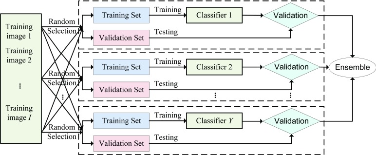
To boost the discriminative power of the above learned GSDs, we propose in this paper a novel learning scheme, namely, global discriminative dictionary learning. As shown in Fig. 3, this approach involves two novel strategies: (1) sparse dictionary learning with feature selection and (2) discriminative integration of representation residuals by LDA learning.

FIG. 3.

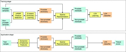
Diagram of discriminative dictionary learning framework. Each discriminative dictionary is in charge of tissue differentiation in a subsurface of prostate. Training a discriminative dictionary includes dictionary learning with mRMR feature selection followed by LDA learning.

2.B.1.b.1. Sparse dictionary learning with mRMR feature selection. In order to improve the discrimination between two learned subdictionaries (${\mathit{D}}_{\mathrm{PR}}\in {\mathbb{R}}^{M\times Q_{\mathrm{PR}}}$ and ${\mathit{D}}_{\mathrm{NPR}}\in {\mathbb{R}}^{M\times Q_{\mathrm{NPR}}}$), dictionary learning should be constrained in a discriminative feature space, so that each atom in different subdictionaries can be as distinctive as possible. In our study, we propose to combine feature selection with dictionary learning to learn the distinctive and compact subdictionaries ${\widehat{\mathbf{D}}}_{\mathrm{PR}}\in {\mathbb{R}}^{M^{\prime }\times {\widehat{Q}}_{\mathrm{PR}}}$ and ${\widehat{\mathbf{D}}}_{\mathrm{NPR}}\in {\mathbb{R}}^{M^{\prime }\times {\widehat{Q}}_{\mathrm{NPR}}}$, where M^′ ≪ M, ${\widehat{Q}}_{\mathrm{PR}}\ll Q_{\mathrm{PR}}$, and ${\widehat{Q}}_{\mathrm{NPR}}\ll Q_{\mathrm{NPR}}$.

First, the minimal redundancy maximal relevance algorithm³³ is employed to build a discriminative feature space. Compared to other feature selection methods³⁸ that only select individual features with the highest discrimination, mRMR minimizes the redundancy of the selected features as well. Thus, the selected features span a discriminative and compact subspace in which prostate and nonprostate tissues are well separated.

For each voxel, we first extract the 3D intensity patch centered at this voxel and then concatenate the patch as a column vector. This vector is used as the feature vector for each voxel. Assume that each sample is represented by the feature vector $\mathit{f}\in {\mathbb{R}}^M$; given Q training samples taken from both prostate and nonprostate regions, a feature matrix $\mathit{F}=\left[{\mathit{f}}^1,...,{\mathit{f}}^q,...,{\mathit{f}}^Q\right]$ is thus composed. f ^q(m), q = 1, …, Q, m = 1, …, M denotes the mth feature of the qth sample. The feature selection approach of mRMR aims to find a set of discriminative and compact features indexed by ${\mathit{P}}^{\mathrm{opt}}=\left\{p_{m^{\prime }}|m^{\prime }=1,...,M^{\prime },p_{m^{\prime }}\in \left\{1,...,M\right\}\right\}$ and then reduces feature vector ${\mathit{f}}^q$ of the qth training sample to ${\widehat{\mathbf{f}}}^q$, which contains only the features indexed by ${\mathit{P}}^{\mathrm{opt}}$. The criterion of the max-relevance and min-redundancy is formulated as follows:

$$\begin{array}{ccc}& & {\mathit{P}}^{\mathrm{opt}}=\arg {\max }_{\mathit{P}}\left({\Phi }_1-{\Phi }_2\right)\hfill \\ & & {\Phi }_1=\frac{1}{M^{\prime }}\sum _{p\in \mathit{P}}\mathrm{MI}\left({\mathit{F}}_p^{\mathrm{T}},\mathit{g}\right)\hfill \\ & & {\Phi }_2=\frac{1}{M^{\prime 2}}\sum _{p_a\in \mathit{P}}\sum _{p_b\in \mathit{P}}\mathrm{MI}\left({\mathit{F}}_{p_{\mathit{a}}}^{\mathrm{T}},{\mathit{F}}_{p_b}^{\mathrm{T}}\right),\hfill \end{array}$$ (7)

where Φ₁ measures the relevance of selected features to the class label (with, for example, class label “1” indicating a voxel belongs to the prostate region and class label “0” indicating a voxel belongs to a nonprostate region), Φ₂ measures the redundancy between selected features, M^′ is the number of selected features, ${\mathit{F}}_p\in {\mathbb{R}}^{1\times Q}$ returns the pth row of feature matrix F, $\mathit{g}\in {\mathbb{R}}^{Q\times 1}$ is the label vector of Q training samples, $\mathrm{MI}\left({\mathit{F}}_p^{\mathrm{T}},\mathit{g}\right)$ measures the mutual information between the pth feature and class label, and $\mathrm{MI}\left({\mathit{F}}_{p_{\mathit{a}}}^{\mathrm{T}},{\mathit{F}}_{p_b}^{\mathrm{T}}\right)$ measures the mutual information between the p_ath feature and the p_bth feature.

After mRMR feature selection, the feature vector $\mathit{f}\in {\mathbb{R}}^M$ of each training sample is now represented by a reduced feature vector $\widehat{\mathbf{f}}\in {\mathbb{R}}^{M^{\prime }}$, which includes only the set of selected features. Accordingly, we can obtain the respective subdictionaries for prostate and nonprostate classes, each including a set of dimensionality-reduced feature vectors, but with the same number of samples as the original subdictionary. Finally, we can further reduce the number of samples in each subdictionary and obtain the final subdictionaries ${\widehat{\mathbf{D}}}_{\mathrm{PR}}$ and ${\widehat{\mathbf{D}}}_{\mathrm{NPR}}$ as detailed below.

In our study, the K-means algorithm is employed to learn these two subdictionaries $\left\{{\mathit{D}}_{\mathrm{PR}},{\mathit{D}}_{\mathrm{NPR}}\right\}$. Different from standard dictionary learning,³⁷ which aims to optimally represent the training samples, the K-means algorithm learns a compact dictionary for better preserving the discriminability between training samples. Specifically, the K-means algorithm is applied to select Q_PR and Q_NPR clustering centroids from the respective prostate and nonprostate training samples as dictionary atoms. In contrast to most dictionary learning methods that often focus on sample representation and thus may produce similar subdictionaries with high correlation, K-means dictionary learning aims to preserve the discriminability obtained through feature selection while simultaneously reducing the number of dictionary atoms.

For now, since the dictionary learning is constrained in a discriminative space, the learned subdictionaries will contain discriminative information. Consequently, ${\widehat{\mathbf{D}}}_{\mathrm{PR}}\in {\mathbb{R}}^{M^{\prime }\times {\widehat{Q}}_{\mathrm{PR}}}$ and ${\widehat{\mathbf{D}}}_{\mathrm{NPR}}\in {\mathbb{R}}^{M^{\prime }\times {\widehat{Q}}_{\mathrm{NPR}}}$ encode distinctive appearance characteristics, which can be used to classify prostate and nonprostate tissues. By solving the sparse representation problem of Eq. (4) using the combined dictionary $\widehat{\mathbf{D}}=\left[{\widehat{\mathbf{D}}}_{\mathrm{PR}},{\widehat{\mathbf{D}}}_{\mathrm{NPR}}\right]$, the reconstruction residual $\widehat{\mathbf{r}}={\left[{\widehat{\mathbf{r}}}_{\mathrm{PR}}^{\mathrm{T}},{\widehat{\mathbf{r}}}_{\mathrm{NPR}}^{\mathrm{T}}\right]}^{\mathrm{T}}$ can be computed from the sparse coefficients ${\widehat{\mathbf{\alpha }}}_{\mathrm{PR}}$ and ${\widehat{\mathbf{\alpha }}}_{\mathrm{NPR}}$as below

$${\widehat{\mathbf{r}}}_{\mathrm{PR}}=\widehat{\mathbf{f}}-{\widehat{\mathbf{D}}}_{\mathrm{PR}}{\widehat{\mathbf{\alpha }}}_{\mathrm{PR}}{\widehat{\mathbf{r}}}_{\mathrm{NPR}}=\widehat{\mathbf{f}}-{\widehat{\mathbf{D}}}_{\mathrm{NPR}}{\widehat{\mathbf{\alpha }}}_{\mathrm{NPR}}.$$ (8)

2.B.1.b.2. Discriminative integration of representation residuals. After the reconstruction residuals are obtained by solving the sparse representation problem of Eqs. (4) and (8), we can directly compare the norms to derive the prostate likelihood as in standard dictionary learning (GSD). However, the residual elements from different features are not equally important. Features with more discriminative power are more likely to provide informative residuals than those with less discrimination. Therefore, we propose to learn the optimal weights by Fisher linear discriminative analysis (Fisher-LDA) for better utilization of reconstruction residuals for tissue separation.

Specifically, we learn a linear classifier in the residual space by Fisher-LDA. Thus, by combining the discriminative dictionary learning and Fisher-LDA residual integration, the external energy E_ext of our deformable model can be reformulated as below

$$\begin{array}{c}\hfill E_{\mathrm{ext}}=-{\sum }_i⟨{\overrightarrow{\nabla h}}_i,{\vec{\mathbf{n}}}_i⟩,h_i=\mathrm{sigmoid}\left({\mathit{\omega }}^{\mathrm{T}}\left(\begin{array}{c}{\widehat{\mathbf{r}}}_{\mathrm{PR}}\\ {\widehat{\mathbf{r}}}_{\mathrm{NPR}}\end{array}\right)-\delta \right),\end{array}$$ (9)

where sigmoid(·) denotes the sigmoid function. The parameters of the classifier, $\mathit{\omega }\in {\mathbb{R}}^{2M^{\prime }}$ and δ, are calculated as

$$\mathit{\omega }={\mathrm{argmax}}_{\mathit{\omega }}\frac{{\mathit{\omega }}^T{\mathit{\Gamma }}_{\mathrm{B}}\mathit{\omega }}{{\mathit{\omega }}^T{\mathit{\Gamma }}_{\mathrm{W}}\mathit{\omega }},\delta ={\mathit{\omega }}^T·\frac{{\mathit{\mu }}_{\mathrm{PR}}+{\mathit{\mu }}_{\mathrm{NPR}}}{2.0},$$ (10)

where ${\mathit{\Gamma }}_{\mathrm{B}}$ and ${\mathit{\Gamma }}_{\mathrm{W}}$ are the interclass and the intraclass scatter matrices in the residual space $\widehat{\mathbf{r}}$. ${\mathit{\mu }}_{\mathrm{PR}}$ and ${\mathit{\mu }}_{\mathrm{NPR}}$ denote average prostate residuals ${\widehat{\mathbf{r}}}_{\mathrm{PR}}$ and average nonprostate residuals ${\widehat{\mathbf{r}}}_{\mathrm{NPR}}$, respectively.

In Eq. (9), elements in the residual vectors $\left(\begin{array}{c}{\widehat{\mathbf{r}}}_{\mathrm{PR}}\\ {\widehat{\mathbf{r}}}_{\mathrm{NPR}}\end{array}\right)$ are assigned with different weights (by the corresponding elements in $\mathit{\omega }$) for optimally separating the prostate from nonprostate tissues, which further improves the discriminative power of standard dictionary learning.

II.B.1.C. Distributed discriminant dictionary (DDD) learning

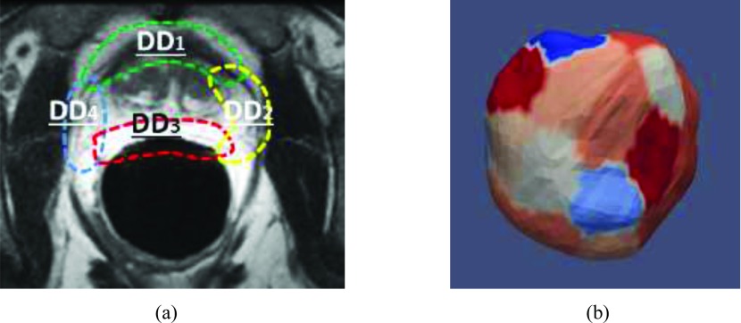
Based on the aforementioned strategies, GDD learning has been effectively exploited to separate the prostate from other tissues. However, this method still encounters challenges from large appearance variations along the prostate boundary [cf., Fig. 4(a)]. It is worth noting that the appearance variations within local regions are relatively small [such as the local regions indicated by different colors of dashed curves in Fig. 4(a)]. Based on this observation, we design a “divide-and-conquer” learning strategy, in which the global surface is partitioned into a set of subsurfaces with consistent appearance. Discriminant dictionary learning is applied on these distributed subsurfaces to further improve the performance of tissue differentiation.

FIG. 4.

Illustration of distributed dictionary learning. (a) Diagram of distributed dictionaries: A schematic explanation of distributed discriminative dictionaries, with each taking charge of tissue differentiation in a local region. (b) Surface parcellation: The partition of our deformable model, where different subsurfaces are indicated by different colors.

Specifically, the deformable model is divided into L subsurfaces corresponding to L local regions along the prostate boundary [cf., Fig. 4(b)]. This can be achieved using the vertex clustering method proposed in Ref. 32, which ensures the appearance variation around each subsurface is small. In this way, each subsurface l ∈ {1, …, L} can be attached by a pair of distributed subdictionaries, ${\widehat{\mathbf{D}}}_{\mathrm{PR}}^l$ and ${\widehat{\mathbf{D}}}_{\mathrm{NPR}}^l$, learned from samples extracted around the lth subsurface. Due to smaller appearance variation around each subsurface, these distributed dictionaries can better encode local appearance characteristics than the global dictionaries (such as GSD and GDD) and thus achieve more accurate tissue classification. It is worth noting that the learning process for each distributed subdictionary in DDD is the same as Fig. 3 except that it only targets to a local partition of the surface, instead of the entire surface as in GDD learning.

Based on the learned set of distributed subdictionaries, ${\widehat{\mathbf{D}}}_{\mathrm{PR}}^l$ and ${\widehat{\mathbf{D}}}_{\mathrm{NPR}}^l$, and sparse coefficients, ${\widehat{\mathbf{\alpha }}}_{\mathrm{PR}}^l$ and ${\widehat{\mathbf{\alpha }}}_{\mathrm{NPR}}^l$, the reconstruction residual ${\widehat{\mathbf{r}}}^l={[{\left({\widehat{\mathbf{r}}}_{\mathrm{PR}}^l\right)}^{\mathrm{T}},{\left({\widehat{\mathbf{r}}}_{\mathrm{NPR}}^l\right)}^{\mathrm{T}}]}^{\mathrm{T}}$ for a testing sample $\widehat{\mathbf{f}}$ can be computed by the mapping functions ${\widehat{\mathbf{r}}}_{\mathrm{PR}}^l=\widehat{\mathbf{f}}-{\widehat{\mathbf{D}}}_{\mathrm{PR}}^l{\widehat{\mathbf{\alpha }}}_{\mathrm{PR}}^l$ and ${\widehat{\mathbf{r}}}_{\mathrm{NPR}}^l=\widehat{\mathbf{f}}-{\widehat{\mathbf{D}}}_{\mathrm{NPR}}^l{\widehat{\mathbf{\alpha }}}_{\mathrm{NPR}}^l$. Thus, the external energy function E_ext can be further reformulated as

$$\begin{array}{ccc}& & E_{\mathrm{ext}}=-\sum _{l=1}^L\sum _{i\in {\mathcal{H}}_{\mathit{l}}}⟨{\overrightarrow{\nabla h}}_i^l,{\vec{\mathbf{n}}}_i⟩,\hfill \\ & & h_i^l=\mathrm{sigmoid}\left({\mathit{\omega }}^{l^{\mathrm{T}}}\left(\begin{array}{c}{\widehat{\mathbf{r}}}_{\mathrm{PR}}^l\\ {\widehat{\mathbf{r}}}_{\mathrm{NPR}}^l\end{array}\right)-{\delta }^l\right),\hfill \end{array}$$ (11)

where $h_i^l$ denotes the prostate likelihood of the ith vertex estimated by distributed dictionaries at the lth subsurface. This equation has the same form as in Eq. (9) but with different distributed dictionaries ${\widehat{\mathbf{D}}}_{\mathrm{PR}}^l$ and ${\widehat{\mathbf{D}}}_{\mathrm{NPR}}^l$. ${\mathcal{H}}_{\mathit{l}}$ is the index set for the vertices contained in the lth subsurface, and ${\vec{\mathbf{n}}}_i$ is the normal direction of the ith vertex on the deformable surface. These local tissue scores are used as appearance cues to guide subsurfaces onto the prostate boundary during deformable segmentation. For overlapping regions between two neighboring subsurfaces, the tissue scores are estimated by the minimum distance criteria: each voxel is labeled by the subsurface whose central point is the closest to the voxel.

II.B.1.D. Ensemble learning framework

According to the proposed distributed discriminative dictionary learning method, we can learn one dictionary for each subsurface. Due to the large number of voxels around each subsurface, typically we randomly select a subset of voxels to serve as training data. However, this approach may lead to a low-accuracy classifier if the sampled voxels are not representative. To relieve this phenomenon and increase the robustness of sparse representation-based classification, we use the idea of bagging³⁹ in our DDD learning. Specifically, for each subsurface, we learn a set of classifiers, instead of one. Each classifier is trained by randomly sampling voxels near the corresponding subsurface. To filter out those bad classifiers, we use tenfold cross validation. Specifically, each classifier is trained with 90% of the training MR images, and then its performance is tested on the remaining 10% of images. Only those classifiers with above-average performance are retained for the testing stage. Figure 5 shows the ensemble-classifier scheme of our learning method.

FIG. 5.

Ensemble-classifier scheme of dictionary learning. In the training stage, by further dividing the entire training sample dataset into training and validation sets, we can train Y classifiers by performing DDD learning and further test the performance of each.

Once multiple classifiers are learned per subsurface, we use averaging to combine the response from different classifiers. By integrating classification responses from the classifiers trained with different training samples, the robustness of final classification is improved.

II.B.2. Shape model

In Sec. II B 1, we propose to model the external energy E_ext in the deformable model by sparse learning techniques. In this way, the appearance model is built in a nonparametric fashion, which relieves the limitation of the Gaussian assumption in the ASM. Following the same idea, it is also important to build a nonparametric shape model. In deformable segmentation, the shape model is incorporated by iteratively minimizing the internal energy function E_int, which encodes the geometric characteristics of the model. This model is defined to prevent large irregular deformation and preserve the geometric properties of the organ. Specifically, E_int can be decomposed into two terms, E_shape and E_smooth, as shown in Eq. (12),

$$E_{\mathrm{int}}=E_{\mathrm{shape}}+{\lambda }_1{E}_{\mathrm{smooth}}.$$ (12)

The first term E_shape constrains the deformable model in a learned shape subspace. The second term E_smooth ensures the smoothness of the surface in order to prevent large discrepancies between neighboring vertices.

In the shape term E_shape, we do not assume that the shape variation of prostates follows the Gaussian distribution, which is reasonable due to the large interpatient variability. Thus, instead of using PCA for shape modeling as in Eq. (3), we use a recently proposed method called sparse shape composition method⁴⁰ to model the shape prior. Specifically, by denoting ${\mathit{D}}_{\mathrm{s}}$ as a large shape repository that includes the shape instances of training subjects, the approximation of an input shape vector v by ${\mathit{D}}_{\mathrm{s}}$ is formulated as the following optimization problem in the SSC method:

$$\begin{array}{ccc}\hfill \left({\mathit{\alpha }}_{\mathrm{s}}^{\mathrm{opt}},{\psi }^{\mathrm{opt}},{\mathit{e}}^{\mathrm{opt}}\right)& =& {\mathrm{argmin}}_{{\mathit{\alpha }}_{\mathrm{s}},\psi ,\mathit{e}}\Vert \psi \left(\mathit{v}\right)\hfill \\ & & -{\mathit{D}}_{\mathrm{s}}{\mathit{\alpha }}_{\mathrm{s}}{-\mathit{e}\Vert }^2+{\beta }_1\Vert {\mathit{\alpha }}_{\mathrm{s}}{\Vert }_1+{\beta }_2{\Vert \mathit{e}\Vert }_1.\hfill \end{array}$$ (13)

Here, ψ is an affine transformation matrix, which aligns surface vector v to the mean shape vector. ${\mathit{\alpha }}_{\mathrm{s}}$ denotes the sparsity coefficient for linear combination, and e compensates the large residual errors caused by a few mispositioned vertices. Here, we set β₂ = 0 during shape deformation, since we do not expect to compensate for irregular large deformations of few vertices. Minimization of Eq. (13) is a two-step iteration scheme. At each iteration, the affine transformation ψ is first estimated. Then, based on the current estimated ψ, Eq. (13) can be solved as a sparse representation problem. These two steps are iteratively performed until convergence.

With the help of SSC, we can easily represent the current surface vector v by inverse affine transformation of its sparse linear representation ${\psi }^{{\mathrm{opt}}^{-1}}\left({\mathit{D}}_{\mathrm{s}}{\mathit{\alpha }}_{\mathrm{s}}^{\mathrm{opt}}\right)$. So the shape prior for the shape regularization can be formulated as the shape internal energy below:

$$E_{\mathrm{shape}}=\Vert \mathit{v}-{\psi }^{{\mathrm{opt}}^{-1}}\left({\mathit{D}}_{\mathrm{s}}{\mathit{\alpha }}_{\mathrm{s}}^{\mathrm{opt}}\right){\Vert }_2^2.$$ (14)

Apart from the shape prior, the smooth constraint E_smooth is further used to prevent large deviations between neighboring vertices

$$E_{\mathrm{smooth}}=\sum _i{‖{\mathit{v}}_i-\frac{{\sum }_{{\mathbb{N}}_i}{\mathit{v}}_j}{{\sum }_{{\mathbb{N}}_i}1}‖}_2^2,$$ (15)

where ${\mathbb{N}}_i$ denotes the vertex set in the neighborhood with a certain radius around the vertex ${\mathit{v}}_i$.

By combining Eqs. (14) and (15) into Eq. (12), the internal forces at all vertices can be defined to ensure the nonparametric shape prior as well as the smoothness of the deformable model.

II.B.3. Summary

According to Secs. II B 1 and II B 2, we can construct both an appearance model (with external energy E_ext) and a shape model (with internal energy E_int) for deformable segmentation. In the application stage, the surface model is deformed to locate the prostate boundary by minimizing energy E defined in Eq. (1). Specifically, the model deforms to fit the appearance cues provided by DDD [Eq. (11)] and is also constrained by a SSC-based shape prior [Eq. (14)]. In this subsection, we summarize our proposed deformable segmentation algorithm by giving more details to the initialization and optimization of the deformable model.

II.B.3.A. Initialization strategy

Quickly and accurately locating the position of the prostate in subject space is crucial for deformable model segmentation.⁴¹ One simple solution is to first detect the key landmarks on the subject image. Then, a similarity transformation can be found between the detected landmarks and the corresponding ones in the mean shape. Finally, the mean shape can be accordingly warped onto the subject space for initialization. However, the mean shape may be not a good initialization due to large prostate shape variations across subjects. Therefore, we employ a sparse shape composition to infer a shape from the SSC shape space using the detected landmarks. First, seven landmarks (which are located at the central, left, right, base, apex, anterior, and posterior of the prostate) are detected on the prostate image using a learning-based method.⁴² Then, a sparse shape composition method is used to infer an initial shape based on the matching of detected landmarks. Specifically, by solving Eq. (13), a sparse code is computed based on the seven detected landmarks and their corresponding landmarks on the training shapes. Particularly, for surface model initialization, we set β₂ = 1 for Eq. (13) to compensate the potential misdetected landmarks. Then, the obtained sparse codes are applied to the corresponding training shapes to derive a refined shape. Finally, the initial deformable model is obtained by transforming the refined shape back to the subject image space.

II.B.3.B. Optimization strategy

Our deformable segmentation algorithm via distributed discriminative dictionary and ensemble learning is summarized in Algorithm 1:

Deformable Segmentation Algorithm via Distributed Discriminative Dictionary and Ensemble Learning.

Input: Testing image ${\mathit{A}}_0$

Output: Segmented binary image ${\mathit{B}}_0$

Initialization: t = 0

Estimate the initial shape parameter $({\mathit{\alpha }}_{\mathrm{s}}^0,{\psi }^0,{\mathit{e}}^0)$ and obtain the initial deformable surface ${\mathit{v}}^0$ by solving sparse learning problem in Eq. (13) with β1 = 5 and β2 = 1.

while 1 ⩽ t ⩽ T and $\Vert {\mathit{v}}^t-{\mathit{v}}^{t-1}{\Vert }_2^2>0.001$ do

“M” Step:

Evolve the deformable model ${\mathit{v}}^t$ by minimizing the external energyfunction Eext [Eq. (11)] and the smoothness internal energy functionEsmooth [Eq. (15)];

“E” Step:

a. Estimate the parameters $\left({\mathit{\alpha }}_{\mathrm{s}}^t,{\psi }^t\right)$ for the shape refinement bysolving optimization problem [Eq. (13)] with β1 = 5 and β2 = 0;

b. Refine the deformed shape ${\mathit{v}}^t$ by minimizing the shape internalenergy function [Eq. (14)] based on the computed parameters$\left({\alpha }_{\mathrm{s}}^t,{\psi }^t\right)$.

t = t + 1

end while

Convert the output shape ${\mathit{v}}^T$ to a binary image ${\mathit{B}}_0$

Return: Segmented binary image ${\mathit{B}}_0$

To optimize Eq. (1) for the deformable model, the expectation-maximization (EM) algorithm is applied to minimize both the external energy [Eq. (11)] and the internal energy [Eq. (12)] iteratively. The initial values of parameters $\left({\mathit{\alpha }}_{\mathrm{s}}^{\mathrm{opt}},{\psi }^{\mathrm{opt}},{\mathit{e}}^{\mathrm{opt}}\right)$ for building the initial shape ${\mathit{v}}^0$ are first estimated as $\left({\mathit{\alpha }}_{\mathrm{s}}^0,{\psi }^0,{\mathit{e}}^0\right)$ by solving the sparse coding problem of Eq. (13). Then, the “M” step and “E” step are alternately carried out until convergence. First, in the “M” step, the external energy and smooth internal energy are used to guide the deformable model toward the prostate boundary. During deformation, each vertex of the deformable model is updated via a local search along its normal direction on the deformable model. That means the vertex location on the deformed surface is mainly updated according to the appearance information. Second, in the “E” step, the parameters $\left({\mathit{\alpha }}_{\mathrm{s}}^t,{\psi }^t\right)$ in the tth iteration are estimated by finding a closest shape in the SSC-based shape space to the current deformed shape. Then, the deformed shape is refined using the estimated parameters $\left({\mathit{\alpha }}_{\mathrm{s}}^t,{\psi }^t\right)$. In this step, high-level shape information is employed to constrain and regularize the deformed shape. Therefore, the possibility of getting stuck in local minima is reduced in the deformable segmentation. In this EM optimization framework, the surface will iteratively deform to the prostate boundary while preserving the shape characteristics of the prostate.

III. EXPERIMENTS

III.A. Materials and parameter settings

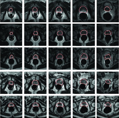
Our method was evaluated on both internal and public datasets. The internal dataset contains 75 T2-weighted MR images with ground truth segmentations provided by a clinical expert. These images were acquired from the University of Chicago Hospital and scanned from different patients with different MRI scanners. As shown in Fig. 6, this dataset includes large variations on both appearances and shapes. In addition, the dimension and spacing are not constant for all 3D images. The image dimension varies from 256 × 256 × 28 to 512 × 512 × 30, and the image spacing varies from 0.49 × 0.49 × 3 to 0.56 × 0.56 × 5 mm. For the public dataset, we used the MICCAI 2012 challenge data, which contains 50 T2-weighted MR images with corresponding ground truth segmentations. In our application, histogram matching is used to normalize the global histograms across different images as a preprocessing step. In our study, positive samples are the voxels inside the prostate, and negative samples are the voxels outside the prostate. Each voxel is represented by the image features extracted from the local patch centered at that voxel. During the training stage, we randomly extract voxels near the prostate boundary as training voxels. To avoid the imbalance in classification, we extract the same number of positive and negative samples according to the manually segmented prostate for each training image.

FIG. 6.

Five typical examples of T2-weighted MR prostate images. Due to the existence of partial volume effects and interpatient differences, there are large variations on both prostate appearance and shape in the dataset.

In terms of parameter settings of the algorithm, the triangle mesh is composed of 2215 vertices and 4306 polygons in the deformable model. The number of classifiers in the ensemble learning is set as 10. Our algorithm was implemented in MATLAB. The typical computational time for segmenting a prostate is 1–2 min with parallel computing. We expect to further improve the efficiency of our algorithm by implementing it in C++.

III.B. Evaluation criteria

For quantitative evaluations, the Dice similarity coefficient (DSC), sensitivity, positive predictive value (PPV), and average surface distance (ASD) are employed.⁴³ DSC, sensitivity, and PPV are used as metrics to evaluate the spatial overlap agreement between manual segmentation and automated segmentation, in which higher values indicate more accurate segmentations. ASD is a surface-based performance measure calculated as the average distance between the manually segmented shape and the automatically segmented shape. Lower values of ASD reflect more accurate segmentations. The following gives the formulas for the above four measurements:

$$\begin{array}{c}\hfill \begin{array}{c}\mathrm{DSC}=\frac{2\mathrm{TP}}{2\mathrm{TP}+\mathrm{FP}+\mathrm{FN}},\mathrm{Sensitivity}=\frac{\mathrm{TP}}{\mathrm{TP}+\mathrm{FN}},\mathrm{PPV}=\frac{\mathrm{TP}}{\mathrm{TP}+\mathrm{FP}}\hfill \\ \mathrm{ASD}=\frac{1}{2}\left(\frac{{\sum }_{{\mathit{v}}_i\in {\mathit{v}}_{\mathrm{SEG}}}d\left({\mathit{v}}_i,{\mathit{v}}_{\mathrm{MAN}}\right)}{{\sum }_{{\mathit{v}}_i\in {\mathit{v}}_{\mathrm{SEG}}}1}+\frac{{\sum }_{{\mathit{v}}_i\in {\mathit{v}}_{\mathrm{MAN}}}d\left({\mathit{v}}_i,{\mathit{v}}_{\mathrm{SEG}}\right)}{{\sum }_{{\mathit{v}}_i\in {\mathit{v}}_{\mathrm{MAN}}}1}\right)\hfill \end{array},\end{array}$$ (16)

where TP, FP, and FN are the number of true positives, false positives, and false negatives, respectively. $d\left({\mathit{v}}_i,{\mathit{v}}_{\mathrm{MAN}}\right)$ is the minimum distance between vertex ${\mathit{v}}_i$ of the automatically segmented prostate surface ${\mathit{v}}_{\mathrm{SEG}}$ (${\mathit{v}}_i\in {\mathit{v}}_{\mathrm{SEG}}$) to the vertices of the manually segmented shape ${\mathit{v}}_{\mathrm{MAN}}$. Similarly, $d\left({\mathit{v}}_i,{\mathit{v}}_{\mathrm{SEG}}\right)$ is the minimum distance between vertex ${\mathit{v}}_i$ of the manually segmented shape ${\mathit{v}}_{\mathrm{MAN}}$ (${\mathit{v}}_i\in {\mathit{v}}_{\mathrm{MAN}}$) to the vertices of the segmented prostate surface ${\mathit{v}}_{\mathrm{SEG}}$. ${\sum }_{{\mathit{v}}_i\in {\mathit{v}}_{\mathrm{SEG}}}1$ and ${\sum }_{{\mathit{v}}_i\in {\mathit{v}}_{\mathrm{MAN}}}1$ denote the number of vertices on surfaces ${\mathit{v}}_{\mathrm{SEG}}$ and ${\mathit{v}}_{\mathrm{MAN}}$, respectively.

In our experiments, we validate our method by k-fold cross validation. Specifically, the entire dataset is divided into k folds. For each round of evaluation, onefold is used as testing data and the other k-1 folds are used as training data. Specifically, threefold cross validation is used for the internal dataset and fivefold cross validation is adopted for the MICCAI challenge dataset. For each round of training, if not explicitly mentioned, ten global/local classifiers are constructed by randomly selecting 90% of the training images as training data and using the rest as validation images to measure the classification performance.

III.C. Experimental results on internal database

III.C.1. Evaluation on the proposed four variants of dictionary learning methods

We first evaluate the tissue classification performance of the proposed four variants of dictionary learning methods: GSD learning, GDD learning, DSD, and DDD learning.

• •GSD: a pair of global dictionaries learned by the standard dictionary learning method;
• •GDD: a pair of global dictionaries learned by the proposed discriminative dictionary learning method;
• •DSD: a set of distributed dictionaries learned by the standard dictionary learning method.
• •DDD: a set of distributed dictionaries learned by the proposed discriminative dictionary learning method.

In this experiment, we evaluate each component of our method separately in order to demonstrate the effectiveness of our proposed DDD learning approach. To exclude the influence from ensemble learning, we train only one classifier at each subsurface for DSD and DDD, and one global classifier for GSD and GDD.

A visual comparison of the classification results produced by the above four dictionary learning methods is demonstrated in Fig. 7. Figure 7(a) shows a slice of an original T2-weighted image with the contour indicating the ground-truth prostate boundary manually delineated by clinician. Figures 7(b)–7(e) demonstrate the corresponding classification results from the GSD, GDD, DSD, and DDD learning methods, respectively. Comparing (b) and (c), we can see that the rate of misclassification is largely reduced when discriminative dictionary learning is used. However, there are still classification errors, especially in the local prostate regions (i.e., anterior) that have similar appearance with neighboring tissues. In this case, the distributed dictionary can be adopted to further improve the classification result, since each classifier is only targeting to a local prostate region and is thus more specific than a global classifier. By combining both distributed classifiers and discriminative dictionary learning, we finally obtain the best classification result using DDD learning, as shown in Fig. 7(e).

FIG. 7.

A typical slice of a T2-weighted MR image with manual segmentation (a) and its classification results by four dictionary-learning methods, GSD (b), GDD (c), DSD (d), and DDD (e), respectively.

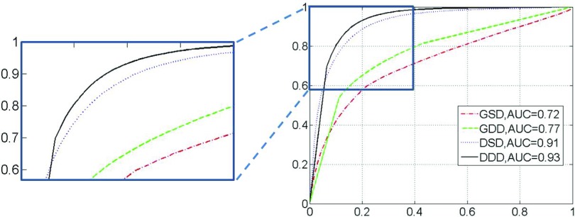
To quantitatively compare the four different dictionary learning methods, the ROC curves and corresponding area under curve (AUC) for each approach are shown in Fig. 8. Just as the performance demonstrated in Fig. 7, DDD achieves the best tissue classification accuracy with an AUC of 0.93, while the AUCs of GSD, GDD, and DSD are 0.72, 0.77, and 0.91, respectively. It is worth noting that these four methods are different only in the “discriminative” and “distributed” learning strategies, which shows the efficacy of our proposed strategies in accurate tissue classification.

FIG. 8.

ROC curves of tissue classification using four different dictionary-learning methods. (Right) the complete ROC curves; (Left) A zoomed-in figure to show the top part of the ROC, which is indicated by the small rectangle.

III.C.2. Evaluation on the ensemble learning

In this section, we will evaluate the contribution of the ensemble learning framework for the above four dictionary learning methods.

Figure 9 shows the corresponding classification results of Fig. 7(a) by combing the GSD, GDD, DSD, and DDD with ensemble learning. We observe that our methods show some improvement on classification results when ensemble learning is incorporated.

FIG. 9.

Classification results produced by four dictionary-learning methods with ensemble learning. (a) GSD. (b) GDD. (c) DSD. (d) DDD.

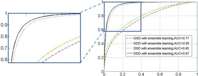
Similarly, the ROC curves of GSD, GDD, DSD, and DDD with ensemble learning are presented in Fig. 10. Comparing Fig. 10 with Fig. 8, we observe that the average increase in AUC for the four methods is more than 4%, which supports the notion that ensemble learning boosts the performance of all dictionary learning methods. It is worth noting that our proposed DDD learning approach still achieves the best performance in the ensemble learning framework.

FIG. 10.

ROC curves of tissue classification by integrating four different learning methods with ensemble learning. (Right) the complete ROC curves; (Left) A zoomed-in figure to show the top part of the ROC as indicated by the small rectangle.

III.C.3. Evaluation on the deformable prostate segmentation via DDD and ensemble learning

We further evaluated the segmentation accuracy of our deformable model via DDD and ensemble learning. Figure 11 shows the DSC, sensitivity, PPV and ASD measures of our proposed deformable model method on the 75 T2-weighted MR images. For 86% of images, our method obtains a DSC higher than 0.85 (with an average DSC of 0.89). Of all the 75 images, only one has a DSC value below 0.8. These results demonstrate the accuracy and robustness of our method in prostate segmentation. Figure 12 shows the box and whisker diagram of DSC, sensitivity, PPV, and ASD measures of our proposed deformable model method on all 75 images. The bottom and top of each box are the 25th and 75th percentiles, and the band near the middle is the 50th percentile. According to the distributions of these four measurements, our prostate segmentation method achieves a median DSC of 89.6%, a median Sensitivity of 92.8%, a median PPV of 90.0%, and a median ASD of 1.56 mm.

FIG. 11.

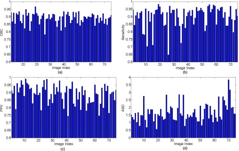
Diagrams of DSC (a), sensitivity (b), PPV (c), and ASD (d) measures of our proposed deformable model on all 75 T2-weighted MR images.

FIG. 12.

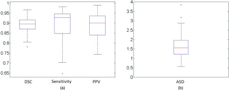
The box and whisker diagram of (a) DSC, sensitivity, PPV, and (b) ASD measures of our proposed deformable model for all 75 images.

To validate the performance of our method on segmenting the different zones of the prostate, we show the segmentation results of the apex, base, and central slices in Fig. 13, with a comparison to segmentation via the ASM method. As we can see, even though the appearance and shape is much more complicated on the base and apex regions than in the central region, our method still achieves accurate classification results. The average DSC of our segmentation method for the apex, central, and base regions of the prostate is 84.9%, 93.6%, and 81.8%, respectively, compared to 59.2%, 83.3%, and 58.7% obtained by the ASM method. Figure 14 shows the box and whisker diagrams of DSC on the apex, central, and base regions of the prostate by ASM and our proposed deformable model on all 75 images. According to the distributions of these three measurements, our prostate segmentation method achieves a median DSC of 86.7%, 94.2%, and 84.2% on the apex, central, and base regions of the prostate, respectively, which are much higher than the median scores obtained by the ASM method (67.5%, 86.6%, and 65.5%, respectively).

FIG. 13.

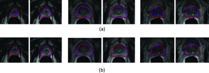
Typical segmentation results for prostate apex (left), central (middle), and base (right) regions of two patients produced by (a) ASM and (b) our proposed deformable model. The first row demonstrates the segmentation results for ASM, and the second row demonstrates the segmentation results for our proposed deformable model. The three main columns show the segmentation results for the apex, central, and base regions of the two patients, respectively. Light grey contours indicate the manual segmentations, and dark grey contours indicate the automatic segmentations.

FIG. 14.

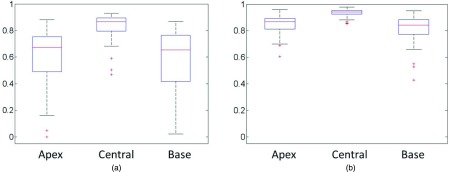
The box and whisker diagrams of DSC, measured at the apex, central, and base regions of the prostate, by (a) ASM and (b) our proposed deformable model for all 75 images.

To demonstrate the effectiveness of our deformable model in T2-weighted MR prostate segmentation, three other state-of-the-art prostate segmentation methods are compared with our method, including ASM and two multiatlas-based methods.^20,21 We adopt the best quantitative results reported in these works for our comparison. Table I reports the means and standard deviations of DSC, sensitivity, PPV, and ASD between automatic segmentations and manual segmentations for our method and the three other methods. It should be noted that our 75 images include 30 images used in Liao's method²¹ and 66 images used in Ref. 20. According to Table I, our method achieves the best performance among all methods under comparison. Figure 15 gives several visual segmentation results achieved by our method. It can be seen that despite the large variation of prostate appearance and shape, our method can still achieve accurate segmentation results.

TABLE I.

Mean values and standard deviations (Std) of DSC, sensitivity, PPV, and ASD between automatic segmentations and manual segmentations for our proposed method and three other methods on the internal dataset. NA in the table means the corresponding measurement was not reported in the literature. The best performance of each measurement is shown in bold lettering.

Method	Image No.	DSC (in%)	Sensitivity (in%)	PPV (in%)	ASD (in mm)
ASM	75	74.5 ± 11.3	75.7 ± 18.3	79.1 ± 11.8	4.16 ± 3.64
Liao et al. (Ref. 21)	30	86.7 ± 2.2	NA	NA	1.90 ± 1.60
Liao et al. (Ref. 20)	66	88.3 ± 2.6	NA	NA	1.8 ± 0.9
Our method	75	89.1 ± 3.6	89.9 ± 7.0	89.0 ± 6.2	1.67 ± 0.61

FIG. 15.

Typical segmentation results by our proposed deformable model. Each row shows the prostate of one subject automatically segmented by our method (white) and manually delineated by an expert (grey). Different columns indicate different transversal slices from the apex (left) to the base (right) of the prostate.

III.D. Experimental results on public database

We further evaluate our deformable model with DDD learning on the public MICCAI 2012 challenge database. Comparing with four other state-of-the-art prostate segmentation methods,^23,26,27,44 Table II reports the means and standard deviations of DSC, sensitivity, PPV, and ASD between automatic segmentations and manual segmentations for our method. Since all mentioned methods in Table II were evaluated on the same dataset, the comparisons are informative to show that our method achieves the best performance among all methods under comparison.

TABLE II.

Mean values and standard deviations (Std) of DSC, sensitivity, PPV, and ASD between automatic segmentations and manual segmentations for our proposed method and four other methods on the public dataset. NA in the table means the corresponding measurement was not reported in the literature. The best performance of each measurement is shown in bold lettering.

Method	Image No.	DSC (in%)	Sensitivity (in%)	PPV (in%)	ASD (in mm)
PASM (Ref. 26)	50	77.0 ± 23.0	NA	NA	4.10 ± 7.81
AAM (Ref. 27)	50	81.0 ± 12.0	NA	NA	NA
Martin et al. (Ref. 23)	50	84.0 ± NA	87.0 ± NA	84.0 ± NA	2.41 ± NA
Birkbeck et al. (Ref. 44)	50	86.0 ± NA	NA	NA	1.91 ± NA
Our method	50	87.4 ± 3.8	82.6 ± 7.2	93.3 ± 3.5	1.92 ± 0.90

IV. DISCUSSION

In our work, we learn a linear LDA classifier on sparse representation residuals for tissue classification. Another option is to learn a nonlinear classifier directly on the sparse representation. However, since sparse codes (i.e., sparse representations) are unstable, similar patches can have distinct sparse codes, which can limit the performance of nonlinear classifiers that are trained with sparse codes.⁴⁵

After applying the learned appearance model for voxelwise classification of the new image, we can obtain a prostate likelihood map, which is used for guiding deformable segmentation by finding the boundary voxels with the largest oriented gradient magnitude. The traditional deformable models (e.g., ASM and AAM), often use line profiles, which are just MR intensities. Therefore, these methods could be sensitive to MR inhomogeneity. Because we use an appearance model to map the original MR image into the prostate likelihood map, our deformable model largely avoids such a limitation.

Compared with other learning-based methods, our dictionary learning method has three main advantages. First, the dictionary learning method is nonparametric and can be used for nonlinear classification. This aspect is important for dealing with large interpatient appearance variations found in prostate MR images. Second, our approach requires less training time than other learning-based methods. In the training stage, the dictionaries are built by clustering the selected training samples. No complicated learning procedure is required, which makes the proposed method very easy to use and implement for other similar applications. Third, the dictionary learning method can also easily be extended to other multiclass classification problems.

Regarding the clinical application of our method, the resulting prostate segmentation is able to provide an accurate localization of the gland, which is required in many treatments for prostate cancer. For example, radiation therapy can thus be targeted to the prostate region with high precision, in order to reduce the risk of radiation exposure to the surrounding normal tissues. Additionally, estimating the prostate volume based on the segmentation result can also reduce the clinician's manual work by helping to automatically evaluate the treatment response.

However, our method still has some limitations, and many improvements could be envisioned. First, instead of separating the steps of feature selection and dictionary learning, we can combine them for joint discriminative dictionary learning to further boost the discriminative power of our method. Second, similar to the local appearance model, the shape model can also be built based on the local subsurfaces of the model. In this way, a sparse shape prior based on each local subsurface with small shape variation can better preserve the local shape details. Finally, a hierarchical deformable segmentation framework can also be adopted for improving the robustness and accuracy of the segmentation.

V. CONCLUSION

In this paper, we have presented a novel method to segment the prostate in MR images. To address the challenges presented by complicated appearances of the prostate, we designed a novel (DDD learning method to extract appearance characteristics in a nonparametric, discriminative, and local fashion. This approach was further integrated within an ensemble learning framework. A deformable model guided by the learned dictionaries and sparse shape prior was then developed to segment the prostate in T2-weighted MR images. Experimental results show that the proposed method has superior discriminant power on classification and consequently achieves the most accurate results compared to other state-of-the-art methods.

REFERENCES

- 1.Shukla-Dave A. and Hricak H., “Role of MRI in prostate cancer detection,” NMR Biomed. 27, 16–24 (2013). 10.1002/nbm.2934 [DOI] [PubMed] [Google Scholar]
- 2.Seifabadi R.et al. , “Accuracy study of a robotic system for MRI-guided prostate needle placement,” Int. J. Med. Rob. Comput. Assist. Surg. 9, 305–316 (2012). 10.1002/rcs.1440 [DOI] [PMC free article] [PubMed] [Google Scholar]
- 3.Blumenfeld P.et al. , “Transperineal prostate biopsy under magnetic resonance image guidance: A needle placement accuracy study,” J. Magn. Reson. Imaging 26, 688–694 (2007). 10.1002/jmri.21067 [DOI] [PubMed] [Google Scholar]
- 4.Zhan Y.et al. , “Registering histologic and MR images of prostate for image-based cancer detection,” Acad. Radiol. 14, 1367–1381 (2007). 10.1016/j.acra.2007.07.018 [DOI] [PMC free article] [PubMed] [Google Scholar]
- 5.Fedorov A.et al. , “Image registration for targeted MRI-guided transperineal prostate biopsy,” J. Magn. Reson. Imaging 36, 987–992 (2012). 10.1002/jmri.23688 [DOI] [PMC free article] [PubMed] [Google Scholar]
- 6.Shen D.et al. , “Optimized prostate biopsy via a statistical atlas of cancer spatial distribution,” Med. Image Anal. 8, 139–150 (2004). 10.1016/j.media.2003.11.002 [DOI] [PubMed] [Google Scholar]
- 7.Hricak H.et al. , “Imaging prostate cancer: A multidisciplinary perspective,” Radiology 243, 28–53 (2007). 10.1148/radiol.2431030580 [DOI] [PubMed] [Google Scholar]
- 8.Toth R.et al. , “Accurate prostate volume estimation using multifeature active shape models on T2-weighted MRI,” Acad. Radiol. 18, 745–754 (2011). 10.1016/j.acra.2011.01.016 [DOI] [PubMed] [Google Scholar]
- 9.Zhan Y. and Shen D., “Automated segmentation of 3D US prostate images using statistical texture-based matching method,” in Medical Image Computing and Computer-Assisted Intervention – MICCAI 2003, edited by Ellis R. and Peters T. (Springer, Berlin Heidelberg, 2003), Vol. 2878, pp. 688–696. [Google Scholar]
- 10.Zhu Y., Williams S., and Zwiggelaar R., “Computer technology in detection and staging of prostate carcinoma: A review,” Med. Image Anal. 10, 178–199 (2006). 10.1016/j.media.2005.06.003 [DOI] [PubMed] [Google Scholar]
- 11.Toth R. and Madabhushi A., “Multifeature landmark-free active appearance models: Application to prostate MRI segmentation,” IEEE Trans. Med. Imaging 31, 1638–1650 (2012). 10.1109/TMI.2012.2201498 [DOI] [PubMed] [Google Scholar]
- 12.Klein S.et al. , “Automatic segmentation of the prostate in 3D MR images by atlas matching using localized mutual information,” Med. Phys. 35, 1407–1417 (2008). 10.1118/1.2842076 [DOI] [PubMed] [Google Scholar]
- 13.Sabuncu M. R.et al. , “A generative model for image segmentation based on label fusion,” IEEE Trans. Med. Imaging 29, 1714–1729 (2010). 10.1109/TMI.2010.2050897 [DOI] [PMC free article] [PubMed] [Google Scholar]
- 14.Warfield S. K., Zou K. H., and Wells W. M., “Simultaneous truth and performance level estimation (STAPLE): An algorithm for the validation of image segmentation,” IEEE Trans. Med. Imaging 23, 903–921 (2004). 10.1109/TMI.2004.828354 [DOI] [PMC free article] [PubMed] [Google Scholar]
- 15.Coupé P.et al. , “Patch-based segmentation using expert priors: Application to hippocampus and ventricle segmentation,” NeuroImage 54, 940–954 (2011). 10.1016/j.neuroimage.2010.09.018 [DOI] [PubMed] [Google Scholar]
- 16.Wang H.et al. , “Optimal weights for multi-atlas label fusion,” in Information Processing in Medical Imaging, edited by Székely G. and Hahn H. (Springer, Berlin Heidelberg, 2011), Vol. 6801, pp. 73–84. [DOI] [PMC free article] [PubMed] [Google Scholar]
- 17.Rousseau F., Habas P. A., and Studholme C., “A supervised patch-based approach for human brain labeling,” IEEE Trans. Med. Imaging 30, 1852–1862 (2011). 10.1109/TMI.2011.2156806 [DOI] [PMC free article] [PubMed] [Google Scholar]
- 18.Asman A. and Landman B., “Characterizing spatially varying performance to improve multi-atlas multi-label segmentation,” in Information Processing in Medical Imaging, edited by Székely G. and Hahn H. (Springer, Berlin Heidelberg, 2011), Vol. 6801, pp. 85–96. [DOI] [PMC free article] [PubMed] [Google Scholar]
- 19.Langerak T. R.et al. , “Label fusion in atlas-based segmentation using a selective and iterative method for performance level estimation (SIMPLE),” IEEE Trans. Med. Imaging 29, 2000–2008 (2010). 10.1109/TMI.2010.2057442 [DOI] [PubMed] [Google Scholar]
- 20.Liao S.et al. , “Automatic prostate MR image segmentation with sparse label propagation and domain-specific manifold regularization,” in Information Processing in Medical Imaging, edited by Gee J.et al. (Springer, Berlin Heidelberg, 2013), Vol. 7917, pp. 511–523. [DOI] [PMC free article] [PubMed] [Google Scholar]
- 21.Liao S.et al. , “Representation learning: A unified deep learning framework for automatic prostate MR segmentation,” in Medical Image Computing and Computer-Assisted Intervention – MICCAI 2013, edited by Mori K.et al. (Springer, Berlin Heidelberg, 2013), Vol. 8150, pp. 254–261. [DOI] [PMC free article] [PubMed] [Google Scholar]
- 22.Tsai A.et al. , “A shape-based approach to the segmentation of medical imagery using level sets,” IEEE Trans. Med. Imaging 22, 137–154 (2003). 10.1109/TMI.2002.808355 [DOI] [PubMed] [Google Scholar]
- 23.Martin S., Troccaz J., and Daanen V., “Automated segmentation of the prostate in 3D MR images using a probabilistic atlas and a spatially constrained deformable model,” Med. Phys. 37, 1579–1590 (2010). 10.1118/1.3315367 [DOI] [PubMed] [Google Scholar]
- 24.Toth R.et al. , “A magnetic resonance spectroscopy driven initialization scheme for active shape model based prostate segmentation,” Med. Image Anal. 15, 214–225 (2011). 10.1016/j.media.2010.09.002 [DOI] [PMC free article] [PubMed] [Google Scholar]
- 25.Zhan Y. and Shen D., “Deformable segmentation of 3-D ultrasound prostate images using statistical texture matching method,” IEEE Trans. Med. Imaging 25, 256–272 (2006). 10.1109/TMI.2005.862744 [DOI] [PubMed] [Google Scholar]
- 26.Kirschner M., Jung F., and Wesarg S., “Automatic prostate segmentation in MR images with a probabilistic active shape model,” Paper presented at the PRostate MR Image SEgmentation, PROMISE 2012 (Nice, France, 2012). [Google Scholar]
- 27.Maan B. and Heijden F. v. d., “Prostate MR image segmentation using 3D active appearance models,” Paper presented at the PRostate MR Image SEgmentation, PROMISE 2012 (Nice, France, 2012). [Google Scholar]
- 28.Wright J.et al. , “Robust face recognition via sparse representation,” IEEE Trans. Pattern Anal. Mach. Intell. 31, 210–227 (2009). 10.1109/TPAMI.2008.79 [DOI] [PubMed] [Google Scholar]
- 29.Mairal J.et al. , “Non-local sparse models for image restoration,” in Proceedings of the IEEE 12th International Conference on Computer Vision, 2009 (IEEE, Piscataway, NJ, 2009), pp. 2272–2279. [Google Scholar]
- 30.Wright J.et al. , “Sparse representation for computer vision and pattern recognition,” Proc. IEEE 98, 1031–1044 (2010). 10.1109/JPROC.2010.2044470 [DOI] [Google Scholar]
- 31.Candès E., Wakin M., and Boyd S., “Enhancing sparsity by reweighted ℓ1 minimization,” J. Fourier Anal. Appl. 14, 877–905 (2008). 10.1007/s00041-008-9045-x [DOI] [Google Scholar]
- 32.Zhang S., Zhan Y., and Metaxas D. N., “Deformable segmentation via sparse representation and dictionary learning,” Med. Image Anal. 16, 1385–1396 (2012). 10.1016/j.media.2012.07.007 [DOI] [PubMed] [Google Scholar]
- 33.Peng H., Fulmi L., and Ding C., “Feature selection based on mutual information criteria of max-dependency, max-relevance, and min-redundancy,” IEEE Trans. Pattern Anal. Mach. Intell. 27, 1226–1238 (2005). 10.1109/TPAMI.2005.159 [DOI] [PubMed] [Google Scholar]
- 34.Shen D. and Ip H. H. S., “A Hopfield neural network for adaptive image segmentation: An active surface paradigm,” Pattern Recognit. Lett. 18, 37–48 (1997). 10.1016/S0167-8655(96)00117-1 [DOI] [Google Scholar]
- 35.Shi Y.et al. , “Segmenting lung fields in serial chest radiographs using both population and patient-specific shape statistics,” in Medical Image Computing and Computer-Assisted Intervention – MICCAI 2006, edited by Larsen R.et al. (Springer, Berlin Heidelberg, 2006), Vol. 4190, pp. 83–91. [DOI] [PubMed] [Google Scholar]
- 36.Shen D., Wong W., and Ip H., “Affine-invariant image retrieval by correspondence matching of shapes,” Image and Vision Comput. 17, 489–499 (1999). 10.1016/S0262-8856(98)00141-3 [DOI] [Google Scholar]
- 37.Aharon M., Elad M., and Bruckstein A., “K-SVD: An algorithm for designing overcomplete dictionaries for sparse representation,” IEEE Trans. Signal Process. 54, 4311–4322 (2006). 10.1109/TSP.2006.881199 [DOI] [Google Scholar]
- 38.Jain A. and Zongker D., “Feature selection: Evaluation, application, and small sample performance,” IEEE Trans. Pattern Anal. Mach. Intell. 19, 153–158 (1997). 10.1109/34.574797 [DOI] [Google Scholar]
- 39.Bühlmann P., “Bagging, boosting and ensemble methods,” in Handbook of Computational Statistics, edited by Gentle J. E.et al. (Springer, Berlin Heidelberg, 2012), pp. 985–1022. [Google Scholar]
- 40.Zhang S.et al. , “Towards robust and effective shape modeling: Sparse shape composition,” Med. Image Anal. 16, 265–277 (2012). 10.1016/j.media.2011.08.004 [DOI] [PubMed] [Google Scholar]
- 41.Yue W., Teoh E. K., and Dinggang S., “Lane detection using B-snake,” in Proceedings of the 1999 International Conference on Information Intelligence and Systems (IEEE, Piscataway, NJ, 1999), pp. 438–443. [Google Scholar]
- 42.Zhan Y.et al. , “Active scheduling of organ detection and segmentation in whole-body medical images,” in Medical Image Computing and Computer-Assisted Intervention – MICCAI 2008, edited by Metaxas D.et al. (Springer, Berlin Heidelberg, 2008), Vol. 5241, pp. 313–321. [DOI] [PubMed] [Google Scholar]
- 43.Gao Y., Liao S., and Shen D., “Prostate segmentation by sparse representation based classification,” Med. Phys. 39, 6372–6387 (2012). 10.1118/1.4754304 [DOI] [PMC free article] [PubMed] [Google Scholar]
- 44.Birkbeck N., Zhang J., and Zhou S. K., “Region-specific hierarchical segmentation of MR prostate using discriminative learning,” Paper presented at the PRostate MR Image SEgmentation, PROMISE 2012 (Nice, France, 2012). [Google Scholar]
- 45.Huan X., Caramanis C., and Mannor S., “Sparse algorithms are not stable: A no-free-lunch theorem,” IEEE Trans. Pattern Anal. Mach. Intell. 34, 187–193 (2012). 10.1109/TPAMI.2011.177 [DOI] [PubMed] [Google Scholar]