

Abstract
The authors present a method of measuring the temperature of magnetic nanoparticles that can be adapted to provide in vivo temperature maps. Many of the minimally invasive therapies that promise to reduce health care costs and improve patient outcomes heat tissue to very specific temperatures to be effective. Measurements are required because physiological cooling, primarily blood flow, makes the temperature difficult to predict a priori. The ratio of the fifth and third harmonics of the magnetization generated by magnetic nanoparticles in a sinusoidal field is used to generate a calibration curve and to subsequently estimate the temperature. The calibration curve is obtained by varying the amplitude of the sinusoidal field. The temperature can then be estimated from any subsequent measurement of the ratio. The accuracy was 0.3 °K between 20 and using the current apparatus and half-second measurements. The method is independent of nanoparticle concentration and nanoparticle size distribution.
Keywords: temperature measurement, magnetic nanoparticles
I. INTRODUCTION
Temperature measurement has become an important element in the effort to develop minimally invasive procedures1–5 that can dramatically reduce the cost of treatment as well as improve patient outcomes.6,7 Treatments range from ablation2,4,8–10 and hyperthermia11,12 to more exotic applications including thermally activated drug delivery,13,14 cardiac arrhythmia treatment,15 and thermally controlled gene therapy.16 All of these applications require close control of the temperature during treatment so the heating can be modified to produce a viable therapeutic temperature. Blood flow and to a lesser extent other physiological processes control the cooling rate in unpredictable ways so temperature monitoring is essential to obtaining a therapeutic temperature distribution.11,12
Some of the most promising therapies are antibody targeted nanoparticle therapies1,10,17–22 that limit tissue damage to the targeted tissue and leave adjacent normal tissue intact. The potential to select individual cells for destruction based on highly selective antigen binding sites on the cell surface promises entirely new classes of therapies. These minimally invasive alternative therapies using nanoparticles will probably be less expensive as well as have much higher selectivity. Laser heating has demonstrated the ability to localize tissue damage to microscopic regions.21,22 Methods employing antibody targeted magnetic nanoparticles have shown similar promise17,18 but there are theoretical heat transfer arguments that heating using magnetic fields is limited to larger regions23 and relatively high iron concentrations. Temperature measurement is important for the scientific task of understanding heat deposition mechanisms as well as for clinical applications.
Magnetic resonance imaging (MRI) is the only truly noninvasive method of measuring temperature in vivo and it has been integrated with high power ultrasound to perform image guided, minimally invasive therapy4,5 that is proving to be an important advance. However, integrating the equipment for therapy with the MRI magnet is generally both expensive and technically limiting. In addition, the molecular imaging capabilities of MRI are limited by spatial resolution.24,25 Nanoparticle imaging is limited to fairly high concentrations because the contrast agent employed must influence a significant proportion of the spins in each voxel imaged.
A new method of imaging magnetic nanoparticles at molecular imaging concentrations using inexpensive systems is capable of real time speeds.26,27 This new method of imaging magnetic nanoparticles is called magnetic particle imaging (MPI) and it achieves very high sensitivity by measuring the small distortion in the higher harmonics of the nanoparticle magnetization induced by an applied field.
No method of producing temperature maps using MPI has been proposed. However, the distortions in the magnetization used to produce MPI images are sensitive to the temperature of the nanoparticles28 so it should be possible to estimate the nanoparticle temperature in vivo. Specifically, we present a method of measuring the temperature via the ratio of the signal at the fifth and third harmonic frequencies. The method enables magnetic nanoparticles to function as molecular imaging biomarkers for temperature. Coupling the temperature measurement method presented here with the basic functionality in identifying where tagged nanoparticles congregate would represent a particularly potent combination for heat based minimally invasive therapies employing magnetic nanoparticles.
II. METHODS
We present two elements of our temperature measurement method: First, the theoretical description of the magnetization using a superparamagnetic model will be presented, with two factors that complicate the simple model. The proposed temperature measurement method and the experimental methods used to validate the temperature measurement approach follow.
II.A. Superparamagnetic model describing the magnetization
The hysteresis curve determines the magnetization induced in a material by a magnetic field. Even for relatively high concentrations of suspended particles such as those in magnetic fluids, the magnetization is well described by treating them as independent, isotropic spins governed by a combination of statistical thermal fluctuations and the forces induced by the applied magnetic field.29 The hysteresis curve for a group of identical nanoparticles should be well described by a Langevin function.28,29 The magnetization M is
| (1) |
where is the bulk saturation magnetization, n is the number of nanoparticles, V is the total volume of the sample, v is the volume of a particle, H is the applied field, k is the Boltzmann constant, and T is the absolute temperature. In our case, the applied field consists of a sinusoidal field, with no constant bias field, although similar analysis is possible with a bias field:
| (2) |
where
| (3) |
A useful interpretation of Eq. (3) is that is the ratio of the energy of the applied field trying to align the nanoparticle orientations and the thermal energy working to randomize their orientations. The same argument can be made by representing thermal effects as an equivalent field that scales the applied field.28 In either case, is bounded by zero and positive infinity. Zero or very small values are achieved using very small applied fields or very large temperatures and reflect the state where the nanoparticles’ orientations are randomly distributed. Very large values are achieved using very large applied fields or very small temperatures and reflect the state where the nanoparticle orientations are aligned.
The Langevin function [Eq. (1)] is numerically intractable because it has a singularity at H=0 that prohibits direct calculation for small values of its argument. However, the singularity is removable—L'Hôpital’s rule gives M=0 at H=0—so the magnetization can be calculated in several ways. The function is infinitely continuously differentiable, asymptotic to ±1 as , monotonic, and has odd symmetry. With a sinusoidal applied field [Eq. (2)], the magnetization M is bounded, smooth, periodic with period , and has even symmetry. Consequently, it may be expanded in a Fourier cosine series and it can be shown that the Fourier components at the third and fifth harmonic frequencies increase monotonically with increasing amplitude of the Langevin function, .28 We have found that a fifth-order polynomial least-squares approximation in a small interval around the origin provides a satisfactory approximation for small arguments. Then the Fourier coefficients are easily computed from the discrete Fourier transform of a single period of Eq. (2). Each harmonic is proportional to the concentration of nanoparticles in the volume sampled. The ratio of a pair of the harmonics is independent of concentration so the ratios can be used to estimate the temperature for unknown or even changing concentrations.
II.B. Factors complicating the simple superparamagnetic model
At this point all of the elements to understand the basic method are present. However, two practical complications must be included in the model: First, nanoparticle samples generally have a rather wide size distribution and the measured harmonics are sums of the harmonics for each size nanoparticle present. Second, the bulk saturation magnetization changes with temperature adding another complication into Eqs. (2) and (3). Neither complication changes the basic method but the two effects must be included in the model to achieve accurate results.
Collections of particles of different sizes are described by sums of Langevin functions and although the characteristic properties of the hysteresis curve remain the same, the shape depends on the distribution of sizes and properties. The size distribution is generally log normal or normal. The argument of the Langevin function is strongly dependent on the size of the nanoparticle. The size scales the argument so the Langevin functions for different sizes are scaled versions of the same function. This means that the sum of Langevin functions representing the magnetization for a size distribution is the “scale convolution” of the size distribution and the Langevin function:
| (4) |
where and is the number of nanoparticles of the ith size. The scale convolution over nanoparticle size leaves the monotonic relationship between the harmonics and the temperature intact.
The secondary effect of the nanoparticle radius is on the coercive field.30 The coercive field is a measure of the phase of the magnetization relative to the applied field and does not influence the shape of the hysteresis curve, just the shift in time. A time shift represents a phase change in the frequency domain so the effect of nanoparticle size on the coercive field causes signal interference between the magnetizations of nanoparticles of different sizes. We obtained sufficiently accurate results without accounting for this effect,28 so we have not included it in the simulations.
A further complication is that the bulk saturation magnetization is affected by temperature.31,32 The magnetization follows a Bloch’s law relationship impacted by several factors including the coating of the nanoparticles, the surface structure, and the chemical composition.33 The general relationship is of the form
| (5) |
where represents the magnetization at 0 °K, is generally , and b for ranges from to .31,32 In practice, we have found that the value of b for iron oxide, , is accurate and that can vary slightly between samples when the frequency is higher than the blocking frequency but is generally approximately 1.65 for the commercial iron oxide nanoparticles we used, Feridex® (Bayer AG, Leverkusen, Germany). These values were used for all the results presented. The effect is possibly related to aggregation. The effect of the magnetization change is to make a slightly more complicated though still monotonic function of temperature. Specifically, is proportional to H/τ rather than H/T, where
| (6) |
The parameter τ is still monotonically related to temperature so the temperature can be uniquely estimated if the constants a and b are known. If the magnetization is not a function of temperature, τ reduces to T.
We conclude that the complicating factors leave the basic elements necessary to measure the temperature of the nanoparticles intact: (1) The harmonics are still monotonic with temperature. (2) For the ratio of the harmonics, the influence of both the drive field amplitude and the temperature are exclusively through .
II.C. Experimental apparatus
The experimental apparatus used to generate the nanoparticle signal has been described previously28,34 and is diagramed in Fig. 1. Magnetization was generated in a sample of magnetic nanoparticles by placing the sample in a drive coil that produced the harmonic applied field. The sinusoidal current generating the applied field was produced using an SR830 DSP lock-in amplifier (SRS, Sunnyvale, CA) and a PL236 audio amplifier (QSC Audio Products, Costa Mesa, CA). The 2500-turn coil was made resonant to achieve a large current with a relatively small amplifier. The signal was detected using a 500-turn pickup coil placed around the sample of nanoparticles. A balancing coil was placed in the drive coil away from the nanoparticle sample so it measured signal only from the applied field. The pickup coil and the balancing coil were placed in series so the current generated by the drive field in the balancing coil canceled the current generated by the drive field in the pickup coil leaving only the signal from the nanoparticles. The current from the pickup coil/balancing coil combination was recorded using a preamp/analog filter, SRS SR560, prior to a high speed analog to digital converter (ADC), PCI-9812A (ADLink, Tapei, Taiwan), to record all the harmonics simultaneously. The preamp/analog filter combination boosted the signal, 200 times gain, and eliminated the signal outside the wide bandwidth sampled by the ADC. The ADC sampling rate was 2 MHz.
FIG. 1.

Diagram of the experimental apparatus used.
The third and the fifth harmonics and the ratio of the third and fifth harmonics are all monotonic with . Other harmonics and the ratios of those harmonics behave similarly but the third and fifth have the largest signals if there is no bias field. Therefore, the temperature can be estimated from any of the three. The signal to noise ratio (SNR) is much higher for the third harmonic but it will change with nanoparticle concentration, so if nanoparticles are washed in or out bias will be added to the temperature estimate. The ratio of the third and the fifth harmonics is independent of nanoparticle concentration but it has an intrinsically lower SNR. The harmonic, the ratio, or a combination can be used to fit the application. For example, the temperature could be found using the third harmonic until a concentration change is indicated by a deviation between the results obtained using the third harmonic, which depends linearly on concentration, and the results obtained using the ratio, which is independent of concentration. Alternatively, a weighted least squares of the two might be used to estimate temperature changes during concentration changes. The technique is very flexible.
II.D. Temperature estimation
The diagram in Fig. 2 explains the method. The key to measuring temperature in vivo is that temperature and applied field amplitude both affect the ratio of the harmonics via the single parameter . Any combination of drive fields and temperatures that produce the same produce identical magnetizations. Therefore, changing the drive field amplitude at a known temperature can generate a calibration curve for an ensemble of nanoparticles with an arbitrary size distribution. The calibration curve allows the temperature to be calculated from a single subsequent measurement of the harmonics. The calibration curve remains accurate as long as the size distribution does not change. The calibration curve can be measured in vivo at body temperature before ablation or other treatment if the delivery might change the size distribution.
FIG. 2.
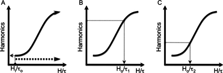
The temperature measurement method. The term “harmonics” on the ordinate refers either to the signal at a single harmonic frequency or to the ratio of the fifth and third harmonics. The harmonics are monotonic functions of the ratio , so each value of the harmonics yields a unique value of . By sweeping the drive amplitude at constant temperature , the calibration curve for the current size distribution is found as in (A). Subsequently, measurements of the harmonics at a selected drive field, , can be traced through the calibration curve to yield values of , e.g., and in (B) and (C), respectively, from which the current temperatures, and , can be found.
This method allows a good deal of flexibility to measure the temperature in a variety of settings and applications. If antibody targeted nanoparticles are employed, the size distribution of the bound nanoparticles might be different from that injected; e.g., if the larger nanoparticles are not able to diffuse as thoroughly as the smaller ones. The amplitude of the sinusoid in the Langevin function, , can be changed after the nanoparticles are bound in vivo by varying the amplitude of the applied field, , to map out the values of the harmonics that will be generated at other temperatures. This forms a calibration curve for any subsequent changes in temperature. Because the harmonics themselves and the ratios of the harmonics are monotonic with for any size distribution, once the calibration curve is known one subsequent measurement during heating or cooling will uniquely determine the temperature. Alternatively, if the calibration curve is known prior to administration, the temperature can be found for all subsequent measurements as long as the size distribution and binding do not change.
III. RESULTS
Simulations of the magnetization for 10 nm iron oxide nanoparticles using Eq. (2) are shown in Fig. 3, and the simulations for a log-normal distribution with mean of 40 nm and a standard deviation of 10 nm using Eq. (4) are shown in Fig. 4. The third and fifth harmonics and the ratio of the fifth and third harmonics are all monotonically increasing with . Further, it is shown that the monotonic relationship is preserved if nanoparticles of different sizes or size distributions are present. The monotonic relationship also holds for other common size distributions such as normally distributed nanoparticles.
FIG. 3.

Left: The calculated signal at the third and fifth harmonic frequencies as a function of the amplitude of the Langevin function . Decreasing temperature increases . For 10 nm iron oxide nanoparticles at room temperature with a 20 mT driving field, is roughly unity. The signal increases with decreasing temperature. Right: The ratio of the signals at the fifth and third harmonic frequencies as a function of the amplitude of the Langevin function, . The ratio increases monotonically with increasing amplitude but the sensitivity is uneven.
FIG. 4.

The same type of curve as shown in Fig. 3 but calculated for a wide log-normal size distribution: A mean of 20 nm and a standard deviation of 10 nm. Again, both the harmonics and the ratio increase monotonically with increasing Langevin function amplitude corresponding to the range of 0–10 mT/°K.
The data shown in Figs. 5–7 were taken with a 1470 Hz, 8.5 mT drive field. The harmonics resulting from amplitude variation and temperature variation are plotted in Fig. 5. There is a significant difference for higher temperatures, i.e., smaller values of for the individual harmonics. The general shape of the curves is similar to what would be expected based on the simulations in Figs. 3 and 4. We speculate that this is caused by the changes in the bulk magnetization in the coefficient outside the Langevin function in Eq. (2). The effect is not present for the ratio of the harmonics shown in Fig. 6. The bulk saturation magnetization outside the Langevin function cancels in the ratio and temperature variation mimics amplitude variation very closely. Figure 7 shows the accuracy of the temperature estimation compared to thermometer measurements. The standard deviation of the error and the rms error were both 0.3 °K (0.1%). The maximum error is 0.7 °K (0.2%). The reproducibility of the measurements of the harmonics was very high: 0.11% for the third harmonic and 0.13% for the fifth harmonic. The reproducibility of the ratio of the harmonics was better, 0.018%, probably because the variations in position of the sample show up in the harmonics but are canceled in the ratio. The error in the temperature measurement was less than 0.5 °K. The sample lost heat when it was removed from the water bath but at less than 0.15 °K per second. The data were taken after the sample was out of the water bath for a few seconds at most and we allowed for some cooling by removing the sample when it was a few tenths of a degree hotter than the desired temperature. Because the measurement errors were so small, we did not include error bars in the figures.
FIG. 5.

Measurements of the third harmonic (left axis) and the fifth harmonic (right axis) for different values of drive field amplitude and temperature. The calibration curve was taken by varying the amplitude of the drive field (solid and dashed lines). The temperature variation data (circles and plus symbols) followed the calibration curve quite well. The curves for both harmonics show that the temperature and drive field amplitude are not interchangeable at higher temperatures. The data were corrected for drive field amplitude using a coil outside the drive coil that measured the drive field.
FIG. 6.

The ratio of the measurements of the fifth and the third harmonics for different values of drive field amplitude and temperature. The curves show that for the ratio of the harmonics, the temperature and drive field amplitude are essentially interchangeable. The data were corrected for drive field amplitude using a coil outside the drive coil that measured the drive field.
FIG. 7.

The temperature measured using the method presented here compared to the thermometer reading. The nanoparticle temperature was accurate over the range of temperatures used. The sample size was small enough that the temperature was not stable for higher temperatures.
Although the stability of the apparatus is high, sensitivity must be maximized to measure the signal from molecular imaging concentrations of nanoparticles. The sensitivity can probably be improved significantly because most of the variation is drift over several minutes rather than random variation. We have done a first order correction for the drift of the power amplifier by using a pickup coil outside the drive coil to monitor the applied field and correct the measured signal for the drift. However, we believe that the electronics can be made more stable allowing still higher accuracy. For example, reducing the harmonic distortion of the amplifier is possible using a better amplifier and a drive coil with a higher Q. Monitoring the temperature of the pickup coil and improving the mutual inductance between the pickup coil and the balancing coil would also improve the stability and sensitivity. The functional form of the temperature correction of the bulk saturation magnetization also adds another element of uncertainty in the estimate. We found that a was 1.65 (Ref. 33) rather than the more common value of .31,32 We looked at four nanoparticle samples that had essentially the same value of a for lower frequencies, below 2 kHz, but diverged significantly for frequencies in the 10–15 kHz range. The blocking frequency suggests that the effect might be related to aggregation but we were not able to verify differences between the samples using electron microscopy. It is possible that a will resolve to in vivo when there is little aggregation or it may require a calibration at two temperatures for each sample prior to use to improve accuracy. The use of the more common value of increased the standard deviation in the error to 2.4 °K (0.8%).
IV. DISCUSSION
The methods of measuring temperature described could be productively employed in conjunction with any heating method but it should be especially well suited to methods involving nanoparticle heating. The first approach would be to alternate periods of heating with high applied fields with periods where the temperature is measured with lower amplitude fields. The applied fields during the next period of heating can then be modified to better approximate the desired temperature.
The capability to measure the temperature during heating would be very important because it would allow us to explore heating over time and distance scales that cannot be achieved otherwise. Temperature differences between the nanoparticles and the surrounding fluid could then be observed. However, it is unclear whether good temperature measurements can be made during heating with the same applied fields used to heat the nanoparticles. The applied fields employed to heat a single size of nanoparticles would place the harmonics in the relatively flat, asymptotic portion of the curves shown in Fig. 3. Figure 4 shows that the asymptotic region for a nonuniform size distribution is not as prominent, so it might still be possible to measure using the same fields that are used to heat the nanoparticles. In that case, the larger nanoparticles would be saturated but the smaller ones would still produce signal. Clearly, the temperature can be monitored in real time during heating if the heating is achieved via another mechanism such as focused ultrasound or laser light absorption.
A calibration curve can be generated at any time by sweeping through the amplitude of the applied harmonic field at a known temperature. Changes in temperature can then be estimated from the measured magnetization and the calibration curve. The calibration curve can be found for the specific size distribution of targeted nanoparticles deposited in vivo at a specific site or it can be updated at a later time if the size distribution might change due to washout or other effects.
The factors affecting the magnetization as a function of temperature should be explored more fully. The sensitivity of the constants a and b in Eq. (5) to aggregation, viscosity, and binding should be studied to understand the limitations of the method for various applications. For example, some cancer cells collect nanoparticles into vesicles relatively swiftly, which would increase aggregation and possibly impact the temperature estimate. Preliminary results indicate that the method works well for solutions with different viscosities as long as the frequency is above roughly 1 kHz for the size of nanoparticles we used. At lower frequencies, viscosity does affect the signal because Brownian motion becomes more significant than Neél relaxation. However, these are preliminary results and the effects of aggregation, viscosity, binding, and drive field amplitude and frequency should be explored further. The effects of factors like those are probably the largest source of error in the temperature estimation because the reproducibility is quite good.
Although we have not applied the methods described here in an imaging venue, the extension to producing temperature maps is reasonably straightforward. The most obvious way to extend the methods demonstrated to imaging temperature is to use the original MPI method of generating signal from a “field-free point” where the bias field is zero or very small.26 Then both harmonics can be imaged independently and the temperature calculated at each pixel in the image. Less than 1 mm spatial resolution has been achieved35 and MPI may be capable of microscopic applications but it is not known what spatial resolution can be achieved. However, it would also be useful to extend the temperature estimation to regimes where there is a static field because very large fields might be required to saturate most nanoparticle size distributions.28 Therefore, methods to estimate the temperature in the presence of a bias field would be important.
The impact of the method will ultimately depend on many factors including the success of antibody targeting methods and the success of MPI. However, the technology has clear potential in heating applications including magnetic nanoparticle hyperthermia, other hyperthermia methods, and ablation methods. The estimation of nanoparticle temperature is equivalent to estimating Brownian motion so it should be possible to estimate nanoparticle binding energy and the bound fraction using these methods. Estimating the binding is perhaps more important than estimating temperature because there are no good methods of measuring binding kinetics including binding energies and rate in vivo. Applications where the antibody binding kinetics needs to be separated from the nanoparticle perfusion should be enabled using this method. The distribution of nanoparticles present after a certain period is really a function of two factors: The blood supply to the tissue and the number of receptors present. Measuring the fraction of nanoparticles that are bound at any given time provides extra information that could prove to be extremely valuable.
V. CONCLUSIONS
The magnetization produced by nanoparticles is a balance between the magnetic forces aligning the nanoparticle magnetizations and thermal motion working to randomize the magnetizations. The ratio of the fifth and the third harmonics monotonically increases with the ratio of applied field and a variable that is a monotonic function of temperature and includes the temperature effects on the bulk saturation magnetization. Therefore, by varying the amplitude of the drive field at a known temperature, a calibration curve is formed for that sample of nanoparticles. Subsequently, each measurement of the ratio of the harmonics can be traced back through the calibration curve and the drive field to the temperature. The method is flexible and effective at measuring the temperature remotely and with relatively high accuracy; the standard deviation was 0.3 °K using the current apparatus. The temperature effects on the bulk saturation magnetization can be largely calibrated out because the functional form is known and the requisite constants are known from the literature or, for improved accuracy, they can be estimated for each sample.
REFERENCES
- 1.Pankhurst Q. A., Connolly J., Jones S. K., and Dobson J., “Applications of magnetic nanoparticles in biomedicine,” J. Phys. D 10.1088/0022-3727/36/13/20136, R167–R181 (2003). [DOI] [Google Scholar]
- 2.Cline H. E., Schenck J. F., Watkins R. D., Hynynen K., and Jolesz F. A., “Magnetic resonance-guided thermal surgery,” Magn. Reson. Med. 10.1002/mrm.191030011530, 98–106 (1993). [DOI] [PubMed] [Google Scholar]
- 3.Jolesz F. A. and Blumenfeld S. M., “Interventional use of magnetic resonance imaging,” Magn. Reson. Q. 10, 85–96 (1994). [PubMed] [Google Scholar]
- 4.Palussiere J., Salomir R., Le Bail B., Fawaz R., Quesson B., Grenier N., and Moonen C. T. W., “Feasibility of MR-guided focused ultrasound with real-time temperature mapping and continuous sonication for ablation of VX2 carcinoma in rabbit thigh,” Magn. Reson. Med. 10.1002/mrm.1032849, 89–98 (2003). [DOI] [PubMed] [Google Scholar]
- 5.Quesson B., de Zwart J. A., and Moonen C. T. W., “Magnetic resonance temperature imaging for guidance of thermotherapy,” J. Magn. Reson Imaging 12, 525–533 (2000). [DOI] [PubMed] [Google Scholar]
- 6.Mathews H. H. and Long B. H., “Minimally invasive techniques for the treatment of intervertebral disk herniation,” J. Am. Acad. Orthop. Surg. 10, 80–85 (2002). [DOI] [PubMed] [Google Scholar]
- 7.Rose S. C., Thistlethwaite P. A., Sewell P. E., and Vance R. B., “Lung cancer and radiofrequency ablation,” J. Vasc. Interv. Radiol. 17, 927–951 (2006). [DOI] [PubMed] [Google Scholar]
- 8.Steiner P., Botnar R., Goldberg S. N., Gazelle G. S., and Debatin J. F., “Monitoring of radio frequency tissue ablation in an interventional magnetic resonance environment. Preliminary ex vivo and in vivo results,” Invest. Radiol. 10.1097/00004424-199711000-0000432, 671–678 (1997). [DOI] [PubMed] [Google Scholar]
- 9.Steiner P.et al. , “Radio-frequency-induced thermoablation: Monitoring with T1-weighted and proton-frequency shift MR imaging in an interventional 0.5-T environment,” Radiology 206, 803–810 (1998). [DOI] [PubMed] [Google Scholar]
- 10.Jordan A., Scholz R., Wust P., Fahling H., and Felix R., “Magnetic fluid hyperthermia (MFH): Cancer treatment with AC magnetic field induced excitation of biocompatible superparamagnetic nanoparticles,” J. Magn. Magn. Mater. 10.1016/S0304-8853(99)00088-8201, 413–419 (1999). [DOI] [Google Scholar]
- 11.Le Bihan D., Delannoy J., and Levin R. L., “Temperature mapping with MR imaging of molecular diffusion: Application to hyperthermia,” Radiology 171, 853–857 (1989). [DOI] [PubMed] [Google Scholar]
- 12.Cetas T. C., “Will thermometric tomography become practical for hyperthermia treatment monitoring?” Cancer Res. 44, 4805–4808 (1984). [PubMed] [Google Scholar]
- 13.Kim S., “Liposomes as carriers of cancer chemotherapy: current status and future prospects,” Drugs 46, 618–638 (1993). 10.2165/00003495-199346040-00004 [DOI] [PubMed] [Google Scholar]
- 14.Weinstein J. N., Magin R. L., Yatvin M. B., and Zaharko D. S., “Liposomes and local hyperthermia: Selective delivery of methotrexate to heated tumors,” Science 10.1126/science.432641204, 188–191 (1979). [DOI] [PubMed] [Google Scholar]
- 15.Levy S., “Biophysical basis and cardiac lesions caused by different techniques of cardiac arrhythmia ablation,” Arch. Mal. Coeur Vaiss. 88, 1465–1469 (1995). [PubMed] [Google Scholar]
- 16.Madio D. P.et al. , “On the feasibility of MRI-guided focused ultrasound for local induction of gene expression,” J. Magn. Reson. Imaging 8, 101–104 (1998). 10.1002/jmri.1880080120 [DOI] [PubMed] [Google Scholar]
- 17.Ivkov R., DeNardo S. J., Daum W., Foreman A. R., Goldstein R. C., Nemkov V. S., and DeNardo G. L., “Application of high amplitude alternating magnetic fields for heat induction of nanoparticles localized in cancer,” Clin. Cancer Res. 11, 7093s–7103s (2005). 10.1158/1078-0432.CCR-1004-0016 [DOI] [PubMed] [Google Scholar]
- 18.DeNardo S. J., DeNardo G. L., Miers L. A., Natarajan A., Foreman A. R., Gruettner C., Adamson G. N. and Ivkov R., “Development of tumor targeting bioprobes (111In-Chimeric L6 monoclonal antibody nanoparticles) for alternating magnetic field cancer therapy,” Clin. Cancer Res. 11, 7087s–7092s (2005) 10.1158/1078-0432.CCR-1004-0022 [DOI] [PubMed] [Google Scholar]
- 19.Kong G., Braun R. D., and Dewhirst M. W., “Hyperthermia enables tumor-specific nanoparticle delivery: Effect of particle size,” Cancer Res. 60, 4440–4445 (2000). [PubMed] [Google Scholar]
- 20.Ito A., Kuga Y., Honda H., Kikkawa H., Horiuchi A., Watanabe Y., and Kobayashi T., “Magnetite nanoparticle-loaded anti-HER2 immunoliposomes for combination of antibody therapy with hyperthermia,” Cancer Lett. 212, 167–175 (2004). 10.1016/j.canlet.2004.03.038 [DOI] [PubMed] [Google Scholar]
- 21.O’Neal D., Hirsch L., Halas N., Payne J., and West J., “Photo-thermal tumor ablation in mice using near infrared-absorbing nanoparticles,” Cancer Lett. 209, 171–176 (2004). 10.1016/j.canlet.2004.02.004 [DOI] [PubMed] [Google Scholar]
- 22.Hirsch L. R., Stafford R. J., Bankson J. A., Sershen S. R., Rivera B., Price R. E., Hazle J. D., Halas N. J., and West J. L., “Nanoshell-mediated near-infrared thermal therapy of tumors under magnetic resonance guidance,” Proc. Natl. Acad. Sci. U.S.A. 10.1073/pnas.2232479100100, 13549–13554 (2003). [DOI] [PMC free article] [PubMed] [Google Scholar]
- 23.Keblinskia P., Cahill D. G., Bodapati A., Sullivan C. R., and Taton T. A. “Limits of localized heating by electromagnetically excited nanoparticles,” J. Appl. Phys. 10.1063/1.2335783100, 054305 (2006). [DOI] [Google Scholar]
- 24.Dahnke H. and Schaeffter T., “Limits of detection of SPIO at 3.0 T using T2* relaxometry,” Magn. Reson. Med. 10.1002/mrm.2043553, 1202–1206 (2005). [DOI] [PubMed] [Google Scholar]
- 25.Heyn C., Ronald J. A., Mackenzie L. T., MacDonald I. C., Chambers A. F., Rutt B. K., and Foster P. J., “In vivo magnetic resonance imaging of single cells in mouse brain with optical validation,” Magn. Reson. Med. 10.1002/mrm.2074755, 23–292006 [DOI] [PubMed] [Google Scholar]
- 26.Gleich B. and Weizenecker J., “Tomographic imaging using the nonlinear response of magnetic particles,” Nature (London) 10.1038/nature03808435(7046), 1214–1219 (2005). [DOI] [PubMed] [Google Scholar]
- 27.Weizenecker J., Borgert J., and Gleich B., “A simulation study on the resolution and sensitivity of magnetic particle imaging,” Phys. Med. Biol. 10.1088/0031-9155/52/21/00152, 6363–6374 (2007). [DOI] [PubMed] [Google Scholar]
- 28.Weaver J. B., Rauwerdink A. M., Sullivan C. R., and Baker I., “The spectral distribution of MPI signals in the presence of a static magnetic field,” Med. Phys. 10.1118/1.290344935, 1988–1994 (2008). [DOI] [PMC free article] [PubMed] [Google Scholar]
- 29.Kaiser R. and Miskoloczy G., “Magnetic properties of stable dispersions of subdomain magnetite particles,” J. Appl. Phys. 10.1063/1.165881241, 1064–1072 (1970). [DOI] [Google Scholar]
- 30.Herzer G., “Grain size dependence of coercivity and permeability in nanocrystalline ferromagnets,” IEEE Trans. Magn. 10.1109/20.10438926, 1397–1402 (1990). [DOI] [Google Scholar]
- 31.Martınez B., Roig A., Obradors X., Molins E., Rouanet A., and Monty C., “Magnetic properties of γ-Fe2O3 nanoparticles obtained by vaporization condensation in a solar furnace,” J. Appl. Phys. 10.1063/1.36112579, 2580–2586 (1996). [DOI] [Google Scholar]
- 32.Shendruk T. N.et al. , “The effect of surface spin disorder on the magnetism of γ-Fe2O3 nanoparticle dispersions,” Nanotechnology 10.1088/0957-4484/18/45/45570418, 455704–455710 (2007). [DOI] [Google Scholar]
- 33.Caizer C., “Deviations from Bloch law in the case of surfacted nanoparticles,” Appl. Phys. A: Mater. Sci. Process. 10.1007/s00339-003-2471-380, 1745–1751 (2005). [DOI] [Google Scholar]
- 34.Weaver J. B., Rauwerdink A. M., Trembly B. S., and Sullivan C. R., “Imaging magnetic nanoparticles using the signal’s frequency spectrum,” Proc. SPIE 6916, 6916–6935 (2008). [Google Scholar]
- 35.Gleich B., Weizenecker J., and Borgert J., “Experimental results on fast 2D-encoded magnetic particle imaging,” Phys. Med. Biol. 53, N81–N84 (2008). 10.1088/0031-9155/53/6/N01 [DOI] [PubMed] [Google Scholar]