In situ microfluidic dialysis for biological small-angle X-ray scattering

A remote-controlled microfluidic device for protein solution concentration and buffer exchange, simultaneous with small-angle X-ray scattering and ultraviolet absorption measurements, is presented.

Abstract

Owing to the demand for low sample consumption and automated sample changing capabilities at synchrotron small-angle X-ray (solution) scattering (SAXS) beamlines, X-ray microfluidics is receiving continuously increasing attention. Here, a remote-controlled microfluidic device is presented for simultaneous SAXS and ultraviolet absorption measurements during protein dialysis, integrated directly on a SAXS beamline. Microfluidic dialysis can be used for monitoring structural changes in response to buffer exchange or, as demonstrated, protein concentration. By collecting X-ray data during the concentration procedure, the risk of inducing protein aggregation due to excessive concentration and storage is eliminated, resulting in reduced sample consumption and improved data quality. The proof of concept demonstrates the effect of halted or continuous flow in the microfluidic device. No sample aggregation was induced by the concentration process at the levels achieved in these experiments. Simulations of fluid dynamics and transport properties within the device strongly suggest that aggregates, and possibly even higher-order oligomers, are preferentially retained by the device, resulting in incidental sample purification. Hence, this versatile microfluidic device enables investigation of experimentally induced structural changes under dynamically controllable sample conditions.

1. Introduction  

Small-angle X-ray scattering (SAXS), an increasingly popular technique for obtaining low-resolution structural information on biomacromolecules in solution, profoundly complements other techniques for structural analysis of biomacromolecules, such as crystallography and nuclear magnetic resonance. The versatile sample handling often makes SAXS the tool of choice for analyzing the structural changes of proteins in response to variations in their experimental environment.

The constant demand for lower sample consumption and more advanced ‘on-the-fly’ sample processing immediately before or during an X-ray exposure makes microfluidics a valuable future tool at SAXS beamlines. Microfluidic devices, with their modular nature, offer advanced liquid sample handling and the potential for a high level of integration of common laboratory functions. These chips are also known as lab-on-a-chip devices. Several successful microfluidic setups on SAXS stations have been presented in the literature, mostly focusing on mixing and/or high-throughput sample delivery (Pollack et al., 1999 ▶; Akiyama et al., 2002 ▶; Uzawa et al., 2004 ▶; Otten et al., 2005 ▶; Marmiroli et al., 2010 ▶; Toft et al., 2008 ▶).

The potentially wide variety of experimental conditions that may promote structural changes in a given protein solution are often unknown prior to the experiment. Thus, it is a requisite to analyze the structural state of a given protein under a large number of experimental conditions (Toft et al., 2008 ▶; Lafleur et al., 2011 ▶). Conventional biological SAXS experiments also require exposure at multiple protein concentrations. It is good practice to collect data at a minimum of three different concentrations to ensure the absence of interparticle interference and concentration-dependent oligomerization in the scattering data [for general guidelines, see e.g. Jacques et al. (2012 ▶)]. Protein samples are hence typically concentrated prior to data collection and data from a dilution series are recommended.

An automated lab-on-a-chip microfluidic sample preparation system for SAXS has recently been presented (Toft et al., 2008 ▶; Nielsen, 2009 ▶; Lafleur et al., 2011 ▶). This chip enabled automated mixing of samples and featured a sample X-ray chamber with fiber optics for integrated ultraviolet (UV) measurements. The structural space of a therapeutically relevant cytosolic signaling protein was successfully explored using the mixing chip (Møller et al., 2013 ▶). In both experiments, it was evident that several factors, including protein concentration, influence the oligomeric state of the biomacro­molecules, in either a reversible or an irreversible fashion. Additionally, the requirement of high starting concentration of the protein solution can promote protein aggregation and may trap the protein in irreversible and often biologically nonrelevant conformations. Thus, it is desirable to conduct SAXS experiments from initially low concentrations and to increase the concentration gradually while monitoring potential structural changes.

Several groups have presented microfluidic devices for the concentration of solutions. Khandurina et al. (2000 ▶) demonstrated the use of a porous silicate membrane, allowing the diffusion of water molecules between liquid phases with high and low water activity, respectively. However, inconsistencies with the on-chip concentration performance were also reported. Wang et al. (2005 ▶) used a nanofluidic filter combined with electrokinetic trapping to achieve a millionfold concentration in protein solutions. Fabrication of this device involved forming micro- and nanochannels in the same device. Kim & Han (2008 ▶) have presented a microfluidic device in polydimethylsiloxane (PDMS) with self-sealed nanoporous junctions inside PDMS for concentration of protein solutions applying an electric field over the nanoporous junction. Charged molecules are translated along the electric field, thereby enabling a concentration of proteins at pH values differing from the theoretical pI. Kondapalli et al. (2011 ▶) presented a microfluidic device that by similar principles enables concentration of protein solutions via electric field flow over a polyacrylamide membrane that at the same time functions as an immune biosensor. These methods all include either advanced fabrication for the membrane part or the application of electric field flow. Kim et al. (2007 ▶) have a more straightforward approach to fabrication of a microfluidic device for protein solution concentration. By the use of a conventional dialysis membrane sandwiched between two PDMS sheets with microchannels, concentration of protein solutions using simple membrane diffusion was demonstrated.

Here, we present a microfluidic device that enables concentration screening of a given protein solution, following the basic principles described earlier in the literature (Kim et al., 2007 ▶). Importantly, the concentration device presented here is integrated with a SAXS data collection sample cell and the ability to monitor the UV signal of the concentrated sample. Thereby, the device allows monitoring of potential concentration-induced structural changes and/or aggregation. This combined microfluidic device facilitates concentration series or buffer exchange series on any SAXS beamline. The combination of the microfluidic device with automation of the coordinated fluidic control and beamline control and partially automated data-processing software enables the user to make ‘on-the-fly’ adjustments to the experimental conditions directly based on the observed data. This provides SAXS beamline users with an unprecedented flexibility for optimized data collection from a protein while concentrating the solution. As data can be automatically collected during the time it takes for the concentration to reach a steady state, this microfluidic device facilitates measurements with extremely fine incremental steps of concentration that would otherwise be very impractical to obtain by hand.

Field-flow fractionation (FFF) is an ultrafiltration-based separation technique that shares important features with the method discussed here (Fraunhofer & Winter, 2004 ▶). The application of pressure to one side of a membrane can reverse the normal diffusive flow and result in ultrafiltration (reverse osmosis in the case of salts). The asymmetrical flow variant (AF4) of the method utilizes a single membrane on one side of a wide (>1 cm) sample-flow channel, but the technique is typically optimized for separation rather than concentration (Williams, 2012 ▶). Nonetheless, the fact that flow near a membrane surface can separate species with varying diffusion rates has important implications for the method we discuss.

2. Materials and methods  

2.1. Fabrication  

The microfluidic dialysis design includes two separate modules: a dialysis chip where the actual dialysis occurs, and an exposure chip where UV absorption at 280 nm is monitored and a SAXS exposure cell is located. The modular design principle is implemented to allow modifications in one module (e.g. inclusion of longer or wider dialysis channels) without modification of the other module. The design of both chips is illustrated in Fig. 1 ▶. Both chips were cast in PDMS from molds created by micromilling into a polydimethyl methacrylate (PMMA) substrate. The dialysis chip can be produced at very low cost and is intended as a disposable device, meaning that a new chip is recommended if the user changes between different proteins to avoid contamination.

Figure 1.

Illustration of dialysis and exposure chip design. The setup consists of two microfluidic modules, the dialysis chip and the exposure chip. (a) The dialysis chip has two identical sides (albeit with varying channel depth) with channels for the polyethylene glycol and protein sample solution, respectively. The two sheets are clamped together with a dialysis membrane in between. (b) The outlet of the dialysis chip sample solution channel is connected to the sample inlet on the exposure chip. The exposure chip contains a UV cell and a SAXS exposure channel with a polystyrene (PS) window. An air inlet makes it possible to blow out old sample in the exposure channel and the UV cell.

The dialysis chip consists of two sheets of PDMS (Fig. 1 ▶ a), one with 223 mm-long, 1 mm-wide and 0.12 mm-deep channels [the channel for the polyethylene glycol (PEG) solution], and a second with identical channel design but with a depth of 0.05 mm (the channel for the protein solution). These dimensions were chosen on the basis of earlier studies of microfluidic dialysis chips (Kim et al., 2007 ▶) and the limitations of the available micromilling fabrication method. A regenerated cellulose dialysis membrane (SpectraPor 3, 3.5 kDa cutoff, Spectrum Laboratories Inc., Rancho Dominguez, CA, USA) is sandwiched in-between the two PDMS sheets and clamped together using two pieces of 5 mm-thick PMMA plate.

The exposure chip has a thickness of 1 mm, which provides an X-ray pathlength for the exposure channel (see Fig. 1 ▶ b) at an X-ray energy of 10 keV. Polystyrene (PS) of 25 µm thickness was used as window material for the SAXS exposure cell (ST311025 biaxially oriented, Goodfellow Corporation, Coraopolos, PA, USA). PS is easy to work with and has been shown to produce low scattering levels at small angles (Toft et al., 2008 ▶; Gillilan et al., 2013 ▶). The windows were clamped to each side of the exposure chip over the exposure channel using PMMA plates. The soft PDMS provides a good seal around the windows and prevents leaks. This exposure cell design facilitated manual removal of concentrated solution in the cell by simply removing the sample from the exposure cell outlet using a pipette. This is useful either for cleaning out the previous sample or for external confirmation of the concentration using a UV spectrometer (NanoVue, GE Healthcare Biosciences, Pittsburgh, PA, USA).

2.2. Fluidic control setup  

The dialysis chip and the exposure chip were connected with short tubing (∼10 cm) with an inner diameter of 0.1 mm. The PEG and protein solutions were introduced into the dialysis chip using glass syringes (Hamilton) mounted in remote-controlled syringe pumps (NE-500, New Era Pump Systems Inc., Farmingdale, NY, USA). The pumps were controlled with software (Python script) developed in-house (Toft et al., 2008 ▶).

2.3. Sample preparation  

To test the system, solutions containing lysozyme (buffer: 40 mM NaOAc, 50 mM NaCl, pH 4.0) or glucose isomerase (buffer: 10 mM HEPES, 1 mM MgCl₂, pH 7.0) were continuously pumped into the protein channel on the dialysis chip at a flow rate of 0.9–1 µl min⁻¹. A 100 mg ml⁻¹ PEG 20 000 solution, dissolved in the same buffer as the protein solution or water, was pumped in the opposite direction on the PEG side of the dialysis chip at a flow rate of 10 µl min⁻¹. At these flow rates the deformation of the dialysis channel, due to increased pressure, is negligible (Gervais et al., 2006 ▶). Before the dialysis membrane was clamped between the two PDMS sheets, it was soaked and rinsed in distilled water for a minimum of 30 min to rinse out the preservative (glycerin). The membrane was not allowed to dry, since this can affect the pore size.

2.4. UV measurements  

Concentration using the dialysis chip is not linear over time, and UV absorption at 280 nm monitored immediately prior to the SAXS exposure cell is thus useful, and in some cases essential, to determine the concentration of the protein solution before SAXS exposure. The concentration of the sample is important for determining the average molecular mass of the scatterer and hence to determine the average oligomeric state and/or confirming monodispersity during SAXS data analysis. The UV absorption was monitored using the UV cell on the exposure chip (see Fig. 1 ▶ b) following the same basic principles as given by Lafleur et al. (2011 ▶). Optical fibers with a 250 µm diameter were inserted into the 250 × 250 µm side channels on the exposure chip, giving a path length of 1 mm. The optical fibers were connected to a spectrometer and a deep UV source (AvaSpec 2048 and AvaLight-DH-S-DUV, Avantes Inc Broomfield, CO, USA). Software (Python script) developed in-house facilitated automated recording of the absorption at 280 nm as a function of time.

2.5. SAXS experiments  

The experiments were carried out on the SAXS stations F2 and G1 at the Cornell High Energy Synchrotron Source (CHESS). The beam size on both stations was 250 × 250 µm (FWHM) at the exposure cell with a flux of 9 × 10⁹ photons s⁻¹ and an energy of 9.881 keV on F2 and a flux of 3 × 10¹¹ photons s⁻¹ at an energy of 9.869 keV on G1. Exposure times were limited to 1–2 min on F2 and to 5 s on the G1 beamline to avoid radiation damage of the samples. Basic SAXS data processing including radial averaging, background subtraction and radius of gyration (R _g) estimates was performed using the open-source data reduction software RAW (Nielsen et al., 2009 ▶).

3. Results  

3.1. Reproducibility  

UV measurements were used to determine the reproducibility of the concentrations obtained using the dialysis chip in a continuous flow mode. Three successive experiments were performed by first filling the dialysis chip with protein sample and applying a sample flow rate of 1 µl min⁻¹ with the PEG flow rate at 10 µl min⁻¹. Each experiment continued for 45 min. Fig. 2 ▶(a) shows a slow concentration increase during the first 10 min, followed by a steeper increase from 20 to 45 min. The reproducibility of protein concentration was estimated using UV illumination, revealing a maximum standard deviation of 0.11 mg ml⁻¹. Estimated using these data, the total volume needed to perform a concentration series is 67 µl. This estimate includes the volume of the dialysis chip channel (11.15 µl), the dead volume from the end of the dialysis chip to the X-ray exposure cell (6 µl), the volume of the X-ray cell (1 µl) and the volume used during a concentration series (45 µl).

Figure 2.

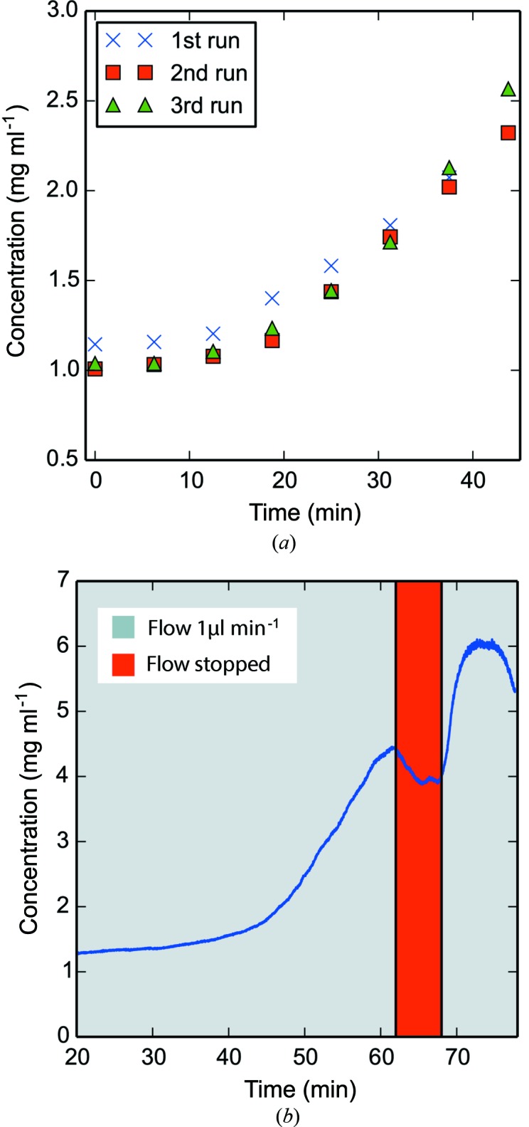
UV monitoring of protein concentration. (a) Plot of repeated UV-monitored continuous flow concentration series (n = 3). A lysozyme solution of 1 mg ml⁻¹ was pumped into the sample channel of the dialysis chip at a flow rate of 1 µl min⁻¹. PEG was pumped with the opposite flow direction into the PEG channel at 10 µl min⁻¹. The dialysis chip was flushed with sample after 45 min at high flow rate and the experiment was repeated. (b) Running the sample solution at a flow rate of 0.9 µl min⁻¹ will result in a fixed concentration after equilibration (in this case just before the red marking of ‘Flow stopped’ above). Halting the protein solution flow for a period of time can temporarily result in a higher protein concentration. In this case the pump was stopped for 7 min.

3.2. Concentration series  

Fig. 2 ▶(b) shows a concentration series recorded with UV absorption at 280 nm, using different flow rates than in Fig. 2 ▶(a). After a typical slow concentration phase, followed by the steeper increase in concentration, the curve begins to level out, i.e. resulting in a steady protein concentration. At this point, the pump injecting sample solution was paused for 7 min. A slight drop in concentration is seen after halting the pump, followed by a sharp increase in protein concentration immediately after restarting it. In the present experiment, the halted flow resulted in a further 150% concentration of the protein sample.

A SAXS concentration series on lysozyme is shown in Fig. 3 ▶, using a starting concentration of 2.2 mg ml⁻¹. The data reveal the concentration effect by continuous and halted flow. In both Figs. 3(a) and 3(b) (before and after background subtraction, respectively) we see a gradual rise in overall scattering intensity from light-green to dark-green curves, obtained with 5 min intervals. An approximate factor of three in concentration was obtained, while a factor of six was obtained after halting the flow for 10 min. The first measurement after restarting the pump is plotted in light blue, and a gradual decrease in intensity is observed for the subsequent measurements (light-blue to dark-blue curves). SAXS data were not collected during the stopped flow, and a drop in concentration, as seen in the red box of Fig 2 ▶(b), is therefore not visible in the data.

Figure 3.

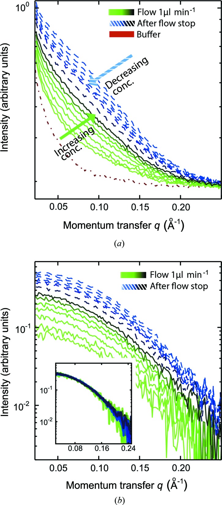
SAXS-monitored lysozyme concentration series. (a) The scattering curves obtained during data collection from a concentration series on lysozyme with an initial concentration of 2.2 mg ml⁻¹. Two different approaches were used. The green scattering curves (light green to dark green) indicate protein concentration obtained using continuous flow with a sample flow rate of 1 µl min⁻¹ and a PEG flow rate of 10 µl min⁻¹. SAXS data were collected at 5 min intervals. The sample flow was halted for 10 min. The blue scattering curves show the resulting abrupt concentration, when the sample flow was reinitiated at 1 µl min⁻¹, with subsequent dilution (light blue to dark blue). SAXS data (blue curves) were collected with 3 min intervals. The red curve is the scattering curve from buffer solution. SAXS data were not collected during the stopped flow. (b) The background-subtracted data. The inset shows the superimposed data curves after scaling for concentration.

3.3. Buffer exchange series  

Figs. 4 ▶ and 5 ▶ show data from concentration series where the PEG has been dissolved in water rather than buffer solution. Fig. 4 ▶ shows the gradually changing scattering curves from lysozyme at an initial concentration of 1 mg ml⁻¹, during concentration over a period of 80 min. A clear overall increase is seen in intensity over time (from protein concentration), but accompanied by the emergence of a downward turn in the scattering profile at lower q values. This downward trend is a well characterized signature of long-range interparticle repulsion in lysozyme solutions, which increases with decreasing ionic strength (Niebuhr & Koch, 2005 ▶; Shukla et al., 2008 ▶; Stradner et al., 2004 ▶). A buffer exchange has hence accompanied the protein concentration procedure. The change in buffer composition is also apparent at the widest scattering angles recorded, resulting in a mismatch of the background subtraction (shown in Fig. 5 ▶). This initial experiment hence clearly exposes the need to obtain scattering measurements also from the modified buffers when collecting SAXS data during buffer exchange.

Figure 4.

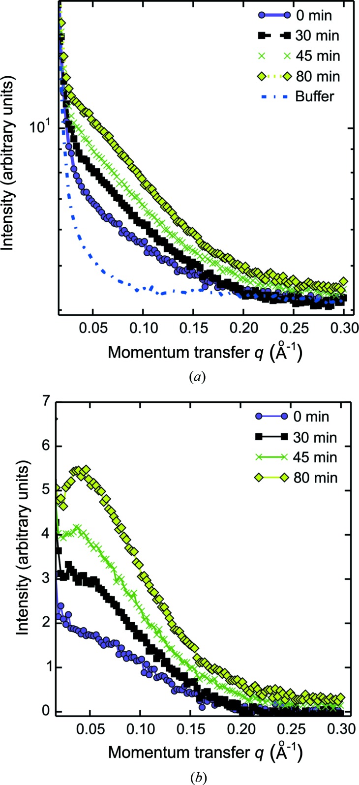
SAXS-monitored buffer exchange and concentration series. (a) SAXS curves from initially 1 mg ml⁻¹ lysozyme during concentration and buffer exchange. The blue scattering curve shows the data for the buffer solution. (b) Background-subtracted scattering intensity curves. There is a clear rise in intensity (due to protein concentration) and also a change in the scattering pattern at low q with increasing time, revealing an increase in the structure factors and the compromised background subtraction, owing to the changes in buffer composition over time.

Figure 5.

SAXS-monitored glucose isomerase (GI) concentration series. (a) Concentration of a glucose isomerase solution from 3.4 mg ml⁻¹ at t = 0 min (shown in purple) to 6.5 mg ml⁻¹ at t = 43 min (shown in black). The two corresponding buffer intensity curves are also plotted, one at t = 0 min (purple) and one at t = 43 min (black). The required volume was 40 µl from the first to the last measurement. The sample and the PEG solutions were injected at a rate of 1 µl min⁻¹ and SAXS data were collected every 5 min. The inset shows the gradual concentration of the protein sample. Buffer changes were induced during concentration in the dialysis chip using PEG in water, rather than PEG in the protein buffer. (b) Plot of background-subtracted intensity curves at 3.4 mg ml⁻¹ (purple) and 6.5 mg ml⁻¹ (black) using data from buffers exposed to the same dialysis period as the protein samples for the background-subtraction procedure. (c) For the starting solution at 3.4 mg ml⁻¹, R _g = 32.0 Å was determined [qR _g(min) = 0.45, qR _g(max) = 1.30]. (d) For the final solution at 6.5 mg ml⁻¹ R _g = 32.5 Å was determined [qR _g(min) = 0.70, qR _g(max) = 1.30].

3.4. Data quality after protein concentration and buffer exchange  

Fig. 5 ▶ illustrates an experiment similar to the lysozyme concentration and desalting using a glucose isomerase sample of an initial protein concentration of 3.4 mg ml⁻¹. Fig. 5 ▶(a) shows the first and last measurement of a concentration series and the inset shows the gradual increase in the scattering signal with time. It is noted that the scattering at medium and high q values from the buffer measurement for time t = 0 min is higher than the protein signal from glucose isomerase at t = 43 min, thereby again illustrating the need for the measurement of the correct buffer background, and also revealing the efficiency of buffer exchange across the membrane. An adequate buffer measurement after buffer exchange is obtained by running buffer through the sample channel at the same flow rate as for the protein sample, which hence produces a buffer measurement that matches the concentrated sample at t = 43 min. The background-subtracted data are shown in Fig. 5 ▶(b). It is noted that the two background-subtracted scattering curves are indistinguishable when scaled for concentration (in this case a factor of 1.7). This proves that the buffer-exchanged background measurement has been correctly performed.

After obtaining adequate buffer measurements (hence applying buffer exchange via dialysis), R _g was estimated for the scattering curve of the starting concentration (t = 0 min) and the scattering curve of the final concentration (t = 43 min) (see Figs. 5 ▶ c and 5d). For the starting concentration (3.4 mg ml⁻¹), R _g was estimated as 32.0 Å and for the final concentration (6.5 mg ml⁻¹) R _g was estimated as 32.5 Å. Both estimates are consistent with what is reported in the literature [R _g = 32.5 (7) Å; Mylonas & Svergun, 2007 ▶]. It is evident that the concentration and buffer exchange has not resulted in any unwanted protein aggregation and, most importantly, that the buffer match obtained by dialysis results in scattering data of adequate quality.

4. Fluid dynamics and transport  

4.1. Theory  

The small size scale and relatively slow flow rates encountered in many microfluidic applications render simulations of fluid flow well within the Stokes (creeping) flow regime. The Reynolds number for a flat channel, 1000 µm wide by 50 µm deep, carrying water at 1 µl min⁻¹ using kinematic viscosity υ = 1.5 × 10⁻⁶ m² s⁻¹ at 278 K and assuming a hydrolic diameter of 2 × 50 µm, is 0.02 << 1. Owing to the extreme scale difference (20:1) between width and depth of channels, we will confine our analysis here to only two dimensions: channel depth (y) and channel length (x). Under such conditions, the fluid velocity field u = (u _x, u _y) for a simple two-dimensional channel with one porous wall can be solved analytically (Appendix A ).

Longitudinal flow thus scales linearly to zero as all the buffer has leaked away by the time the balance point in the channel is reached. This is true in both directions. The transverse flow, u _y, is completely independent of x. The flow field is shown in Fig. 6 ▶(a) on an exaggerated scale for illustration, with the membrane being represented by a dashed line at y = 0. Because of conservation of volume in this incompressible system, the only flow that appears is transmembrane flow u _m. To simulate a finite-length channel with specified volumetric inlet flow

one simply selects the starting point x to give the desired value [x = 28 in Fig. 6 ▶(a)]. For a channel of length L having an entrance at x = x _en, the exit will be located at x = x _en − L > 0 [x = 5 in Fig. 6 ▶(a)]. Ideally, the concentration factor achieved as the sample passes from one end to the other would be f(x _en)/f(x _en − L) = x _en/(x _en − L), but Poiseuille flow causes fluid in the middle of the channel to move more rapidly than fluid near the membrane surface. Consequently, we can expect the concentration factor to have some dependency on the diffusion constant and on the channel dimensions. Understanding chip performance thus requires a more detailed examination of convection and diffusion.

Figure 6.

Fluid simulations inside a dialysis chip. (a) Simulated fluid velocity field inside the chip. Scales and flows are exaggerated for the purpose of illustration. Vertical lines mark inlet and outlet locations. Fluid velocity is strictly vertical at the balance point (x = 0), a virtual location normally outside the chip. The dashed line (y = 0) identifies the membrane surface. (b) Simulations of steady-state concentration profiles for a rapidly diffusing lysozyme-like protein (D = 10⁻⁶ cm² s⁻¹). (c) Simulations of steady-state concentration profiles for a slowly diffusing aggregate (D = 10⁻⁸ cm² s⁻¹). Species slower than D = 5 × 10⁻⁸ cm² s⁻¹ show a visible concentration gradient within the 50 µm channel.

Protein concentration changes within the microfluidic channel are governed by the convection–diffusion equation:

We assume that concentration c(x, y, t) does not affect the density or the Newtonian flow properties of water. Equation (2) also assumes that diffusion, D, is constant. A very important characteristic of sample behavior near a membrane can easily be seen by solving the one-dimensional steady-state version of equation (2) for a finite amount of sample experiencing constant transmembrane buffer flow u = (0, u _m):

Simple integration of equation (3) along with the condition of finite total concentration yields

which can be solved directly for concentration:

Equation (4) is equivalent to the so-called Robin boundary condition, but reduces to the more familiar Neumann condition when u _m = 0 (Deen, 1998 ▶). In the absence of flow (impermeable, no-leak walls), concentration gradients must therefore vanish at the walls. However, at permeable walls, the convective flux combines with diffusion to result in an exponential decay of concentration (recall that u _m < 0), the width of which depends upon the diffusion constant of the species involved. This is a well known and important phenomenon in field-flow fractionation (Giddings, 1993 ▶); massive, slowly diffusing species concentrate closer to the membrane than lighter, more rapidly diffusing species. As we shall see in a moment, this phenomenon has important implications for chip-based dialysis as well.

The dialysis channel is initially filled with dilute sample: c(x, y, t) = c ₀ for x _en − L ≤ x ≤ x _en and 0 ≤ y ≤ d. During simulation, an inlet boundary condition is imposed to simulate the constant flow of fresh sample into the channel: c(x _en, y) = c ₀ for 0 ≤ y ≤ d. The upper wall y = d is impermeable with u _x = u _y = 0. The lower wall, y = 0, also has u _x = 0 and experiences a constant transmembrane buffer flow u _y = u _m but is otherwise impermeable to solute. The outlet boundary condition at x = x _en − L allows free diffusion and convection outwards.

To solve equation (2) numerically, we utilize the finite volume method (Versteeg & Malalasekera, 2007 ▶) as implemented in the package FiPy (release 3.0; Guyer et al., 2009 ▶). The steady-state form of equation (2) was solved using the exponential convection term option with equations (12) and (13) as input. An explicit source term was introduced to precisely cancel outward diffusion and convection at the outlet, simulating free flow as described in the FiPy documentation (http://www.ctcms.nist.gov/fipy/). The simulation was conducted on a grid of 400 cells (x) by 50 cells (y). Convergence for steady-state solutions was assessed by varying the number of cells in the simulation. To assure accuracy for a wide range of simulation parameters, cell numbers well in excess of the necessary minimum were chosen.

The full transient form of equation (2) was solved on the same grid with the same parameters, but accurate time propagation required the use of a van Leer convection term with variable time steps (van Leer, 1979 ▶). The necessity of using this particular strategy in time propagation was seen in D = 0 test cases where pure translation of sample boluses is expected. Time steps were started at 0.018 s and doubled every 100 steps to a maximum of 1.152 s per step. In the upstream end of the tube, high longitudinal flow rates adjacent to very slow transmembrane flow rates initially require very fine time stepping, but steady-state conditions are reached very rapidly in those locations; consequently time steps can be increased once the steady state is achieved locally. Steady-state flow conditions progress down the channel with time, reaching the outlet last. The final states achieved in transient calculations agreed with those in the steady-state calculations.

4.2. Limitations and approximations  

As already mentioned, our simulations treat the wide but very shallow (20:1) dialysis channels as a two-dimensional system. Dialysis membranes are known to swell and deform some in reality, and consequently the true channel depth is not a precisely known quantity. A more elaborate treatment would also model the PEG channel as well as the porous membrane (Tuhy et al., 2012 ▶). Further, the microfluidic channels are not straight but folded to fit on the chip. Such turns in the channel have a well known distorting influence in microfluidics known as the racetrack effect (Kirby, 2010 ▶). Halted-flow experiments may be further influenced by the so-called compliance of the device (elastic response to changes in pressure). Higher concentrations of protein may also introduce interesting non-Newtonian/rheological properties into the simulation. The formation of so-called polarization layers is a much-studied phenomenon in ultrafiltration that is closely related to this work (Song & Elimelech, 1995 ▶; Pignon et al., 2012 ▶). Transmembrane flow, which we have assumed constant in this work, can be impeded in the polarization layer by a variety of factors when protein solution becomes highly concentrated. The point of these simulations, however, is not to model the experimental system in complete detail, but rather to clarify the essential physics at work and to understand how various design parameters influence the performance of the chip.

4.3. Simulation results  

The parameters for this simulation were chosen to approximately model the experimental chip setup (Table 1 ▶). Although outlet flow was not measured directly in these experiments, the observation that it stopped altogether for inlet flows less than 0.9 µl min⁻¹ gives some approximate indication of the transmembrane flow rate. At 0.8 µl min⁻¹ transmembrane flow, the outlet flow in our simulation gave both a reasonable refresh time for exposed sample in the X-ray beam and a steady-state concentration factor close to that actually observed in Fig. 2 ▶(b) during the first 60 min of operation. To move sample from the end of the channel to the X-ray cell, a dead volume of ∼6 µl, required nearly 27 min (Table 1 ▶), and consequently the simulations of time to reach steady state are most meaningfully compared with the range from 30 to 60 min in Fig. 2 ▶(b). Stopped flow is not modeled in these simulations.

Table 1. Simulation parameters.

Flow at inlet (µl min−1)	1.02
Flow at outlet (µl min−1)	0.23
Transmembrane flow (u m) (µl min−1)	0.80 (0.0215 cm h−1)
Inlet to balance point (cm)	28.6
Channel dimensions (cm)	23.3 × 0.1 × 0.005
Idealized concentration factor	4.5
Time for X-ray cell refresh (min)	2.21 (0.5 µl)
Time from outlet to X-ray cell (min)	26.58 (6.0 µl)

Figs. 6 ▶(b) and 6 ▶(c) show examples of the steady-state concentration gradient within the channel for proteins of two very different diffusion constants. In Fig. 6 ▶(b), a rapidly diffusing protein such as lysozyme (D ≃ 10⁻⁶ cm² s⁻¹) fills the narrow 50 µm channel near the outlet. A much more slowly diffusing protein or aggregate (D ≃ 10⁻⁸ cm² s⁻¹) shows a distinct concentration gradient, which is highest near the membrane surface (Fig. 6 ▶ c). The color bar on the right-hand side of Fig. 6 ▶ gives an indication of concentration range.

The full transient form of equation (9) is solved in Fig. 7 ▶ for a range of diffusion constants from 10⁻⁶ cm² s⁻¹ down to 10⁻⁹ cm² s⁻¹. Above D = 5 × 10⁻⁸ cm² s⁻¹, all curves show the same behavior, in which the steady state with idealized concentration factor of 4.5 is reached in 20 min (Fig. 7 ▶ a). Below D = 5 × 10⁻⁸ cm² s⁻¹, samples take progressively longer to reach the steady state, but when they do, the final concentration factor is higher. Fig. 7 ▶(b) reveals that cross-sectional concentration gradients near the outlet go from flat to exponential as they cross the D = 5 × 10⁻⁸ cm² s⁻¹ threshold. Large proteins or aggregates thus show diffusion-limited behavior in the chip, leading to higher concentrations in slower parts of the flow field. As a result, the larger the protein, the more delayed the arrival. All sample components above a certain threshold diffusion rate will arrive at the outlet at the same time and be concentrated to the same extent (so long as the channel is much longer than the characteristic diffusion time).

Figure 7.

Theoretical chip performance with various types of proteins. Number labels are diffusion constants in cm² s⁻¹. (a) Time to reach steady state is 20 min (effect of dead volume not shown) for fast-diffusing proteins. Slow proteins and aggregates take more than 30 min but are more concentrated when they reach the outlet. (b) Steady-state concentration gradient at outlet. For proteins faster than a certain threshold (8.5 × 10⁻⁸ cm² s⁻¹), the profile is flat and the final concentration and equilibration time are independent of diffusion. Slow proteins or aggregates are diffusion-limited and concentrate in the slow-moving flow near the membrane surface. As such, they take much longer to elute but ultimately reach a higher concentration.

5. Discussion  

In order to adequately benefit from SAXS beamtime at the large scale facilities, and to optimize the spending of precious macromolecular samples, it is highly desirable to develop advanced sample handling devices. The microfluidic device presented here requires minimal sample handling and enables ‘on-the-fly’ protein concentration and buffer exchange. The design presented here combines a UV absorption cell and a SAXS measurement cell in an exposure chip module separate from a simple dialysis module. This proof of concept setup shows how structural changes and small changes in the experimental conditions are readily monitored using UV and SAXS.

Microfluidic devices for enrichment of protein solutions have previously been reported (Khandurina et al., 2000 ▶; Wang et al., 2005 ▶; Kim & Han, 2008 ▶; Kondapalli et al., 2011 ▶), but these devices demand either very complex fabrication techniques or the use of electric field flow. The presented microfluidic chips can be treated as disposables because of the low costs of PDMS and fast production, as reported earlier (Kim et al., 2007 ▶). Furthermore, the combination of an automated microfluidic device and associated partially automated software provides the user with structural feedback immediately during data collection, exposing potential structural changes caused by the experimental changes in the sample. The ease of adjustment of the experimental conditions in the microfluidic setup provides the user with the flexibility to respond to and optimize data collection during beamtime.

5.1. Flowrate/exposure times and radiation damage  

The dialysis chip enables SAXS experiments conducted from protein samples of initially low concentrations that are then gradually enriched via a gentle dialysis approach.

By starting with dilute protein and working upward in concentration while performing SAXS measurements, potential structural changes are monitored and the initial formation of possibly irreversible aggregation is readily detected. By this principle, it is ensured that a SAXS measurement is performed at the highest possible protein concentration devoid of unwanted effects such as aggregation and structure factor distortions. Aggregation can also be a time-dependent phenomenon. The ability to perform ‘on-the-fly’ measurement is an absolute advantage, rather than first concentrating (off-line) and then transporting the sample to the beamline for measurements. Such concentration series are also expected to be valuable in the analysis of concentration-dependent oligomerization or molecular crowding effects, where the maximally achievable concentration is unknown.

Owing to the minute amounts of sample that are consumed on the dialysis chip, fast sample movement is not possible during exposures. This makes the sample sensitive to radiation damage and sets a practical limit for the exposure time. The practical exposure limit is dependent on the intensity of the X-ray beam at the beamline. It is also possible to vary the actual X-ray dosage on the sample by modifying the focus and therefore the size of the X-ray beam at the sample position. In the present experiments, protein aggregation was not detected and hence radiation-induced aggregation has not been a problem. By using pixel array detectors, very low timeframes of sample exposure may be used, thereby enabling direct monitoring of potential X-ray-induced sample damage.

5.2. Concentration series  

Concentration of protein solution was achieved using both continuous flow and halted (stopped) flow. A factor of three–four in concentration was achieved with continuous flow. The maximum concentration was achieved using a combination of continuous flow and halted flow where a factor of six in concentration was reached. Initially, the concentration remains flat until ∼6 µl of dead volume is expelled. A maximum in concentration (the steady state) is seen when the slope of the curve starts to decrease. However, halting the flow at this point and waiting several minutes caused a temporary increase of the concentration. In effect, the balance point of the device resided inside the chip for that time. Once flow resumes, a bolus of higher concentration is expelled, creating a new temporary plateau. The small decrease in concentration right after the stopping of the pump is likely to be due to dilution by previously measured sample in the UV exposure cell.

In an attempt to obtain the maximum protein concentration, the protein solution flow rate was kept at the lowest possible, but still allowing the protein solution to propagate towards the exposure cell with enough sample volume in a reasonable timeframe, i.e. close to the rate of solute transport across the dialysis membrane. For the parameters used in these studies, the optimized flow rate was found to be around 1 µl min⁻¹. At flow rates below ∼0.9 µl min⁻¹ the sample flow rate is exceeded by the rate of buffer transportation through the membrane, resulting in no or reversed propagation of the sample in the protein channels.

5.3. Desalting of protein solution and background subtraction  

The dialysis chip also facilitates the study of structural changes due to gradual changing of buffer components such as removal or addition of ions from the sample solution. It is important to note that the change of buffer conditions in a sample will also require the exact same changes to the buffer used for background subtraction when using SAXS. Here, we have shown that this can be obtained by exposing the buffer samples to the same microfluidic handling as for the protein solution.

Fig. 4 ▶ shows an example of gradual concentration and desalting of lysozyme. The results indicate a clear change in the lower-q area of the scattering curve, as would be expected from desalting because of the increasing structure factor effects (Shukla et al., 2008 ▶). It should be emphasized, however, that these structure factor changes are not monitored in detail, owing to the noted compromise in background subtraction when using the initial buffer measurement for this procedure only.

In contrast, we demonstrate (Fig. 5 ▶) how running the buffer through the chip while using the same flow rate as for the sample provides a buffer measurement that matches the sample measurement at a specific time (t). The data also clearly illustrate how reproducible scattering profiles can be extracted from glucose isomerase even after both concentration and buffer changes. This indicates that the protein did not experience damage (forming aggregates) either from the induced concentration and buffer exchange or from X-ray exposure. Additionally, and perhaps more importantly, the results demonstrate the reproducibility of dialysis, since we obtain a perfect background match from the buffer measurement on the same dialysis chip. However, it must be noted that this procedure doubles the demand in beamtime.

5.4. Dialysis, ultrafiltration and pressure balance  

Differences in osmotic pressure between the sample and the PEG solution drive the flow of buffer across the semipermeable membrane. PEG 20 000 provides a significant pressure differential of 152 kPa at 100 mg ml⁻¹ (Williams & Shaykewi, 1969 ▶), but PEG is also a very viscous fluid that can build up a significant pressure simply flowing through a channel. Internal channel pressure works in opposition to osmotic pressure in this case, potentially lowering the effective concentrating ability. Sufficient opposing pressure could, in fact, reverse the buffer flow (ultrafiltration). The resulting pressure gradient along the length of the channel could also introduce non­linearities in performance. The Hagen–Poiseuille formula, which relates pressure drop through a channel with flow rate and viscosity, has recently been modified to account for rectangular cross-sectional channels (Biral, 2012 ▶). Let Q be flow rate, L be channel length, and w and h be width and height, respectively (SI units). If μ is the dynamic viscosity (Pa s), then

For PEG 20 000 at 10% w/w, μ = 0.01 Pa s, an order of magnitude larger than water (Holyst et al., 2009 ▶). Conveniently, the density of PEG 20 000 is quite close to unity. At Q = 10.0 µl min⁻¹, the predicted pressure differential for PEG flow in the 0.12 × 1.0 × 220 mm channel is thus 2.8 kPa, about 2% of the osmotic pressure. The effect is insignificant in this experiment and can be ignored, but could easily become a factor of importance with longer narrower channels or higher PEG flow rates.

The range of possible osmotic pressures of protein solution relative to buffer is estimated using the simple Morse equation (Foley, 2013 ▶). For lysozyme (14.3 kDa at 1–6 mg ml⁻¹) osmotic pressures are estimated to range from 0.2 to 1 kPa, consistent with published values measured under higher salt conditions (Moon et al., 2000 ▶). Glucose isomerase (173 kDa) in the same range of concentrations yields even lower pressures (0.014–0.084 kPa). From the standpoint of dialysis, PEG solutions far exceed the necessary osmotic pressure difference to cause concentration. However, when expressed in units of mm H₂O (10 Pa ≃ 1 mm H₂O), it becomes evident that protein concentration and buffer exchange could be accomplished without PEG through the use of external pressure alone. Indeed, ultrafiltration has already been combined with SAXS measurements to probe the polarization layers in colloidal dispersions and micelles (David et al., 2008 ▶; Pignon et al., 2012 ▶). The extent to which behavior in those regimes applies to typical protein solutions should be a fruitful area for future investigation.

5.5. Fluid dynamics, transport and retention of aggregates  

Whether flow through the membrane is induced by osmotic pressure or external pressure, it has important hydrodynamic effects on proteins in the channel. FFF experiments have already demonstrated that species with different mass are naturally separated under these conditions (Giddings, 1993 ▶). In the AF4 method, samples flow along a single very wide (>1 cm) but shallow (<500 µm) channel defined on one side by a semipermeable membrane that admits only buffer. The transverse flow of buffer through the membrane combines with parabolic (Hagen–Poiseuille) flow tangent to the membrane to separate species with differing rates of diffusion. Though the channels in our dialysis chip are much narrower than typical AF4 configurations, the depth and flow parameters are comparable. Analysis of convection and diffusion phenomena within the chip shows that mass separation can indeed occur, and that larger particles such as aggregates will be significantly retarded. The present design, however, does not provide mass resolution for species with diffusion constants above D = 5 × 10⁻⁸ cm² s⁻¹. Most common proteins in their native oligomeric state will not be resolvable from their dimeric or tetrameric forms in this case. The choice of channel depth (50 µm here) is the most important design parameter influencing mass resolution. Future designs may be able to offer a greater degree of incidental sample purification.

6. Conclusion  

A microfluidic setup for remote-controlled and ‘on-the-fly’ dialysis and buffer exchange in combination with SAXS is presented. This proof of concept demonstrates how microfluidic dialysis, coupled with a SAXS/UV exposure cell, can be used for concentration-scanning series and for dynamically monitoring structural changes in response to changing buffer conditions. Rather than having to handle minute volumes of concentrated samples, the microfluidic dialysis starts with large volumes of dilute solution; this facilitates handling and reduces potential loss. The concentration factors (×4 to ×6) achieved in these preliminary experiments are promising and adequate for checking sample concentration dependence. On-chip UV absorption measurement permits real-time determination of sample concentration during the experiment, a necessary requirement for mass estimation. In buffer exchange experiments, a well matched buffer can be achieved by running a duplicate experiment with buffer instead of sample.

Because the sample may become highly concentrated near the dialysis membrane, a valid concern is whether or not the concentration process can induce aggregation. None has been observed at the levels of concentration achieved in these experiments. Further, detailed transport calculations strongly suggest that any aggregates that might be produced will be detained on the microfluidic chip. Thus, microfluidic dialysis may accomplish some sample purification as an unexpected side benefit.

The design presented here is readily implemented on a SAXS beamline. Easily changeable, low-cost membranes and disposable sample chips are compatible with a high-throughput environment. The high level of automation of the fluid control, data acquisition and initial data analysis allows the user to concentrate on the experimental design and initial conclusions, and hence promises an optimized use of often very precious protein samples. All software is freely available upon request.

Appendix A.

Under the assumption of viscous flow, the Navier–Stokes equations reduce to

where p is pressure, μ is dynamic viscosity and u = (u _x, u _y) is the vector field describing flow (Kirby, 2010 ▶). Introducing a scalar function Ψ(x, y) and using the transformation

pressure and viscosity drop out of the equation and one obtains the fourth-order two-dimensional biharmonic equation (Kirby, 2010 ▶)

For an infinite channel of depth d having one semipermeable side with outward flow u _m, we can impose no-slip boundary conditions at the walls: u _x(x, 0) = u _x(x, d) = 0. Further, there is no leakage at the top wall, u _y(x, d) = 0, and specified leakage at the bottom wall, u _y(x, 0) = u _m. Note that for concentration to occur in the chip, u _m is less than 0. We can further expect sample solution traveling in the positive x direction to eventually come to a stop as the net flow down the tube becomes equal to the net flow out of the membrane. For symmetry, we can assume that buffer solution is travelling in the negative x direction to meet up with the sample at x = 0. We refer to this location as the balance point. Generally, the balance point is a virtual location somewhere outside the dialysis chip downstream from the outlet. So at the stationary line x = 0 we have u _x(0, y) = 0 for both fluids. This symmetry actually places much stronger requirements on the solution of the equation. We can say that −u _x(−x, y) = u _x(x, y) and u _y(x, y) = u _y(−x, y). So u _x is an odd function and u _y is an even function. To understand how to apply these boundary conditions, it is necessary to expand the solution in terms of elementary functions with coefficients. Fortunately, one can accomplish this with a simple polynomial expansion:

Using transformation (8), we can impose the boundary conditions above. Since u _x is odd in x, a _0,1 = a _0,2 = a _0,3 = 0. Similarly, since u _y is even in y, a _2,0 = a _2,1 = a _2,2 = a _2,3 = 0. No-slip conditions at both walls results in a _1,1 = a _3,1 = 0, a _1,2 = −3/2a _1,3 d and a _3,2 = −3/2a _3,3 d. Similarly, no-leak conditions yield a _1,0 = 1/2a _1,3 d ³. Specified-leak conditions are only satisfied if a _3,3 = 0 and a _1,3 = −2u _m/d ³. Substituting these coefficients into equation (10), we obtain

and

It is easy to verify that the stream function Ψ obeys equation (9). The longitudinal fluid velocity u _x [equation (12)] is recognizable as the famous Poiseuille flow pattern, but modulated by a factor of x. Curiously, the two-dimensional flow field for a more symmetric channel having two porous walls has been solved, though apparently not in a simple closed analytic form such as we have presented here, but one requiring perturbation methods (Berman, 1953 ▶).

References

- Akiyama, S., Takahashi, S., Kimura, T., Ishimori, K., Morishima, I., Nishikawa, Y. & Fujisawa, T. (2002). Proc. Natl Acad. Sci. USA, 99, 1329–1334. [DOI] [PMC free article] [PubMed]
- Berman, A. S. (1953). J. Appl. Phys. 24, 1232.
- Biral, A. (2012). PhD thesis, Università degli Studi di Padova, Italy.
- David, C., Pignon, F., Narayanan, T., Sztucki, M., Gésan-Guiziou, G. & Magnin, A. (2008). Langmuir, 24, 4523–4529. [DOI] [PubMed]
- Deen, W. M. (1998). Analysis of Transport Phenomena. New York, Oxford: Oxford University Press.
- Foley, G. (2013). Membrane Filtration: A Problem Solving Approach with MATLAB. New York: Cambridge University Press.
- Fraunhofer, W. & Winter, G. (2004). Eur. J. Pharm. Biopharm. 58, 369–383. [DOI] [PubMed]
- Gervais, T., El-Ali, J., Günther, A. & Jensen, K. F. (2006). Lab Chip, 6, 500–507. [DOI] [PubMed]
- Giddings, J. C. (1993). Science, 260, 1456–1465. [DOI] [PubMed]
- Gillilan, R., Cook, M., Temnykh, G., Møller, M. & Nielsen, S. (2013). Trans. Am. Crystallogr. Assoc. 44, 40–50.
- Guyer, J. E., Wheeler, D. & Warren, J. A. (2009). Comput. Sci. Eng. 11, 6–15.
- Holyst, R., Bielejewska, A., Szymański, J., Wilk, A., Patkowski, A., Gapiński, J., Zywociński, A., Kalwarczyk, T., Kalwarczyk, E., Tabaka, M., Ziebacz, N. & Wieczorek, S. A. (2009). Phys. Chem. Chem. Phys. 11, 9025–9032. [DOI] [PubMed]
- Jacques, D. A., Guss, J. M., Svergun, D. I. & Trewhella, J. (2012). Acta Cryst. D68, 620–626. [DOI] [PubMed]
- Khandurina, J., McKnight, T. E., Jacobson, S. C., Waters, L. C., Foote, R. S. & Ramsey, J. M. (2000). Anal. Chem. 72, 2995–3000. [DOI] [PubMed]
- Kim, C., Ryu, C., Kim, B. W., Sim, S. J., Chae, H., Yoon, H. C. & Yang, S. S. (2007). J. Korean Phys. Soc. 51, 993.
- Kim, S. J. & Han, J. (2008). Anal. Chem. 80, 3507–3511. [DOI] [PMC free article] [PubMed]
- Kirby, B. J. (2010). Micro- and Nanoscale Fluid Mechanics: Transport in Microfluidic Devices. New York, Cambridge: Cambridge University Press.
- Kondapalli, S., Connelly, J., Baeumner, A. & Kirby, B. (2011). Microfluidics Nanofluidics, 11, 537–544.
- Lafleur, J. P., Snakenborg, D., Nielsen, S. S., Møller, M., Toft, K. N., Menzel, A., Jacobsen, J. K., Vestergaard, B., Arleth, L. & Kutter, J. P. (2011). J. Appl. Cryst. 44, 1090–1099.
- Leer, B. van (1979). J. Comput. Phys. 32, 101–136.
- Marmiroli, B., Grenci, G., Cacho-Nerin, F., Sartori, B., Laggner, P., Businaro, L. & Amenitsch, H. (2010). Nucl. Instrum. Methods Phys. Res. Sect. B, 268, 329–333.
- Møller, M., Nielsen, S. S., Ramachandran, S., Li, Y., Tria, G., Streicher, W., Petoukhov, M. V., Cerione, R. A., Gillilan, R. E. & Vestergaard, B. (2013). PLoS One, 8, e74783. [DOI] [PMC free article] [PubMed]
- Moon, Y., Anderson, C., Blanch, H. & Prausnitz, J. (2000). Fluid Phase Equilib. 168, 229–239.
- Mylonas, E. & Svergun, D. I. (2007). J. Appl. Cryst. 40, s245–s249.
- Niebuhr, M. & Koch, M. H. (2005). Biophys. J. 89, 1978–1983. [DOI] [PMC free article] [PubMed]
- Nielsen, S. S. (2009). PhD thesis, Technical University of Denmark.
- Nielsen, S. S., Toft, K. N., Snakenborg, D., Jeppesen, M. G., Jacobsen, J. K., Vestergaard, B., Kutter, J. P. & Arleth, L. (2009). J. Appl. Cryst. 42, 959–964.
- Otten, A., Köster, S., Struth, B., Snigirev, A. & Pfohl, T. (2005). J. Synchrotron Rad. 12, 745–750. [DOI] [PubMed]
- Pignon, F., Abyan, M., David, C., Magnin, A. & Sztucki, M. (2012). Langmuir, 28, 1083–1094. [DOI] [PubMed]
- Pollack, L., Tate, M. W., Darnton, N. C., Knight, J. B., Gruner, S. M., Eaton, W. A. & Austin, R. H. (1999). Proc. Natl Acad. Sci. USA, 96, 10115–10117. [DOI] [PMC free article] [PubMed]
- Shukla, A., Mylonas, E., Di Cola, E., Finet, S., Timmins, P., Narayanan, T. & Svergun, D. I. (2008). Proc. Natl Acad. Sci. USA, 105, 5075–5080. [DOI] [PMC free article] [PubMed]
- Song, L. F. & Elimelech, M. (1995). J. Chem. Soc. Faraday Trans. 91, 3389–3398.
- Stradner, A., Sedgwick, H., Cardinaux, F., Poon, W. C., Egelhaaf, S. U. & Schurtenberger, P. (2004). Nature, 432, 492–495. [DOI] [PubMed]
- Toft, K. N., Vestergaard, B., Nielsen, S. S., Snakenborg, D., Jeppesen, M. G., Jacobsen, J. K., Arleth, L. & Kutter, J. P. (2008). Anal. Chem. 80, 3648–3654. [DOI] [PubMed]
- Tuhy, A. R., Anderson, E. K. & Jovanovic, G. N. (2012). Biomed. Microdevices, 14, 595–602. [DOI] [PubMed]
- Uzawa, T., Akiyama, S., Kimura, T., Takahashi, S., Ishimori, K., Morishima, I. & Fujisawa, T. (2004). Proc. Natl Acad. Sci. USA, 101, 1171–1176. [DOI] [PMC free article] [PubMed]
- Versteeg, H. K. & Malalasekera, W. (2007). An Introduction to Computational Fluid Dynamics: The Finite Volume Method, 2nd ed. New York: Prentice Hall.
- Wang, Y. C., Stevens, A. L. & Han, J. (2005). Anal. Chem. 77, 4293–4299. [DOI] [PubMed]
- Williams, K. R. (2012). Field-Flow Fractionation in Biopolymer Analysis. New York, Vienna: Springer-Verlag.
- Williams, J. & Shaykewi, C. F. (1969). Can. J. Soil. Sci. 49, 397–401.