Environmental Consistency Determines the Rate of Motor Adaptation

Summary

Background

The motor system has the remarkable ability to not only learn, but also to learn how fast it should learn. However, the mechanisms behind this ability are not well understood. Previous studies have posited that the rate of adaptation in a given environment is determined by Bayesian sensorimotor integration based on the amount of variability in the state of the environment. However, experimental results have failed to support several predictions of this theory.

Results

We show that the rate at which the motor system adapts to changes in the environment is primarily determined not by the degree to which environment change occurs, but by the degree to which the changes that do occur persist from one movement to the next, i.e., the consistency of the environment. We demonstrate a striking double dissociation whereby feedback response strength is predicted by environmental variability rather than consistency, whereas adaptation rate is predicted by environmental consistency rather than variability. We proceed to elucidate the role of stimulus repetition in speeding up adaptation, finding that repetition can greatly potentiate the effect of consistency, although, unlike consistency, repetition alone does not increase adaptation rate. By leveraging this understanding, we demonstrate that the rate of motor adaptation can be modulated over a range of 20-fold.

Conclusions

Understanding the mechanisms that determine the rate of motor adaptation may lead to the principled design of improved procedures for motor training and rehabilitation. Regimens designed to control environmental consistency and repetition during training may yield faster, more robust motor learning.

Introduction

The human motor system has the remarkable ability to not only adapt its output to reduce motor errors, but also adapt the rate at which this adaptation occurs [1–5]. However, the mechanisms by which adaptation rates change are still unclear.

Previous studies that have examined this phenomenon have posited that adaptation rates are determined by optimal estimation based on the sensory information available to guide learning [1, 2, 5, 6]. The idea is that based on noisy sensory information about the environment, the adjustments in motor output that occur during motor adaptation represent an ongoing assessment of the motor system’s belief about the state of the environment that was most recently experienced. Accordingly, Bayesian inference, in which the relative amplitudes of different types of noise determine how optimal estimates are made, has been suggested as a framework for understanding learning rate modulations. However, several predictions of this theory have not been borne out experimentally [1, 2, 6]. Here we suggest that motor adaptation rates are primarily determined not by estimation of the state of the environment most recently experienced, but by prediction of the state most likely to be experienced during the next movement, based on the tendency of changes in the environment to persist from one movement to the next.

The contrast between prediction and estimation is made clear in the Kalman filter, a statistically optimal model widely used in the analysis of linear systems[7]. This model uses a two-step process for incorporating new information: estimation and prediction. First, in the estimation step, a gain factor K (the Kalman gain) is computed using Bayesian inference to determine the statistically optimal weighting for updating the estimate of the current state based on new sensory information based on the relative levels of state noise σ_x and sensory input noise σ_u. In the equations below, x(n⁻) x(n⁺) signify the state estimate before and after this update, respectively, and the error, e(n), is the difference between new sensory information and the value predicted for it x(n⁻). Second, in the prediction step, a prediction factor A (the state transition gain) that models how the system evolves or decays from one state to the next is multiplied by the result of the estimation step to make a prediction about the next state based on the current estimate.

$$\begin{array}{l}\mathit{\text{Estimation}}:x(n^{+})=x(n^{-})+\mathit{Ke}(n),\text{where}K={\sigma }_x^2/[{\sigma }_u^2+{\sigma }_x^2]\hfill \\ \mathit{\text{Prediction}}:x({[n+1]}^{-})=\mathit{Ax}(n^{+})\hfill \end{array}$$

Putting these two steps together yields:

$$\mathit{\text{Combined estimation and prediction}}:x({[n+1]}^{-})=\mathit{Ax}(n^{-})+\mathit{AKe}(n)$$

Closely resembling the form of a learning rule commonly hypothesized to model motor adaptation [8–12]:

$$\mathit{\text{Trial to trial learning rule for motor adaption}}:x(n+1)=\mathit{Ax}(n)+\mathit{Be}(n)$$

Here, A is a retention or prediction factor and B is the apparent trial-to-trial learning rate. Thus, for a linear system capable of estimation and prediction that is statistically optimal in the face of noise, the apparent, experimentally measurable learning rate (B) should be determined by a combination of a next-trial prediction factor (A) that characterizes environmental persistence and a same-trial Bayesian gain (K) for estimating environmental change based on new sensory information (B = AK).

Adaptation rates are also known to be increased when the exposure to a particular perturbation is repeated, a phenomenon termed savings, and recent work has suggested that action repetition is what leads to the improved learning when savings is observed [13] Thus here we examine how motor adaptation rates are modulated by Bayesian estimation gain (K), next-trial prediction (A), and repetition. While it is unclear whether a statistically optimal linear model like the Kalman filter can provide insight into the mechanisms that determine how quickly the human motor system learns, as this learning is likely to be neither strictly linear nor statistically optimal, here we suggest that it can. In particular, we hypothesize that the motor system makes internal estimates of environmental persistence that are highly adaptable and readily modulate the rate at which motor learning proceeds. Accordingly, we demonstrate that experimental manipulation of the extent to which environmental change persists from one movement to the next can upregulate the rate of motor adaptation by 3-fold and downregulate it by 5-fold. In experiments where the persistence and the variability of environmental perturbations were systematically manipulated, we demonstrate a striking double dissociation supporting the hypothesis that prediction is fundamentally different from estimation and is modulated to a greater degree during motor learning: We find that the next-trial motor adaptation rate is predicted by environmental persistence but not variability, whereas the same-trial feedback response strength gain is predicted by environmental variability but not persistence. Moreover, in experiments where persistence and repetition were systematically manipulated, we find that persistence, measured by environmental consistency defined as the lag-1 autocorrelation of the environment, alone can modulate adaptation rates, whereas repetition alone cannot. However the combination of persistence and repetition greatly potentiates the effect of persistence alone leading to even greater adaptation.

Results

We began by systematically manipulating the persistence of the physical environment for movement by cycling different patterns of velocity-dependent force-field (FF) perturbations as illustrated in Figure 1B. After performing 200 baseline reaching movements without perturbation (null trials), subjects were exposed to one of four different environments (anti-consistent, inconsistent, medium-consistency, and high-consistency) in which FF perturbation patterns with varying persistence were experienced. We operationally defined consistency as a statistical measure of persistence based on the correlation coefficient between the FF strength in the current trial and the previous trial (the lag-1 autocorrelation, R(1)). In all experiments, subjects performed active point-to-point reaching movements in the horizontal plane in two alternating movement directions in the midline, toward and away from the chest, while holding the handle of a robotic manipulandum. The environments were experienced and adaptation rates measured in both movement directions and the results were combined. However, the trial numbers we refer to are within each direction.

Figure 1. Experimental paradigm.

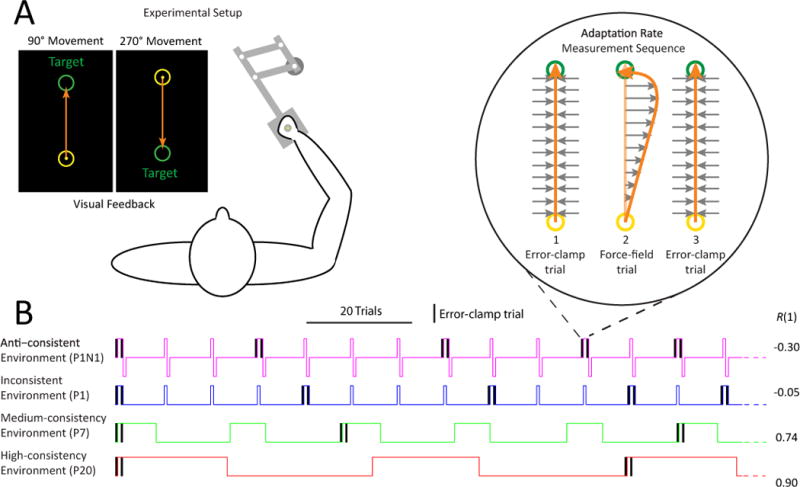
(A) Schematic of experimental setup. Subjects gripped the handle of a 2D robotic manipulandum and performed 10cm reaching arm movements in 2 directions (90° and 270°) based on targets presented on a vertical screen in front of them.

(B) Illustration of force-field environments and adaptation rate measurement sequence. Example sections of force field activation patterns for the anti-consistent, inconsistent, medium and high consistency learning environments are shown. In a subset of the FF cycles of each environment, we introduced error-clamp trials before and after the first force-field trial of the cycle (vertical black bars and blowout area). The adaptation rate was calculated as the difference in force field compensation between the post and pre force field error-clamp trials (see Equation 1). The statistical consistency, R(1), of each environment is shown on the right.

In the anti-consistent environment (P1N1) a single positive FF trial (P1) was followed by a single negative FF trial (N1) and then by 11–13 washout (null) trials. Here the positive-negative subsequence leads to a negative lag-1 autocorrelation (R(1)=−0.30). In the inconsistent environment (P1), subjects experienced a single positive FF trial followed by 10–12 washout trials, leading to a near-zero autocorrelation (R(1)=−0.05). Finally, in the medium- and high-consistency environments (P7, R(1)=0.74; and P20, R(1)=0.90), subjects experienced blocks of 7 or 20 FF trials, followed by 15–18 or 28–32 washout trials, respectively. The lag-1 autocorrelation for these last two perturbation sequences is high as most perturbations predict subsequent ones, and it increases as the block length increases because the self-similarity of a sequence after a single-trial shift is higher for longer block lengths.

We designed the experiments so that we could directly compare the adaptation rates induced by each environment. To accomplish this, we estimated the single-trial adaptation rate induced by the first FF trial of each cycle by placing error-clamp (EC) measurement trials (black bars in Figure 1B) before and after the FF trial in order to determine the change in motor output associated with the FF exposure (blowout in Figure 1B) [14, 15]. We refer to this three-trial sequence as a measurement triplet and used the difference between the lateral force output recorded on the two EC trials in each measurement triplet to measure of the change in feedforward motor output induced by exposure to the intervening FF trial. This allowed us to estimate the single-trial adaptation rate identically for all environments by comparing the observed force output change to the change that would be necessary to fully compensate for the FF perturbation.

Environmental consistency can upregulate and downregulate motor adaptation rates

We found that all groups displayed similar adaptation rates on the initial FF trial (one-way ANOVA, F(3,66)=0.87, p=0.46; 0.089±0.017, mean±SEM for all groups). However, subsequent exposure to different levels of environmental consistency resulted in single-trial adaptation rates that diverged over a range of 20-fold as shown in Figure 2A. High environmental consistency resulted in increased adaptation rates, whereas low consistency resulted in decreases, as evidenced by the changes in lateral force output patterns associated with single trial adaptation in the last half of the training period for each group (Figure 2B) and adaptation rates estimated from these force output changes (Figure 2C). Correspondingly, we found that the adaptation rates were significantly different between groups in the last half of the training period (one-way ANOVA, F(3,69)=36.46, p=3.1×10⁻¹⁴). The high-consistency (P20) and medium-consistency (P7) groups both displayed significantly increased adaptation rates (0.303±0.028, p=1.5×10⁻⁸ and 0.191±0.033, p=0.0067, respectively) relative to the initial rate (0.089±0.017), with the P20 group displaying significantly faster adaptation than the P7 group (p=0.0075). In contrast, the low-consistency group (P1) displayed a small but non-significant decrease in adaptation rate (0.058±0.010, p=0.06), and the anti-consistent group (P1N1) displayed a significantly decreased adaptation rate (0.015±0.009) compared to both the initial rate (p=0.0001) and the P1 group (p=0.0014). Because we randomized the duration of the washout period, the first perturbation trial in each cycle was somewhat unpredictable, and subjects showed no evidence of the ability to take advantage of the limited predictability that was present (see Figure S2). However, the second (negative) perturbation in P1N1 is perfectly predictable since it always follows the first, making the P1N1 environment inherently more predictable than P1, albeit in a negative manner, in line with its negative environmental consistency (R(1)=−0.30). Nevertheless, we observed a near-zero adaptation rate as opposed to a negative one in the P1N1 data, suggesting that the motor system is unable to make good use of this negative predictability, at least over the time course of our training paradigm. Overall, the data demonstrate that highly-consistent environments upregulate adaptation rates by three-fold whereas anti-consistent environments downregulate adaptation rates by five-fold. Together these results indicate that, adaptation rates can be modulated by more than an order of magnitude over the course of just a few minutes by changes in environmental consistency.

Figure 2. Upregulation and downregulation of motor adaptation rates by environmental consistency.

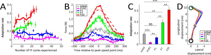
(A) Average initial adaptation rate for the P1N1, P1, P7, and P20 environments and evolution of adaptation rate in these environments as a function of the number of FF cycles experienced. Circles indicate actual data from FF cycles where the adaptation rates were measured and solid lines show a 3-point moving average. Errorbars indicate SEM across subjects.

(B) Lateral force profiles comprising the single-trial adaptive response for the different learning environments. The average learning-related change in lateral force is shown for the first cycle of the experiment averaged across experiments (gray) compared to the average FF compensation observed in the last half of the measurement FF cycles in each different environment (colors).

(C) Average initial adaptation rate for all the different learning environments (gray) compared to the last-half adaptation rates for each environment (colors). Errorbars indicate SEM. * p < 0.05, ** p < 0.01, *** p < 0.001.

(D) Average perturbed hand paths seen during the first FF trial of the experiment (gray) and in the last half of the cycles in each environment (colors). The small circles near the midway point indicate the location of the peak speed point.

Comparing next-trial adaptive responses with same-trial feedback responses

In order to determine whether the adaptation rate changes we observe are due to changes in prediction versus estimation, we compared next-trial and same-trial perturbation responses. Our hypothesis was that a change in the prediction about the persistence of perturbations from one trial to the next, would affect the next-trial adaptive response but not the same-trial feedback response. However, a change in the estimation of the size of perturbations would affect both the same-trial feedback response and the next-trial adaptive response.

An initial analysis based on data from the P1N1, P1, P7 and P20 environments yielded intriguing but inconclusive results, as detailed with statistics in the Supplemental Information. In short, we used the motor adaptation rate measured during the trial after each perturbation as a measure of next-trial response and the reduction in lateral error that was observed during the perturbation trial itself (with respect to the error observed on the very first perturbation trial) as a measure of the same-trial response – i.e. the feedback response strength. However, the results were unclear. We found that the higher-consistency environments (P7 and P20) which displayed increases in next-trial motor adaptation rates also showed increases in the strength of same-trial feedback responses. But the P7 and P20 environments also had the highest variability, obscuring whether consistency, variability, or both were responsible for the changes in same-trial and next-trial responses. Thus variability and consistency were highly correlated across these four environments (r=0.82), preventing them from being dissociated. Interestingly, next-trial responses were somewhat more tightly coupled to changes in environmental consistency (R²=0.94) than variability (R²=0.69), and same-trial responses were more tightly coupled to changes in environmental variability (R²=0.97) than consistency (R²=0.79), hinting but only hinting at a double dissociation.

Next-trial adaptive responses are driven by environmental consistency, whereas same-trial feedback responses are driven by environmental variability

To clearly dissociate the effects of environmental consistency and variability on adaptation rate and feedback response strength, we designed two new environments to have high variability but low consistency. In the first, termed “random noise” (RN), the force-field was randomly varied from one trial to the next (see Figure 3A). The second environment, P1-Long (P1L), was similar to P1 but with 2–4 rather than 10–12 null washout trials between the isolated FF trials in order to increase their frequency and thus increase environmental variability. RN’s variability (55.4 N²s²/m²) was greater than all the other environments, whereas its consistency was essentially zero (R(1)=0.02) due to its random nature. Similarly, P1L’s variability was high (46.6 N²s²/m²) whereas its consistency was low (R(1)=−0.45). Correspondingly, the inclusion of RN and P1L allows consistency and variability to be dissociated across the environments we studied, breaking the positive correlation between them, dropping their correlation from 0.82 to 0.38 (R² of 0.67 vs. 0.14).

Figure 3. Environmental consistency modulates next-trial motor adaptation rates but not same-trial feedback control.

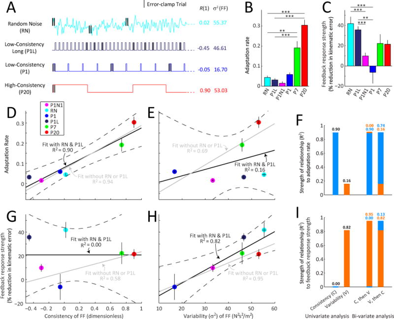
(A) Schematic of learning environments including the random noise (RN) environment. Note that the RN environment was designed to have a high variability like the high-consistency environment (P20) but at the same time a near zero consistency like the inconsistent learning environment (P1).

(B and C) Adaptation rate and feedback response strength (% reduction in kinematic error) in the last half of the P1N1, P1, RN, P7, and P20 environments. Statistical comparisons between RN and the other environments are shown (* p < 0.05, ** p < 0.01, *** p < 0.001). Errorbars indicate SEM.

(D and E) The relationships between adaptation rate and environmental consistency (D) or variability (E) across experiments. Both before (gray solid line) and after including the RN and P1L data (black solid line), environmental consistency explains a large fraction of the variance in motor adaptation rate, R2>89% in both cases. However inclusion of the RN and P1L data reduces the ability of environmental variability to explain changes in adaptation rate, reducing the R² value from 69% to only 16%. The gray dotted horizontal line indicates the initial adaptation rate before exposure to the different environments.

(G and H) The relationship between feedback response strength and environmental consistency (G) or variability (H) across experiments in a format similar to panels D and E. Both before and after including the RN data, environmental variability explains a large fraction of the variance in feedback response strength, R²=82% when including the RN/P1L data and R²=95% without. However inclusion of the RN/P1L data reduces the ability of environmental consistency to explain changes in feedback response strength, reducing the R² value from 58% to 0%. Errorbars indicate SEM.

(F and I) Summary of the strength of the relationships (R2) between adaptation rate (F) or feedback response strength (I) and consistency or variability. The first pair of bars summarizes the univariate regression analyses shown in panel D, E, G, and H. The 3rd and 4th bars summarize the corresponding bi-variate regressions. Here the 3rd bar shows the improvement in R² when a univariate analysis based on consistency (C, blue) is augmented by variability (V, orange). The 4th bar shows the improvement when a univariate analysis based on V is augmented by C. Full results of the bivariate analysis are shown in tables S2 and S3. Errorbars indicate SEM.

If adaptation rate depends on environmental variance, the RN environment should elicit adaptation rate increases even greater than those seen in the P7 and P20 environments, and P1L should elicit adaptation rate increases similar to those seen in P7. On the other hand, if adaptation rate depends on environmental consistency, neither RN nor P1L should elicit adaptation rate increases. Correspondingly, the feedback response strength elicited by the P1L and RN environments should be high if it depends on environmental variability, but low if it depends on consistency.

We found that despite substantially increased variability (55.4 vs. 16.7 N²s²/m² for RN vs. P1 and 46.6 vs. 33.2 N²s²/m² for P1L vs. P1N1, see Figure 3B,D–E), the RN and P1L environments elicited low adaptation rates, like P1 and P1N1 (0.044±0.008 vs 0.058±0.010, p=0.86 for RN vs. P1, and 0.031±0.008 vs 0.015±0.009, p=0.09 for P1L vs. P1N1). However, this is in line with similar consistency (0.02 vs. −0.05 for RN vs. P1 and −0.45 vs. −0.30 for P1L vs. P1N1). In contrast, the RN and P1L environments displayed significantly lower adaptation rates (p<0.001 for all pairwise comparisons) than both the P7 and P20 environments (0.191±0.033 and 0.303±0.028) in accordance with substantially lower consistency (0.02 and −0.45 for RN and P1L vs. 0.74 and 0.90 for P7 and P20) despite similar variability (55.4 and 46.6 vs. 45.9 and 53.0 N²s²/m²). These results provide compelling evidence for the idea that environmental consistency rather than variability determines adaptation rates. Correspondingly, the R² value for the relationship between adaptation rate and environmental consistency remains essentially unchanged at 90% when the RN and P1L data are included (F(1,4)=35.32, p=0.004, see Figure 3D), with similar results observed when considering the consistency of the kinematic error rather than the consistency of the FF environment (see Figure S3). However, the R² value between adaptation rate and variability drops precipitously from 69% to 16% (F(1,4)=0.76, p=0.43) when we include the RN and P1L experiment data as illustrated in Figure 3E. Moreover, a bivariate regression of consistency and variability onto adaptation rate reveals a significant effect of consistency but not variability (F(1,3)=22.3, p=0.018 for consistency, and F(1,3)=0.068, p=0.81 for variability). This bivariate regression accounts for 90% of the variance in the full data set, 0% improvement over consistency alone, but a 74% improvement over variability alone as shown in Figure 3F. See Table S2 of the Supplemental Information for the regression coefficients and additional detail.

When we instead examined changes in feedback response strength, we found that RN and P1L elicited levels (41.8%±6.7% and 35.7%±3.4%) that were far greater than P1 and P1N1 (−6.3%±11.0% and 9.8%±3.2%, p<0.0015 for all pairwise comparisons see Figure 3C,G–H), and more like those observed in the P7 and P20 environments (22.2%±9.1% and 21.5%±4.1%). This is in line with levels of environmental variability in RN and P1L (55.4 and 46.6 N²s²/m²) substantially higher than in P1 and P1N1 (16.7 and 33.3 N²s²/m²) but similar to P7 and P20 (45.9 and 53.0 N²s²/m²). However, this result is at odds with similar consistency for RN and P1 (0.02 vs. −0.05) and for P1L and P1N1 (−0.45 vs. −0.30) but reduced consistency for RN and P1L compared to P7 and P20 (0.02 and −0.45 vs. +0.74 and +0.90), suggesting that, unlike next-trial adaptation, same-trial feedback response strength depends on environmental variability rather than consistency. Correspondingly, the R² value for the relationship between feedback response strength and environmental variability remains high at 82% when the RN and P1L data are included (F(1,4)=17.88, p=0.013, see Figure 3H). However, the R² value between feedback response strength and environmental consistency drops sharply from 58% to 0% (F(1,4)=0.00, p=0.99) when we include the RN and P1L data, as illustrated in Figure 3G. Moreover, a bivariate regression of consistency and variability onto feedback response strength reveals a significant effect of variability but not of consistency (F(1,3)=59.03, p=0.0046 for variability, and F(1,3)=8.34, p=0.063 for consistency). This bivariate regression accounts for 95% of the variance in the full data set, 95% improvement over consistency alone, but only a 13% improvement over variability alone as shown in Figure 3I. See Table S3 of the Supplemental Information for the regression coefficients and additional detail.

Taken together, these findings indicate a striking double dissociation, with motor adaptation rate determined by environmental consistency rather than variability, but feedback response strength determined by environmental variability rather than consistency (Figure 3F,I). This finding is in line with a recent study by Yousif and Diedrichsen [16] showing that adaptive changes in feedback responses could be observed in both consistent and inconsistent environments, whereas changes in feedforward adaptation were only present in consistent environments. The positive relationship between environmental variability and feedback response strength is in line with several previous studies [17–21] and consistent with the idea that the variance of an environment informs the variance of the prior for Bayesian integration [22–25]. Moreover, the extremely tight coupling we find between feedback response strength and environmental variability indicates that the weak relationships we observe (1) between feedback response strength and environmental consistency and (2) between feedforward adaptation rate and environmental variability cannot simply result from the imprecise or noisy characterization of feedback response strength or environmental variability. The specific effect of environmental consistency on adaptation rate suggests that consistency drives changes in the motor system’s predictions about the persistence of environmental perturbations from one trial to the next which would affect next-trial adaptation, without driving changes in the motor system’s estimation of perturbation size which would affect same-trial feedback responses.

Increases in motor adaptation rate are not explained by the amount of environmental exposure

We next examined whether the improved adaptation levels we observed could be attributed to savings, which refers to the faster relearning of a previously learned task [10, 26–29]. Although our P7 and P20 experiments repeatedly trained the same FF, the durations of individual FF blocks were rather short (20 trials at most) compared to the paradigms in which savings has been demonstrated for motor adaptation [13, 26, 29], and the partial adaptation achieved in our experiments due to the relatively short FF exposures, precludes the reinforcement of successful performance that has be suggested to be a key ingredient for the instantiation of savings [13]. In fact, subjects only learn 50–70% of the force field by the last trial of the training blocks in the P7 and P20 environments where adaptation rate increases were observed (see Figure 4C). Correspondingly, we thought it unlikely that savings could be responsible for the faster adaptation observed in the P7 and P20 experiments. Nevertheless, we investigated two experimental manipulations to carefully examine the possibility.

Figure 4. Upregulation of adaptation rates cannot be explained by savings.

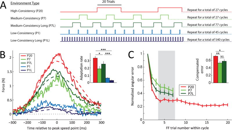
(A) Comparison of the P20 (red), P7 (light green), P7 Long (dark green), P1 (light blue) and P1L (dark blue) environments. Notice that although the number of FF cycles is the same (27) for both the P20 and P7 learning environments, the number of FF trials experienced is different, 540 vs. 189. Correspondingly, the number of FF cycles for the P1 learning environment is 45 (i.e. only 45 FF trials). The P7-Long (P7L) and P1-Long (P1L) environments were designed to match the number of FF trials of the P20 environment (540), and hence assess the influence of the number of FF trials on the observed adaptation rate increases.

(B) Lateral force profiles comprising the single-trial adaptive response in the P20, P7, P7L, P1 and P1L environments. Note that the subjects in the P7L environment, despite experiencing the same number of FF trials as those in the P20 environment, compensated less than those exposed to the P20 environment. Subjects exposed to the P1L environment compensated even less. The inset shows the average adaptation rates in the P20, P7, P7L, P1 and P1L experiments in the last third of each environment. Errorbars indicate SEM. Notice that subjects in the P20 environment exhibited adaptation rates that were significantly greater than those of subjects in all other environments.

(C) Mean angular error, a second measure of motor adaptation, in late FF cycles in the P20, P7 and P7L environments. The error in trials 4, 5, 6 and 7 (gray shaded region) of the FF cycles was significantly lower in the P20 environment than P7 or P7L. The inset quantifies these differences. Errorbars indicate SEM. * p < 0.05, ** p < 0.01, *** p < 0.001.

Because the amount of savings should depend on the amount of training, we examined whether the total duration of the exposure to the FF environment could explain the observed increases in adaptation rates as would be predicted by a savings mechanism. This possibility is compatible with the finding that the P20 environment elicited the largest adaptation rates because P20 exposed subjects to a greater number of FF trials than subjects in the other groups. This was the case because the P1 and P7 experiments were designed to match or exceed the P20 experiment in the number of cycles (45, 27, and 27, respectively) rather than FF trials (45, 189, and 540, respectively). We thus examined versions of the medium-consistency and low-consistency environment experiments, P7-Long (P7L) and P1-Long (P1L), that were lengthened in order to match the number of FF trials experienced in the P20 environment (540). We increased the number of cycles from 27 to 77 for the P7L environment and from 45 to 540 for the P1L environment, reducing the number of washout trials somewhat to avoid experiment durations greater than 4 hours (see Figure 4A and Experimental Procedures).

The P1L and P7L environments both displayed significantly lower adaptation rates than P20 (0.030±0.009 and 0.252±0.038 vs. 0.333±0.027; mean±SEM for the last third of trials for P1L, P7L and P20, respectively, p<10⁻⁸ and p=0.046 for comparisons against P20). P1L also showed a reduced adaptation rate compared to P1 (0.030±0.009 vs. 0.062±0.010, p=0.011), in line with even lower environmental consistency (R(1) of −0.45 for the P1L vs. R(1) of −0.05 for the P1) but in contrast to increased training (540 cycles for P1L vs. 45 cycles for P1). The kinematic error learning curves displayed in Figure 4C provide additional evidence for increased adaptation rate in the P20 group compared to P7 and P7L. Comparison of trials 4 through 7 in these normalized learning curves (the shaded region) indicates significantly greater kinematic error reduction in the P20 group compared to P7L (p=0.011). These findings indicate that the P20 environment elicits greater adaptation rates than low- or medium-consistency environments when equated based on either the number of cycles (P20 vs. P1 or P7) or the number of trials (P20 vs. P1L or P7L). Thus the amount of exposure cannot account for the adaptation rate differences observed between the low-, medium- and high-consistency environments, as would be predicted by a savings mechanism.

Specificity of adaptation rate increases for the experienced environment dynamics

Although we found that differences in environmental consistency rather than differences in the amount of repetition explain the pattern of learning rate changes observed across different environments (see Figure 4 above), we wondered whether repeated exposure to the same dynamics might interact with environmental consistency. In particular, does the relationship between adaptation rate and environmental consistency that we observe across environments require some degree of repetition for the trained dynamics? To investigate this possibility, we began by measuring the adaptation resulting from a single exposure to a completely novel FF – a FF opposite to the one that subjects were repeatedly trained on – after training that would increase adaptation rate. Specifically, we inserted an opposite FF trial at the end of the P7L experiment (P7L-Opposite), as illustrated in Figure 5A. The idea was that only adaptation rate upregulation that was entirely independent of repetition could result in full transfer of the adaptation rate increases observed in P7L to the P7L-Opposite trial. However, we found that the adaptive response to the P7L-Opposite trial was in the same direction as the response for the previous FF exposures despite the fact that the P7L-Opposite FF was opposite in direction to these exposures (Figure 5B). Thus, the P7L-Opposite response was inappropriately directed, and if an adaptation rate was calculated from it, that rate would be significantly negative in value (p<0.001); however, one might question whether an inappropriately-directed response should be characterized by an adaptation rate. Instead, the adaptive responses elicited by P7L-Opposite trials are more in line with repetition of the adaptive responses elicited during the P7L training than transfer of the response gains associated with this training, which were oppositely directed. However, it should be noted that the amplitude of the P7L-Opposite responses falls short of those observed during P7L training (Figure 5B, 6C–D), suggesting that the P7L-Opposite responses might not be explained by repetition alone.

Figure 5. Upregulation of adaptation rates cannot be explained by savings.

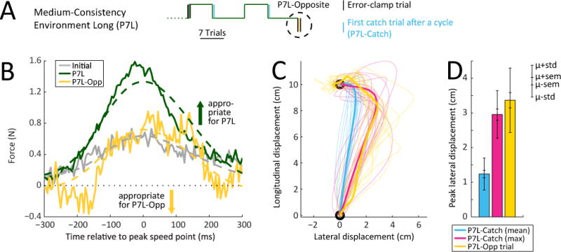
(A) Illustration of the P7L-Opposite (P7L-Opp, yellow) experiment in which a single oppositely-directed FF perturbation was presented at the end of the P7L environment. The adaptation rate for this trial was compared to the adaptation rate displayed in the last third of trials in P7L (P7L, green).

(B) Comparison of the average initial single-trial adaptive response (gray) with that observed for the last third of the P7L trials (green) and the P7L-Opposite trial (yellow). Note that in the P7L-Opposite trial, subjects produce a force compensation that is largely inappropriate for the FF experienced.

(C) Hand trajectories during the null trials immediately following FF blocks (P7L-Catch, blue: average trajectories for each subject, pink: trajectories of trials where each subject experienced their maximum deviation) compared to hand trajectories during the single P7L-Opposite trial (yellow). Thin lines indicate individual subject data; thick lines indicate data averaged across subjects. Note that the most deviated P7L-Catch trajectories are similar to the P7L-Opp ones, indicating that, while the FF experienced during the P7L-Opposite trial was completely novel, the errors it elicited were not.

(D) Peak lateral displacements / errors experienced during the P7L-Catch and P7L-Opposite trials. While on average each subject experienced weaker errors during P7L-Catch (blue), the largest P7L-Catch errors for each subject (pink) were similar to the errors experienced during P7L-Opposite. Inner errorbars indicate SEM (inner whereas outer errorbars indicate standard deviation across subjects.

Figure 6. Synergistic interaction between repetition and consistency for learning rate upregulation.

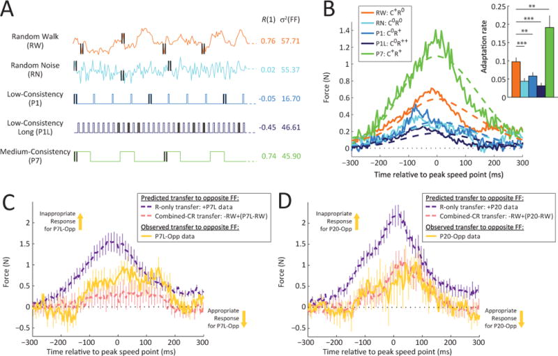
(A) Illustration of the random walk (RW) environment (orange trace). Note that this environment was designed to have a variance that is similar to that of the random noise (RN) environment (57.71 vs. 55.37), while at the same time, have a consistency similar to that of the medium-consistency (P7) environment (0.76 vs. 0.74) without having its repetitive structure.

(B) Lateral force profiles and average adaptation levels (inset) for the single-trial adaptive response in the second half of training for the RW, RN, P1, P1L and P7 environments. Note that while the force compensation in the RW environment (orange) is greater than that in the low consistency environments (RN, P1, P1L) – p<0.01 in all cases – indicating that consistency, even without repetition, leads to higher adaptation rates. However, the learning in RW does not reach the level of that in P7 (p<0.01), indicating that repetition can enhance consistency-modulated learning rate increases. Errorbars indicate SEM. * p<0.05, ** p<0.01, *** p<0.001.

(C) Repetition and consistency-driven responses combine to produce the observed P7L-Opposite response. A response predicted by the hypothesis that both consistency and repetition contribute distinct components to the adaptation (combined-CR transfer, pink dashed curve) matches the P7L-Opposite response (yellow curve) much better than a response predicted by the hypothesis that consistency enables repetition-based learning (R-only transfer, purple dashed curve). Errorbars indicate SEM.

(D) Same as (C) but for the P20 experiment, illustrating how the P20-Opposite response matches the combined-CR hypothesis rather than the R-only hypothesis.

We next examined whether the inappropriately-directed P7L-Opposite responses were associated with the novelty of the experienced dynamics or of the associated motor errors. By design, the experienced dynamics were completely novel, opposite of the only FF previously experienced. In contrast, motor errors with the same direction as the ones experienced during the P7L-Opposite trial would be expected during at the beginning of the washout period following each FF block. However, because subjects do not fully adapt by the end of each block (Figure 4C) the amplitude of the error on the first trial of washout (W1) might be substantially smaller than that experienced during the P7L-Opposite trials. Indeed, we found that the mean W1 trajectory for each participant displayed motor errors that were aligned with, but 63% smaller than the errors experienced during the P7L-Opposite trials (blue vs. yellow in Figure 5C–D, with no cases in which mean W1 errors were within 40% of the P7L-Opposite errors). However, W1 trials displayed variable trajectories from one block to the next even within the same individual, and it turns out that the upper limit of this variability (measured as the maximally displaced W1 trial for each individual during the last third of P7L exposure) is largely indistinguishable (8.9% smaller, on average) from the P7L-Opposite motor errors (pink vs. yellow in Figure 5D–E, with 83% of cases in which maximum W1 errors were within 25% of the P7L-Opposite errors or higher). Thus, whereas the experienced dynamics during P7L-Opposite were completely novel, the motor errors that participants experienced were similar to errors sometimes experienced at the beginning of each washout block. However, the adaptive response following the maximally displaced W1 trials reduced, rather than increased, the subsequent displacement for all individuals in the P7L experiment, reflecting positive rather than negative adaptation rates for the W1 trials. Thus, the inappropriately-directed P7L-Opposite response cannot be attributed to the motor errors elicited on these trials, and must instead be related to the novel dynamics experienced or the combination of the novel dynamics and the motor errors.

Repetition contributes to, but is not required for consistency-driven adaptation rate upregulation

The adaptation rate reductions observed in the P1L environment compared to P1 or to baseline indicate that repetition without consistency does not increase learning rates. However, the finding that P7L-Opposite responses reflect repetition following exposure to an environment in which repetition and consistency are combined, raises the possibility that repetition might be required for the learning rate increases observed in high-consistency environments. Thus we tested whether learning rate upregulation can occur in a high-consistency environment without repetitious exposure to specific dynamics. In particular, we studied an environment based on a damped random walk (RW) where dynamics randomly varied without repetition from one trial to the next not around zero (as in RN) but around a fixed fraction of the previous trial’s dynamics (see Supplementary Experimental Procedures). This resulted in a slowly drifting pattern (see Figure 6A) which we parameterized so that consistency (R(1)=0.76) was similar to P7 (R(1)=0.74) but much higher than RN (R(1)=0.02); however, variability (57.7 N²s²/m²) was approximately matched to both RN (55.4 N²s²/m²) and P7 (45.9 N²s²/m²).

We found that the RW environment elicited adaptation rates (0.097±0.012) that were significantly higher than RN (p=0.0004) and the other low-consistency environments, P1 (p=0.0079) and P1L (p=0.00003) as shown in Figure 6B, in line with its higher consistency. However its adaptation rate was significantly lower than that observed in P7 (p=0.0094), where a similar consistency was combined with repetition. These findings indicate that environmental consistency alone can elicit learning rate increases; however, when combined with repetition, even greater increases occur.

To examine the mechanism by which consistency and repetition combine in the P7 environment, we can re-examine the P7L-Opposite data in light of the RW results. Here, we consider three possibilities: first, that repetition enables consistency-based learning (C-only hypothesis); second, that consistency enables repetition-based learning (R-only hypothesis); and third, that both consistency and repetition contribute distinct components to the adaptation (combined CR hypothesis). The P7L-Opposite data provide a unique opportunity for examining these hypotheses because consistency-based gain modulations and repetition of the previously learned adaptive responses make opposite predictions, and these predictions can be made without reference to the P7L-Opposite data themselves – instead, deriving the R-only prediction from P7L, and the C-only prediction from RW, and the combined CR prediction from a combination of the two. We can reject the C-only hypothesis, that repetition further enables pure consistency-based learning, because consistency-based adaptation rate transfer to the P7L-Opposite trial would predict an appropriately directed response, which is opposite to what we observe. The R-only hypothesis, that high consistency enables pure repetition-based learning, correctly predicts an inappropriately directed response for P7L-Opposite; however, the amplitude of the predicted response (Figure 6C, purple) is considerably larger than the P7L-Opposite data (yellow). In contrast, the combined CR hypothesis, where both consistency and repetition contribute distinct components to the adaptation, appears to explain both the amplitude and direction of the P7L-Opposite response. Here, a flipped version of the RW data (-RW) data provides an estimate of how the consistency-based component of learning should transfer to P7L-Opposite, whereas the difference between the P7L and the RW data (P7L-RW) provides an estimate of the repetition-based component of learning. Figure 6C shows that the prediction generated from combining these components (-RW+(P7L-RW); pink) closely explains the P7L-Opposite data, matching these data more closely than the R-only and C-only predictions would. However, it should be noted that, although certainly closer to the combined-CR prediction, the P7L-Opposite data fall in between the R-only and combined-CR predictions, suggesting that this analysis might not be definitive. Thus, to further examine the issue, we examined opposite-FF responses in a group of 16 subjects who experienced a single opposite-FF trial following exposure to the P20 environment. These P20-Opposite data (Figure 6D) also match the prediction of the combined CR hypothesis considerably better than the R-only or C-only predictions. Taken together, these data suggest that environments which combine repetition and consistency, elicit a combination of consistency-based and repetition-based adaptation. In the P7 and P20 environments these contributions act in synergy; however in the P7L-Opposite and P20-Opposite data these contributions act in opposition.

Discussion

We find that experimental manipulation of environmental consistency allows for adaptation rate modulation that spans over an order of magnitude (20×), with highly-consistent environments, in which external disturbances tend to persist from one trial to the next, inducing greater than 3-fold increases in learning rate, and anti-consistent environments, in which these disturbances fluctuate in a negatively correlated manner, inducing 5-fold decreases in learning rate. Moreover, we find that whereas environmental variability determines feedback response strength but not motor adaptation rate, environmental consistency determines motor adaptation rate but not feedback response strength. This striking double dissociation gives insight into the specificity of mechanisms for same-trial control versus next-trial adaptation. However, consistency can be achieved through repetition, and the somewhat surprising results of the P7L-Opposite experiment suggested a key role for repetition in the adaptive responses we observed. Thus we closely examined the interactions between consistency and repetition. We find that even in the absence of repetition, increased consistency elicits highly significant increases in learning (RN vs. RW), however in the absence of consistency, increased repetition fails to elicit increased learning (RN vs. P1 vs. P1L), suggesting that consistency rather than repetition is primarily responsible for the learning rate increases we observe. However, we find that consistency-modulated learning rate increases are greatly magnified when repetition is combined with increased environmental consistency, indicating a strong synergistic effect between repetition and consistency.

The idea that the consistency of the environment modulates the rate of motor adaptation is in line with the idea that forming a prediction of the degree to which environmental change should persist from trial to trial is a critical step in determining the rate of adaptation. In a low-consistency or anti-consistent environment the motor system would benefit from a low adaptation rate in order to avoid overlearning from current disturbances that do not positively predict future disturbances. However, in a highly consistent environment, the motor system would benefit from rapid adaptation because disturbances experienced on one trial would be highly predictive of future disturbances. Our results show that the motor system adjusts its rate of adaptation in a way that is consistent with these ideas.

Interactions between environmental consistency and repetition

Our results reveal a surprising synergy between consistency and repetition in the learning environment. The initial set of experiments, which employed a blocked design in which a single amplitude FF alternated with a null environment (P1N1, P1, P7, and P20), demonstrated large increases in adaptation rate as consistency increased. However, the increased number of FF trials in each block resulted in increased repetition of the FF in the higher consistency environments where the block length was increased (45 vs. 189 vs. 540 FF trial repetitions for the P1, P7 and P20 experiments, respectively). We thus performed the P1L and P7L experiments (540 FF trials each) to determine whether the additional repetition present in the P20 experiment was responsible for the increased adaptation rate it elicited. But in both cases the adaptation rates were smaller than the P20 environment (p<0.0001 for P1L, and p=0.046 for P7L) and not larger than the corresponding environments with less repetition (P1L actually shows a lower learning rate than P1, p=0.011, P7L is not different than P7, p = 0.22). This, suggests that the extremely high learning rate observed in P20 was due to its increased environmental consistency, rather than increased repetition relative to the original P1 and P7 environments, and that increased repetition alone does not improve learning rates, especially when consistency is low (P1 vs P1L). To further study the effect of repetition, we created two environments (RW and RN) in which the amplitude of the FF was randomly varied over a continuous spectrum so that, strictly speaking, no repetition was present except in the probe trials themselves. This allowed us to examine the effect of environmental consistency in the absence of repetition. Here we found that the high-consistency (R(1)=0.76, similar to P7), zero-repetition RW environment elicited an adaptation rate that was significantly greater (p=0.0004) than observed in the low consistency (R(1)=0.02) zero-repetition RN environment, as shown in Figure 6. However, the adaptation rate observed for RW was significantly lower (p=0.009) than for the P7 environment, which it was matched in consistency, suggesting that the combination of consistency and repetition leads to faster learning than consistency alone.

Together, our results show that increased environmental consistency improves adaptation rates, both when repetition is low (RW vs. RN) and when repetition is high (P20 vs. P7L, and P7L vs. P1L). In contrast, increased repetition fails to increase adaptation rates when consistency is low (P1 vs. RN, and P1L vs. P1), but increased repetition does increase adaptation rates when consistency is high (P7 or P7L vs. RW). The substantial effect of repetition when consistency is high is in line with the inappropriately-directed learning we observe on the P7L-Opposite trial at the end of the P7L experiment, suggesting that repetition may lead to a stereotypic adaptive response when a large error is encountered independent of its direction. This is in line with the idea that repetition-enabled recall of actions can lead to savings in motor adaptation [13]. In summary, we find that both consistency and repetition play a role in the modulation of adaptation rates. We show that repetition alone does not lead to an increase in adaptation rate, but consistency alone does lead to an increase in adaptation rate; however, together they lead to an increase in adaptation rate that is about double that elicited by consistency alone, indicating a synergistic effect between these two key features of the learning environment.

One interpretation of these results (the C-only hypothesis) is that the primary effect that consistency has on adaptation rate is potentiated by repetition. A very different, interpretation (R-only) is that the primary effect that repetition has on adaptation rate is inhibited at low levels of environmental consistency. A third possibility (combined-CR) is that repetition and consistency contribute distinct components to the adaptive response, but that the repetition-based component requires consistency. Interestingly, we show that these interpretations make distinct predictions for the P7L-Opposite and P20-Opposite data. Of particular interest is that the combined-CR hypothesis predicts responses that sum contributions from appropriately-directed consistency-driven rate increases and inappropriately-directed repetition-enabled recall. In contrast, the R-only hypothesis predicts responses for the P7L-Opposite and P20-Opposite data that would be identical to the responses in the P7L and P20 environments. We find that the predictions of the combined-CR model match both the P7L-Opposite and P20-Opposite data better than the R-only model, suggesting that adaptive responses are characterized by an additive combination of consistency-driven learning rate increases and repetition-enabled recall; however additional work may be needed to definitively answer this important question.

Attempts to manipulate measurement noise and state noise to alter adaptation rates

Previous studies that have investigated the modulation of motor adaptation rates have focused on the estimation of the identity of the experienced perturbations [1, 2, 5]. Theoretically this estimation should be based on the appropriate weighting of the uncertainty about the state of the environment (state noise, i.e. variance on the prior expectation) relative to uncertainty about the fidelity of sensory information (measurement noise, i.e. variance on the likelihood).

According to optimal Bayesian estimation, the gain on the sensory information should be decreased when the measurement noise rises, and it should increase when the state noise rises [1, 2, 5, 23]. Correspondingly, studies have attempted to manipulate state noise and measurement noise in order to modulate the rate of adaptation [1, 2, 5]; however, these manipulations have not yielded consistent results. One set of approaches for manipulating state and measurement noise has involved perturbing the visual feedback about hand position, with a sequence that varied from one trial to the next either as white noise or a random walk [1, 2]. Here the idea was that measurement noise should be independent from one trial to the next like white noise, whereas state noise should accumulate like a random walk, and that the sensorimotor system would leverage this dichotomy by parsing the trial-to-trial variability in sensory information into independent and accumulating components to estimate the levels of measurement noise and state noise. However, there is no compelling reason to believe that this occurs. Instead, we suggest that the sensorimotor system’s estimate of measurement noise should be affected by the quality of the sensory feedback rather than its pattern across trials. For example, when a child tracks the motion of a firefly at night, she can clearly identify the location of each flash, despite having little idea where each would appear. Thus, the random pattern of flashes does not indicate high measurement noise. Only a blurred view of a flash would introduce uncertainty about the firefly’s current location. Correspondingly, experiments using white noise perturbations to randomize perturbations in an attempt to manipulate the sensorimotor system’s estimate of measurement noise have consistently failed to show the decreases in adaptation rate they predicted [1, 2]. In contrast, when studies have attempted to increase the motor system’s estimate of measurement noise by degrading the intrinsic quality of visual feedback, decreases in adaptation rate have been consistently observed [2, 5].

Moreover, studies of sensorimotor integration for same-trial feedback responses have convincingly showed that a white noise perturbation sequence leads to Bayesian integration in which state noise (the prior) rather than measurement noise (the likelihood) is increased by the perturbation variance [22–25, 30]. In fact, state noise has been taken to fully reflect the variance of the perturbation sequence in these studies. This leaves us with the conclusion that the motor system does not parse trial-to-trial variability in sensory feedback into independent and accumulating components to differentially estimate the levels of measurement noise and state noise, instead taking the entire variability as an estimate of state noise.

But then, how can we explain that studies have found accumulating random walk perturbations to result in faster adaptation rates than white noise perturbations [1, 2]? A key observation is the fact that random walk perturbations display a lag-1 autocorrelation that approaches 1 for long duration exposures and are thus, in our parlance, highly-consistent, whereas white noise perturbations display a low-consistency near zero lag-1 autocorrelation. Therefore, changes in environmental consistency can provide a unifying explanation for the current set of results and for increases in adaptation rates previously observed with random walk perturbations. This interpretation is also in line with the finding that in dynamic environments where the spatial complexity is likely to exceed the width of the basis elements for adaptation, learning rates are consistently reduced [31], as high spatial complexity could make an environment appear inconsistent.

Implications for retention of motor memories

The idea that forming a prediction of the degree to which environmental change should persist from trial to trial is a critical step in determining the rate of adaptation, also has implications for the retention of motor memories. The basic trial-to-trial learning rules presented in the introduction (see the last two equations) suggest that when error feedback is withheld, retention of the current memory will, like the learning rate, depend on the prediction factor, A. Thus the current results predict that consistency-modulated increases and decreases in learning will be accompanied, respectively, by increases and decreases in retention, i.e. decreases and increases in decay. Future work will investigate this idea.

Implications for rehabilitation

The findings described in the present study may enable the design of more effective rehabilitation protocols for stroke patients. The first four weeks post-stroke is the time window during which rehabilitation has the greatest impact on the functional recovery of patients [32–34]. Therefore, an intervention that improves the rate of motor learning during this initial period may help patients achieve better functional recovery, possibly via the design of motor rehabilitation paradigms that upregulate motor learning with high-consistency environments.

Experimental Procedures

Subjects performed 10cm point-to-point reaching movements in the 90º and 270º directions in the horizontal plane with their dominant hands while grasping the handle of a 2-link robotic manipulandum. (Figure 1A). Subjects first performed 200 movements to obtain familiarity with the task. Afterwards, in certain movements, the subjects’ trajectories were disrupted by velocity-dependent curl force-fields (FFs). We assessed the level of adaptation using error-clamp (EC) trials (i.e., we measured the force pattern that subjects produced when their lateral errors were held to near zero values in an error-clamp) [10, 35–38]. Adaptation rates were calculated by obtaining the difference between the adaptation coefficient (x) [10, 35–38] for the EC trial following the first FF trial in a measurement cycle (EC_Post) and the adaptation coefficient for the EC trial preceding this force-field trial (EC_Pre):

$$\mathit{\text{Adaptation Rate}}=x({\mathit{EC}}_{\mathit{Post}})-x({\mathit{EC}}_{\mathit{Pre}})$$ (1)

Learning environments with different levels of consistency (operationally defined as the lag-1 autocorrelation (R(1)) of the environment) and variability were created to study the environmental modulation of adaptation rate.

$$\mathit{\text{Consistency}}:R(1)=E[({\mathit{FF}}_n-{\mu }_{\mathit{FF}})({\mathit{FF}}_{n+1}-{\mu }_{\mathit{FF}})]/{\sigma }_{\mathit{FF}}^2$$ (2)

In the anti-consistent environment (P1N1; R(1)=−0.3), 21 subjects experienced to 50 cycles each with a single positive FF trial, followed by a single negative FF trial, followed by 11–13 washout (null) trials. In the inconsistent environment (P1; R(1)=−0.05), 12 subjects experienced 45 cycles with a single positive FF trial, followed by 10–12 washout trials. In the medium-consistency environment (P7; R(1)=0.74), 12 subjects experienced 27 cycles with 7 positive FF trials, followed by 15–18 washout trials. In the high-consistency environment (P20; R(1)=0.90), 28 subjects experienced 27 cycles with 20 positive FF trials, followed by 28–32 washout trials. Two additional groups completed extended versions of the P1 and P7 experiments modified to include the same number of FF trials used in the P20 experiment (P1L; R(1)=−0.45 and P7L; R(1)=0.73). 12 P1L subjects experienced 540 cycles with a single positive FF trial, followed by 1–3 washout trials, and 18 P7L subjects experienced 77 cycles with seven positive FF trials, followed by 10–14 washout trials. In addition, we added a single negative FF trial, surrounded by EC trials, after the last FF cycle in P7L and in a subset of P20 (P7L- and P20-Opposite) to assess the adaptation rate associated with this novel perturbation. To assess the adaptation rate during exposure to the learning environments, we randomly interspersed EC trials before and after the positive FF trial to form measurement triplets in a subset of the FF cycles in these experiments (40%, 44%, 44%, 44%, 22%, and 45% in P1N1, P1, P7, P20, P1L, and P7L, respectively).

13 subjects experienced a random-noise environment (RN; R(1)=0.02) where the FF trials varied randomly, with magnitudes determined according to a normal distribution with standard deviation of 7.5N/(m/s). Measurement triplets consisting of a single positive or negative FF trial, with the same magnitude (15N/(m/s)) as used in the cycle experiments described above, were randomly interspersed to assess the adaptation rate following 3% of trials. Finally, 23 subjects experienced a random-walk environment (RW; R(1) = 0.76) where the FF trials followed a random walk with a carryover coefficient of 0.88 and a noise term with a standard deviation of 2.7N/(m/s). As with RN, similar measurement triplets were used to assess the adaptation rate following 4% of trials. Please refer to the Supplemental Experimental Procedures for additional detail.

Highlights.

1. The statistical consistency of the environment determines motor adaptation rate

2. The uncertainty of the environment determines feedback response strength

3. Manipulating environmental consistency can increase or decrease adaptation rates

4. Repetition potentiates the effect of consistency in increasing motor adaptation

References

- 1.Baddeley RJ, Ingram HA, Miall RC. System identification applied to a visuomotor task: Near-optimal human performance in a noisy changing task. J Neurosci. 2003;23:3066–3075. doi: 10.1523/JNEUROSCI.23-07-03066.2003. [DOI] [PMC free article] [PubMed] [Google Scholar]
- 2.Burge J, Ernst MO, Banks MS. The statistical determinants of adaptation rate in human reaching. J Vis. 2008;8:20.21–19. doi: 10.1167/8.4.20. [DOI] [PMC free article] [PubMed] [Google Scholar]
- 3.Körding KP, Tenenbaum JB, Shadmehr R. The dynamics of memory as a consequence of optimal adaptation to a changing body. Nat Neurosci. 2007;10:779–786. doi: 10.1038/nn1901. [DOI] [PMC free article] [PubMed] [Google Scholar]
- 4.Malone LA, Vasudevan EVL, Bastian AJ. Motor Adaptation Training for Faster Relearning. J Neurosci. 2011;31:15136–15143. doi: 10.1523/JNEUROSCI.1367-11.2011. [DOI] [PMC free article] [PubMed] [Google Scholar]
- 5.Wei K, Körding K. Uncertainty of feedback and state estimation determines the speed of motor adaptation. Frontiers in Computational Neuroscience. 2010;4 doi: 10.3389/fncom.2010.00011. [DOI] [PMC free article] [PubMed] [Google Scholar]
- 6.van Beers RJ. How Does Our Motor System Determine Its Learning Rate? PLoS ONE. 2012;7:e49373. doi: 10.1371/journal.pone.0049373. [DOI] [PMC free article] [PubMed] [Google Scholar]
- 7.Kalman RE. A new approach to linear filtering and prediction problems. Journal of basic Engineering. 1960;82:35–45. [Google Scholar]
- 8.Donchin O, Francis JT, Shadmehr R. Quantifying generalization from trial-by-trial behavior of adaptive systems that learn with basis functions: Theory and experiments in human motor control. J Neurosci. 2003;23:9032–9045. doi: 10.1523/JNEUROSCI.23-27-09032.2003. [DOI] [PMC free article] [PubMed] [Google Scholar]
- 9.Sing GC, Smith MA. Reduction in Learning Rates Associated with Anterograde Interference Results from Interactions between Different Timescales in Motor Adaptation. Plos Computational Biology. 2010;6 doi: 10.1371/journal.pcbi.1000893. Article No.: e1000893. [DOI] [PMC free article] [PubMed] [Google Scholar]
- 10.Smith MA, Ghazizadeh A, Shadmehr R. Interacting adaptive processes with different timescales underlie short-term motor learning. Plos Biology. 2006;4:1035–1043. doi: 10.1371/journal.pbio.0040179. [DOI] [PMC free article] [PubMed] [Google Scholar]
- 11.Smith MA, Shadmehr R. Intact ability to learn internal models of arm dynamics in Huntington’s disease but not cerebellar degeneration. J Neurophysiol. 2005;93:2809–2821. doi: 10.1152/jn.00943.2004. [DOI] [PubMed] [Google Scholar]
- 12.Thoroughman KA, Shadmehr R. Learning of action through adaptive combination of motor primitives. Nature. 2000;407:742–747. doi: 10.1038/35037588. [DOI] [PMC free article] [PubMed] [Google Scholar]
- 13.Huang Vincent S, Haith A, Mazzoni P, Krakauer John W. Rethinking Motor Learning and Savings in Adaptation Paradigms: Model-Free Memory for Successful Actions Combines with Internal Models. Neuron. 2011;70:787–801. doi: 10.1016/j.neuron.2011.04.012. [DOI] [PMC free article] [PubMed] [Google Scholar]
- 14.Sing GC, Orozco SP, Smith MA. Limb motion dictates how motor learning arises from arbitrary environmental dynamics. J Neurophysiol. 2013;109:2466–2482. doi: 10.1152/jn.00497.2011. [DOI] [PubMed] [Google Scholar]
- 15.Sing GC, Joiner WM, Nanayakkara T, Brayanov JB, Smith MA. Primitives for motor adaptation reflect correlated neural tuning to position and velocity. Neuron. 2009;64:575–589. doi: 10.1016/j.neuron.2009.10.001. [DOI] [PubMed] [Google Scholar]
- 16.Yousif N, Diedrichsen J. Structural learning in feedforward and feedback control. J Neurophysiol. 2012;108:2373–2382. doi: 10.1152/jn.00315.2012. [DOI] [PMC free article] [PubMed] [Google Scholar]
- 17.Selen LPJ, Franklin DW, Wolpert DM. Impedance Control Reduces Instability That Arises from Motor Noise. J Neurosci. 2009;29:12606–12616. doi: 10.1523/JNEUROSCI.2826-09.2009. [DOI] [PMC free article] [PubMed] [Google Scholar]
- 18.Mitrovic D, Klanke S, Osu R, Kawato M, Vijayakumar S. A Computational Model of Limb Impedance Control Based on Principles of Internal Model Uncertainty. PLoS ONE. 2010;5 doi: 10.1371/journal.pone.0013601. [DOI] [PMC free article] [PubMed] [Google Scholar]
- 19.Franklin DW, Burdet E, Peng Tee K, Osu R, Chew CM, Milner TE, Kawato M. CNS Learns Stable, Accurate, and Efficient Movements Using a Simple Algorithm. J Neurosci. 2008;28:11165–11173. doi: 10.1523/JNEUROSCI.3099-08.2008. [DOI] [PMC free article] [PubMed] [Google Scholar]
- 20.Osu R, Kamimura N, Iwasaki H, Nakano E, Harris CM, Wada Y, Kawato M. Optimal impedance control for task achievement in the presence of signal-dependent noise. J Neurophysiol. 2004;92:1199–1215. doi: 10.1152/jn.00519.2003. [DOI] [PubMed] [Google Scholar]
- 21.Takahashi CD, Scheidt RA, Reinkensmeyer DJ. Impedance Control and Internal Model Formation When Reaching in a Randomly Varying Dynamical Environment. J Neurophysiol. 2001;86:1047–1051. doi: 10.1152/jn.2001.86.2.1047. [DOI] [PubMed] [Google Scholar]
- 22.Körding KP, Ku SP, Wolpert DM. Bayesian integration in force estimation. J Neurophysiol. 2004;92:3161–3165. doi: 10.1152/jn.00275.2004. [DOI] [PubMed] [Google Scholar]
- 23.Berniker M, Voss M, Kording K. Learning Priors for Bayesian Computations in the Nervous System. PLoS ONE. 2010;5 doi: 10.1371/journal.pone.0012686. [DOI] [PMC free article] [PubMed] [Google Scholar]
- 24.Chalk M, Seitz AR, Series P. Rapidly learned stimulus expectations alter perception of motion. J Vision. 2010;10 doi: 10.1167/10.8.2. [DOI] [PubMed] [Google Scholar]
- 25.Seydell A, Knill DC, Trommershauser J. Adapting internal statistical models for interpreting visual cues to depth. J Vis. 2010;10:1.1–27. doi: 10.1167/10.4.1. [DOI] [PMC free article] [PubMed] [Google Scholar]
- 26.Kojima Y, Iwamoto Y, Yoshida K. Memory of learning facilitates saccadic adaptation in the monkey. J Neurosci. 2004;24:7531–7539. doi: 10.1523/JNEUROSCI.1741-04.2004. [DOI] [PMC free article] [PubMed] [Google Scholar]
- 27.Krakauer JW, Pine ZM, Ghilardi MF, Ghez C. Learning of visuomotor transformations for vectorial planning of reaching trajectories. J Neurosci. 2000;20:8916–8924. doi: 10.1523/JNEUROSCI.20-23-08916.2000. [DOI] [PMC free article] [PubMed] [Google Scholar]
- 28.Medina JF, Garcia KS, Mauk MD. A mechanism for savings in the cerebellum. J Neurosci. 2001;21:4081–4089. doi: 10.1523/JNEUROSCI.21-11-04081.2001. [DOI] [PMC free article] [PubMed] [Google Scholar]
- 29.Zarahn E, Weston GD, Liang J, Mazzoni P, Krakauer JW. Explaining Savings for Visuomotor Adaptation: Linear Time-Invariant State-Space Models Are Not Sufficient. J Neurophysiol. 2008;100:2537–2548. doi: 10.1152/jn.90529.2008. [DOI] [PMC free article] [PubMed] [Google Scholar]
- 30.Körding KP, Wolpert DM. Bayesian integration in sensorimotor learning. Nature. 2004;427:244–247. doi: 10.1038/nature02169. [DOI] [PubMed] [Google Scholar]
- 31.Thoroughman KA, Taylor JA. Rapid reshaping of human motor generalization. J Neurosci. 2005;25:8948–8953. doi: 10.1523/JNEUROSCI.1771-05.2005. [DOI] [PMC free article] [PubMed] [Google Scholar]
- 32.Krakauer JW. Motor learning: its relevance to stroke recovery and neurorehabilitation. Curr Opin Neurol. 2006;19:84–90. doi: 10.1097/01.wco.0000200544.29915.cc. [DOI] [PubMed] [Google Scholar]
- 33.Kwakkel G, Kollen B, Lindeman E. Understanding the pattern of functional recovery after stroke: Facts and theories. Restor Neurol Neurosci. 2004;22:281–299. [PubMed] [Google Scholar]
- 34.Kwakkel G, Kollen BJ, van der Grond J, Prevo AJH. Probability of regaining dexterity in the flaccid upper limb - Impact of severity of paresis and time since onset in acute stroke. Stroke. 2003;34:2181–2186. doi: 10.1161/01.STR.0000087172.16305.CD. [DOI] [PubMed] [Google Scholar]
- 35.Joiner WM, Smith MA. Long-Term Retention Explained by a Model of Short-Term Learning in the Adaptive Control of Reaching. J Neurophysiol. 2008;100:2948–2955. doi: 10.1152/jn.90706.2008. [DOI] [PMC free article] [PubMed] [Google Scholar]
- 36.Scheidt RA, Reinkensmeyer DJ, Conditt MA, Rymer WZ, Mussa-Ivaldi FA. Persistence of motor adaptation during constrained, multi-joint, arm movements. J Neurophysiol. 2000;84:853–862. doi: 10.1152/jn.2000.84.2.853. [DOI] [PubMed] [Google Scholar]
- 37.Gonzalez Castro LN, Monsen CB, Smith MA. The binding of learning to action in motor adaptation. PLoS Comput Biol. 2011;7:e1002052. doi: 10.1371/journal.pcbi.1002052. [DOI] [PMC free article] [PubMed] [Google Scholar]
- 38.Joiner WM, Brayanov JB, Smith MA. The training schedule affects the stability, not the magnitude, of the interlimb transfer of learned dynamics. J Neurophysiol. 2013;110:984–998. doi: 10.1152/jn.01072.2012. [DOI] [PMC free article] [PubMed] [Google Scholar]
Associated Data
This section collects any data citations, data availability statements, or supplementary materials included in this article.