Polytomy refinement for the correction of dubious duplications in gene trees

Abstract

Motivation: Large-scale methods for inferring gene trees are error-prone. Correcting gene trees for weakly supported features often results in non-binary trees, i.e. trees with polytomies, thus raising the natural question of refining such polytomies into binary trees. A feature pointing toward potential errors in gene trees are duplications that are not supported by the presence of multiple gene copies.

Results: We introduce the problem of refining polytomies in a gene tree while minimizing the number of created non-apparent duplications in the resulting tree. We show that this problem can be described as a graph-theoretical optimization problem. We provide a bounded heuristic with guaranteed optimality for well-characterized instances. We apply our algorithm to a set of ray-finned fish gene trees from the Ensembl database to illustrate its ability to correct dubious duplications.

Availability and implementation: The C++ source code for the algorithms and simulations described in the article are available at http://www-ens.iro.umontreal.ca/~lafonman/software.php.

Contact: lafonman@iro.umontreal.ca or mabrouk@iro.umontreal.ca

Supplementary information: Supplementary data are available at Bioinformatics online.

1 INTRODUCTION

With the increasing number of completely sequenced genomes, the task of identifying gene counterparts in different organisms becomes more and more important. This is usually done by clustering genes sharing significant sequence similarity, constructing gene trees and then inferring macro-evolutionary events such as duplications, losses or transfers through reconciliation with the phylogenetic tree of the considered taxa. The inference of accurate gene trees is an important step in this pipeline. While gene trees are traditionally constructed solely from sequence alignments (Guidon and Gascuel, 2003; Ronquist and Huelsenbeck, 2003; Saitou and Nei, 1987), recent methods incorporate information from species phylogenies, gene order and other genomic footprint (Akerborg et al., 2009;Boussau et al., 2013; Durand et al., 2003; Rasmussen and Kellis, 2011; Szöllosi et al., 2013; Thomas, 2010; Wapinski et al., 2007). A large number of gene tree databases are now available (Datta et al., 2009;Flicek, 2012; Huerta-Cepas et al., 2011; Mi et al., 2012; Schreiber et al., 2013).

But constructing accurate gene trees is still challenging; for example, a significant number of nodes in the Ensembl gene trees are labelled as ‘dubious’ (Flicek, 2012). In a recent study, we have been able to show that ∼30% of 6241 Ensembl gene trees for the genomes of the fishes Stickleback, Medaka, Tetraodon and Zebrafish exhibit at least one gene order inconsistency and thus are likely to be erroneous (Lafond et al., 2013). Moreover, owing to various reasons such as insufficient differentiation between gene sequences and alignment ambiguities, it is often difficult to support a single gene tree topology with high confidence. Several support measures, such as bootstrap values or Bayesian posterior probabilities, have been proposed to detect weakly supported edges. Recently, intense efforts have been put towards developing tools for gene tree correction (Berglund-Sonnhammer et al., 2006; Chaudhary et al., 2011; Chen et al., 2000; Doroftei and El-Mabrouk, 2011; Gorecki and Eulenstein, 2011a,b; Nguyen et al., 2013; Swenson et al., 2012; Wu et al., 2012). A natural approach is to remove a weakly supported edge and collapse its two incident vertices into one (Beiko and Hamilton, 2006), or to remove ‘dubious’ nodes and join resulting subtrees under a single root (Lafond et al., 2013). The resulting tree is non-binary with polytomies (multifurcating nodes) representing unresolved parts of the tree. A natural question is then to select a binary refinement of each polytomy based on appropriate criteria. This has been the purpose of a few theoretical and algorithmic studies conducted in the past years, most of them based on minimizing the mutation (i.e. duplication and loss) cost of reconciliation (Chang and Eulenstein, 2006; Lafond et al., 2012; Vernot et al., 2009; Zheng et al., 2012).

In the present article, we consider a different reconciliation criterion for refining a polytomy, which consists in minimizing the number of non-apparent duplication (NAD) nodes. A duplication node x of a gene tree (according to the reconciliation with a given species tree) is a NAD if the genome sets of its two subtrees are disjoint. In other words, the reason x is a duplication is not the presence of paralogs in the same genome, but rather an inconsistency with the species tree. Such nodes have been flagged as potential errors in different studies (Chauve and El-Mabrouk, 2009; Flicek, 2012; Scornavacca et al., 2009). In particular, they correspond to the nodes flagged as ‘dubious’ in Ensembl gene trees.

We introduce the polytomy refinement problem in Section 2, and we show in Section 3 how it reduces to a clique decomposition problem in a graph representing speciation and duplication relationships between the leaves of a polytomy. We develop a bounded heuristic in Section 4, with guaranteed optimality in well-characterized instances. In Section 5 we exhibit a general methodology, using our polytomy refinement algorithm, for correcting NAD nodes of a gene tree. We then show in Section 6 that this approach is in agreement with the observed corrections of Ensembl gene trees from one release to another.

2 THE POLYTOMY REFINEMENT PROBLEM

Phylogenies and reconciliations. A phylogeny is a rooted tree that represents the evolutionary relationships of a set of elements (such as species, genes, … ) represented by its nodes: internal nodes are ancestors, leaves are extant elements and edges represent direct descents between parents and children. We consider two kinds of phylogenies: species trees and gene trees. A species tree $\mathcal{S}$ describes the evolution of a set of related species, from a common ancestor (the root of the tree), through the mechanism of speciation. For our purpose, species are identified with genomes, and genomes are simply sets of genes. As for a gene tree, it describes the evolution of a set of genes, through the evolutionary mechanisms of speciation and duplication. Therefore, each gene g, extant or ancestral, belongs to a species denoted by s(g). The set of genes in a gene tree is called a gene family. A leaf-label corresponds to a genome in a species tree, and to a gene belonging to a genome in a gene tree.

Given a phylogeny T, we denote by l(T) the leaf-set and by V(T) the node-set of T. Given a node x of T, we denote by l(x) and call the clade of x, the leaf-set of the subtree of T rooted at x. We call an ancestor of x any node y on the path from the root of T to the parent of x. In this case we write y < x. Two nodes x, y are unrelated if none is an ancestor of the other. For a leaf subset X of T, $lc{a}_T(X)$, the lowest common ancestor (LCA) of X in T, denotes the farthest node from the root of T, which is an ancestor of all the elements of X. In this article, species trees are assumed to be binary: each internal node has two children, representing its direct descendants (see $\mathcal{S}$ in Fig. 1). For an internal node x of a binary tree, we denote by $x_{\ell }$ and x_r the two children of x.

Definition 1 —

(Reconciliation) A reconciliation between a binary gene tree G and a species tree $\mathcal{S}$ consists in mapping each internal or leaf node x of G (representing respect. an ancestral or extant gene) to the species s(x) corresponding to the LCA in of the set $\{s(l),\text{for all}l\in l(x)\}$. Every internal node x of G is labelled by an event E(x) verifying: $E(x)=$ Speciation (S) if s(x) is different from $s(x_{\ell })$ and $s(x_r)$, and $E(x)=$ Duplication otherwise.

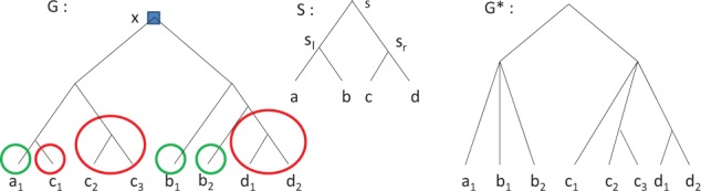
Fig. 1.

A forest $\mathcal{F}$, a species tree $\mathcal{S}$ and the corresponding graph R. Each gene tree G of $\mathcal{F}$ is attached to its corresponding node s(G) in $\mathcal{S}$. In R, joins of type AD are represented by green lines. All other lines are the joins of type S. Non-trivial AD-components (AD-components containing at least two nodes) are represented by green ovals. Red lines in R represent a vertex-disjoint clique W of R_S. Here, $R_{AD}\cup W$ has a single connected component, which leads to the binary refinement H of $\mathcal{F}$ with no NAD. After the joins of W are applied (red edges in H), the speciation-free forest can be joined with four joins AD (green vertices in H)

We define two types of duplication nodes of a gene tree G. A Non-Apparent-Duplication (NAD) is a duplication node x of G such that $\left({\cup }_{x\in l(x_{\ell })}x\right)\cap \left({\cup }_{y\in l(x_r)}y\right)=\varnothing$. A duplication that is not an NAD is an apparent duplication (AD) node, i.e. a node with the left and right subtrees sharing a common leaf-label. Therefore, any internal node x of G is of type S, AD or NAD.

The gene trees we consider might be non-binary. We call polytomy a gene tree with a non-binary root (see $\mathcal{F}$ in Fig. 1).

Definition 2 —

(Binary refinement) A tree H_T is a refinement of a tree T if and only if the two trees have the same leaf-set and T can be obtained from H_T by contracting some edges. When H_T refines T, each node of T can be mapped to a unique node of H_T so that the ancestral relationship is preserved. H_T is a binary refinement of T if and only if H_T is binary and is a refinement of T.

In this article, as only binary refinements are considered, we omit the term binary from now.

Problem statement. The general problem we address is the following: Given a non-binary gene tree G and a species tree $\mathcal{S}$, find a refinement of G containing the minimum number of NADs with respect to $\mathcal{S}$. Such a refinement of G is called a minimum refinement of G w.r.t. $\mathcal{S}$.

Hence, we aim at refining each non-binary node of G. We first show that each such non-binary node of G can be refined independently of the other non-binary nodes.

Theorem 1 —

Let $\{G_i,\text{for}1\le i\le n\}$ be the set of subtrees of G rooted at the n children $\{x_i,\text{for}1\le i\le n\}$ of the root of G. Let $H_{min}(G_i,\mathcal{S})$ be a minimum refinement of G_i w.r.t. $\mathcal{S}$. Let $G\prime$ be the tree obtained from G by replacing each G_i by $H_{min}(G_i,\mathcal{S})$. Then a minimum refinement of G is a minimum refinement of $G\prime$.

It follows from Theorem 1 that a minimum refinement of G can be obtained by a depth-first procedure iteratively solving each polytomy G_x, for each internal node x of G.

In the rest of this paper, we consider G as a polytomy, and we denote by $\mathcal{F}$ the forest $\{G_1,G_2,\dots G_n\}$ obtained from G by removing the root. For simplicity, we make no difference between a tree G_i of $\mathcal{F}$ and its root. In particular, $s(G_i)$ corresponds to $s(root(G_i))$, where $root(G_i)$ is the root of G_i (Fig. 1). We are now ready to define the main optimization problem we consider.

Minimum NAD polytomy refinement (MinNADref) problem:

Input: A polytomy G and a species tree $\mathcal{S}$;

Output: In the set $\mathcal{H}(G)$ of all refinements of G, a refinement H with the minimum number of NAD nodes. Such a refinement is called a solution to the MinNADref problem.

3 A GRAPH-THEORETICAL CHARACTERIZATION

We show (Theorem 2) that the MinNADref Problem reduces to a clique decomposition problem on a graph that represents the impact, in terms of NAD creation, of joining pairs of trees from $\mathcal{F}$.

The join graph of a polytomy. We first define a graph R based on the notion of join. A join is an unordered pair $\{G_1,G_2\}$ where $G_1,G_2\in \mathcal{F}$. The join operation j on $\{G_1,G_2\}$ consists in joining the roots of G₁ and G₂ under a common parent; we denote by $G_{1,2}$ the resulting join tree. We call the join type of $j=\{G_1,G_2\}$, and denote by $jt(G_1,G_2)$, the reconciliation label of the node created by joining G₁ and G₂ (i.e. the root of $G_{1,2}$), where $jt(G_1,G_2)\in \{S,AD,NAD\}$, respectively, for speciation, AD and NAD, w.r.t. the species tree $\mathcal{S}$.

We denote by $R=(V,E)$ the join graph of $\mathcal{F}$, defined as the unoriented complete graph on the set of vertices $V=\mathcal{F}$, where each edge (join) is labelled by the corresponding join type (Fig. 1). We denote by R_S and R_AD the subgraphs of R defined by the edges of type, respectively, S and AD. We call a connected component of R_AD an AD-component.

Let $\mathcal{F}\prime$ be the new forest obtained by replacing the two trees G₁ and G₂ of $\mathcal{F}$ by the join tree $G_{1,2}$. The rules given below, following directly from the definition of speciation and duplication in reconciliation, are used to update the join type $jt(G_{1,2},T)$ for any $T\in \mathcal{F\setminus }\{G_1,G_2\}$.

Ruleset 1

1. If $jt(G_1,T)=AD$ or $jt(G_2,T)=AD$, then $jt(G_{1,2},T)=AD$;

2. Otherwise, if $jt(G_1,T)=NAD$ or $jt(G_2,T)=NAD$, then $jt(G_{1,2},T)=NAD$;

3. Otherwise, if lca(T) is not a descendant of $lca(G_{1,2})$, then $jt(G_{1,2},T)=S$;

4. Otherwise, $jt(G_{1,2},T)=NAD$.

Clique decomposition of the join graph. Let a join sequence $J=(J_1,J_2,\dots ,J_{|J|})$ be an ordered list of joins. We denote by $\mathcal{F}(J,i)$ the forest obtained after applying the first i joins of J, starting with $\mathcal{F}$. Note that $\mathcal{F}(J,0)=\mathcal{F}$, and that $J_i\in J$ is a join on $\mathcal{F}(J,i-1)$. Let $\mathcal{J}$ denote the set of all possible join sequences of size $|\mathcal{F}|-1$. Clearly, applying all joins of a sequence $J\in \mathcal{J}$ yields a single binary tree, and there exists a gene tree $H\in \mathcal{H}(G)$ with d NADs if and only if there exists a join sequence $J\in \mathcal{J}$ with d joins of type NAD. We refine this property by showing that there is a solution to the MinNADref problem where all duplication nodes are ancestral to all speciation nodes (see the tree H of Fig. 1 for an example). The proof (not shown) makes abundant use of Ruleset 1.

Lemma 1 —

There exists a binary refinement $H\in \mathcal{H}(G)$ with d NADs if and only if there exists a join sequence $J\in \mathcal{J}$ with d joins of type NAD such that, if $J_i\in J$ is the first join not of type S in J, then all following joins J_j, for j > i, are of type AD or NAD.

We define a speciation tree as a gene tree in which every internal node is a speciation node. We deduce from the previous lemma that we can obtain a solution H to the MinNADref problem by creating a forest of speciation trees first, then successively joining them with joins of type AD or NAD. As the nodes of R corresponding to the leaves of a given speciation subtree of H are pairwise joined by speciation edges, they form a clique in R_S (in Fig. 1 the cliques in red are selected and the corresponding joins are applied to compute refinement H). The next theorem makes the link between the number of NADs of H and the cliques of R_S. For a set W of vertex-disjoint cliques of R_S, we denote by $R_{AD}\cup W$ the graph defined by the union of the edges of R_AD and W.

Theorem 2 —

A solution to the MinNADref Problem has d NADs if and only if, among all graphs $R_{AD}\cup W$ where W is a set of vertex-disjoint cliques of R_S, at least one has d + 1 connected components and none has less than d + 1 connected components.

The proof of Theorem 2 is constructive. Given an optimal set W of vertex-disjoint cliques of R_S, it leads to an optimal refinement H. Unfortunately, it can be shown that, given an arbitrary graph with two edge colours AD and S, finding if there exists a set W yielding a given number of connected components is an NP-hard problem (proof not shown). However, R is constrained by the structure of a species tree, which restricts the space of possible join graphs. An arbitrary complete graph R with edges labelled on the alphabet {S, AD, NAD} is said to be valid if there exists a species tree and a polytomy whose join graph is R. We characterize below the valid graphs in terms of forbidden induced subgraphs. The proof is partially based on well-known results on P₄-free graphs (Corneil et al. 1985).

Theorem 3 —

A graph R is valid if and only if R_S is $\{P_4,2K_2\}$-free, meaning that no four vertices of R_S induce a path of length 4, nor two vertex-disjoint edges.

Although we have not been able to find an exact polynomial-time algorithm for the MinNADref problem, this very constrained structure of the R graph yields a bounded heuristic for this problem with good theoretical properties described in the next section.

Remark 1 —

The P₄-free property, which was already introduced in relation with reconciliations in (Hellmuth et al., 2013), is of special interest, as many NP-hard problems on graphs have been shown to admit polynomial time solutions when restricted to this class of graphs. Unfortunately we can prove that, given an arbitrary P₄-free graph on which we add AD edges, finding an optimal W is still NP-hard (proof not shown). However, the added $2K_2$-free restriction imposes a rigid structure on the graph at hand, and we conjecture that there exists a polynomial time algorithm to find an optimal W.

4 A BOUNDED HEURISTIC

We first describe a general approach based on the notion of useful speciations, followed by a refinement of this approach with guaranteed optimality criteria.

Definition 3 —

Let $J=(J_1,\dots ,J_{|J|})$ be a join sequence. A join $J_i=\{G_1,G_2\}$ of J is a useful speciation if $jt(G_1,G_2)=S$ and G₁, G₂ are in two different AD-components of the R graph obtained after applying the $J_1,\dots ,J_{i-1}$ joins.

Hence, if R has c AD-components, finding a zero NAD solution becomes the problem of finding a join sequence with $c-1$ useful speciations. For example, the graph R in Figure 1 has five AD-components (three trivial and two non-trivial), and thus the four useful speciations represented by the red lines lead to a 0 NAD solution (the binary tree H). In the general case, the problem we face is to select as many useful speciations as possible, as the resulting AD-components will have to be connected by NAD joins. If we define a speciation-free forest as a forest $\mathcal{F}$ such that no edge of its join graph R is a speciation edge, following Lemma 1, we would like to first compute a set of useful speciations that results in a speciation-free forest whose join-graph has the least number of AD-components.

Definition 4 —

A lowest useful speciation is a useful speciation edge $\{G_1,G_2\}$ of R_S such that $s(G_{1,2})$ is not the ancestor of any $s(G_{i,j})$, for $\{G_i,G_j\}$ being another useful speciation edge of R_S.

Lowest useful speciations fit naturally in the context of bottom-up algorithms where speciations edges that correspond to lower vertices of $\mathcal{S}$ are selected before speciations edges corresponding to ancestral species. The theorem below shows that proceeding along these lines ensures that the resulting join sequence contains at least half of the optimal number of useful speciation.

Theorem 4 —

Let s be the maximum number of useful speciations leading to a solution to the MinNADref problem. Then any algorithm that creates a speciation-free forest through lowest useful speciations makes at least $\lceil s/2\rceil$ useful speciations.

This theorem implicitly defines a heuristic with approximation ratio 2 on the number of useful speciations that visits $\mathcal{S}$ in a bottom-up way, making useful speciations (which would thus be lowest useful speciations) whenever such an edge is available.

We now describe an improved version of this general heuristic principle. A detailed example is given in Figure 2. The main idea is to consider a bottom-up traversal of the species tree $\mathcal{S}$, and foreach visited vertex s, to find a useful set of speciation edges byfinding a matching in a bipartite graph. More precisely, foranode $s\in V(\mathcal{S})$, we consider the complete bipartite graph $\mathcal{B}=(X\cup Y,\{xy|x\in X,y\in Y\})$ such that the left (respectively right) subset X (respectively Y) contains all the trees G_i of $\mathcal{F}$where $s(G_i)$ is on the left (respectively right) subtree of s. Consider the two partitions AD_X and AD_Y of X and Y, respectively, into AD-components. The key step of our heuristic is to find a matching $M\subseteq E(\mathcal{B})$ of useful speciations between AD_X and AD_Y, called a useful matching. For example, in Figure 2, the bipartite graph and matching illustrated for Step 3 correspond to node l and that of Step 4 to node m of S.

Fig. 2.

A species tree $\mathcal{S}$ and a forest $\mathcal{F}$ of binary trees forming the polytomy. The trees of $\mathcal{F}$ are placed on $\mathcal{S}$ according to their LCA. The i, k, l and m nodes of $\mathcal{S}$ are annotated with the forest obtained after running Algorithm 2 on these nodes. Their corresponding complete bipartite matching instances are illustrated at the bottom. AD joins are represented by dotted lines, useful matching are represented by plain lines (we omit drawing all the other edges of the complete bipartite graphs). Note that there is a bridge induced by M between (F, K) and I at step 4. In the fourth step, we obtain a single connected component, which allows, in a final step, to connect all the subtrees by AD nodes (final tree is on the top of the figure)

Notice that not all edges of $\mathcal{B}$ correspond to useful speciations. Indeed it is possible that for some $x\in X$ and some $y\in Y$, although {x, y} is a speciation edge, x and y are in the same AD-component of R due to another tree z not in $\mathcal{B}$ such that {x, z} and {z, y} are AD-edges. For example in Figure 1, although $\{(a),(g)\}$ is a join of type S, the trees (a) and (g) are in the same AD-component of R due to the tree $((a,f),(g,h))$. For a vertex x of X (respectively y of Y), denote by AD(x) (respectively AD(y)) the component of AD_X (respectively AD_Y) containing x (respectively y). We indicate the fact that AD(x) and AD(y) belong to the same AD-component in R by adding two dummy genes b₁ in AD(x) and b₂ in AD(y), and a bridge $\{b_1,b_2\}$ in $E(\mathcal{B})$. Such bridges will be included in every matching, preventing to include non-useful speciation edges.

An instance P of the problem associated with a vertex s of $\mathcal{S}$ is denoted by $P=(X,Y,A{D}_X,A{D}_Y,B)$ where X, Y, AD_X, AD_Y are defined as above and B is the set of bridges induced by R. The graph corresponding to P, i.e. the complete bipartite graph on sides X and Y to which we added the bridge edges B, is denoted by $\mathcal{B}(P)$. The whole method is summarized in Algorithm 1 MinNADref($\mathcal{F},\mathcal{S}$) and illustrated on a simple example in Figure 2.

Algorithm 1: $MinNADref(\mathcal{F},\mathcal{S})$.

for each node s of $\mathcal{S}$ in a bottom-up traversal of $\mathcal{S}$ do

 Let $P=(X,Y,A{D}_X,A{D}_Y,B)$ be the problem instance corresponding to s;

 Find a useful matching M of $\mathcal{B}(P)$ of maximum size (Algorithm MaxMatching below);

 Apply each speciation of M, and update $\mathcal{F}$

end for

For each connected component C of R_AD, join the trees of C under AD Nodes;

If there is more than one tree remaining, join them under NAD nodes.

Finding a useful matching of maximum size can be done in polynomial time by Algorithm 2. For an instance $P=(X,Y,A{D}_X,A{D}_Y,B)$, the algorithm progressively increments the set M of speciation edges, eventually leading to a useful matching of maximum size. At a given step, let ${\mathcal{G}}_{P,M}$ be the graph with vertices $X\cup Y$ and edges $E_{P,M}=E_{AD}\cup M$, where E_AD is the set of AD edges of R connecting vertices of $X\cup Y$. Components $A{D}_{X_i}\in A{D}_X$ and $A{D}_{Y_j}\in A{D}_Y$ are linked if there is a path in ${\mathcal{G}}_{P,M}$ linking a vertex of $A{D}_{X_i}$ to a vertex of $A{D}_{Y_j}$, and not linked otherwise.

Algorithm 2:$MaxMatching(X,Y,X_X,A{D}_Y,B)$.

$D=\varnothing$; M = B;

while $D\ne X\cup Y$ do

 Find $C\in A{D}_X\cup A{D}_Y$ of maximum cardinality with vertices not included in D, if any; assume w.l.o.g. $C=A{D}_{X_i}\in A{D}_X$;

 for each $x\in C$ that is not incident to an edge in M do

  if there is an $y\in Y$ such that AD(y) is not linked to C then

   Find such y with AD(y) of maximum cardinality;

   Add the vertices x and y to D and add the speciation edge {x, y} to M;

  end if

 end for

 Add remaining vertices of C to D;

end while

Theorem 5 —

Given an instance $P=(X,Y,A{D}_X,A{D}_Y,B)$, Algorithm 1 finds a useful matching M of maximum size.

Algorithm 1 is a heuristic, as it may fail to give the optimal solution (refinement with minimum number of NADs), as in Figure 1 for example. In this example, a bottom-up approach would greedily speciate a and d, which cannot lead to the optimal solution. However, we prove in Theorem 6 that if transitivity holds for the duplication join type, then Algorithm 1 is an exact algorithm for the MinNADref problem. The example of Figure 1 does not satisfy this property, as $\{(a),((a,f),(g,h))\}$ is a join of duplication type (AD), $\{((a,f),(g,h)),(g)\}$ is a join of duplication type but $\{(a),(g)\}$ is a join of speciation type.

Theorem 6 —

(1) Let s be the maximum number of useful speciations leading to a solution to the MinNADref problem. Then, Algorithm 1 makes at least $\lceil s/2\rceil$ useful speciations. (2) If, for every node s of $\mathcal{S}$ the instance P corresponding to s has no bridges, then Algorithm 1 outputs a refinement of the input polytomy with the maximum number of useful speciations.

The following corollary provides an alternative formulation of the optimality result given by the above theorem.

Corollary —

Algorithm 1 exactly solves the MinNADref problem for an input $(\mathcal{F},\mathcal{S})$ such that each AD-component of the corresponding graph R is free from S edges (i.e. there is no S edge between any two vertices of a given AD-component).

5 GENE TREE CORRECTION

The polytomy refinement problem is motivated by the problem of correcting gene trees. Duplication nodes can be untrusted for many reasons, one of them being the fact that they are NADs, pointing to disagreements with the species tree that are not due to the presence of duplicated genes. Different observations tend to support the hypothesis that NAD nodes may point at erroneous parts of a gene tree (Chauve and El-Mabrouk, 2009; Swenson et al., 2012). For example, the Ensembl Compara gene trees (Vilella et al., 2009) have all their NAD nodes labelled as ‘dubious’. In (Chauve and El-Mabrouk, 2009), using simulated datasets based on the species tree of 12 Drosophila species given in (Hahn et al., 2007) and a birth-and-death process, starting from a single ancestral gene, and with different gene gain/loss rates, it has been found that 95% of gene duplications lead to an AD vertex. Although suspected to be erroneous, some NAD nodes may still be correct, due to a high number of losses. However, in the context of reconciliation, the additional damage caused by an erroneous NAD node is the fact that it significantly increases the real rearrangement cost of the tree (Swenson et al., 2012). Therefore, tools for modifying gene trees according to NADs are required. We show now how Algorithm 1 can be used in this context.

In (Lafond et al., 2013), a method for correcting untrusted duplication nodes has been developed. The correction of a duplication node x relies on pushing x by multifurcation, which transforms x into a speciation node with two children being the roots of two polytomies. Figure 3 recalls the pushing by multifurcation procedure. These polytomies are then refined by using an algorithm developed in (Lafond et al., 2012), which optimizes the mutation cost of reconciliation.

Fig. 3.

A gene tree G and a species tree $\mathcal{S}$, from which we obtain $G^{*}$ by pushing x by multifurcation. Here, x is a NAD, and is pushed by taking the forest of maximal subtrees of G that only have genes from species in the s_l subtree (green), then another forest for the s_r subtree (red) in the same manner. Both these forests are joined under a polytomy, which are then joined under a common parent, so the root of $G^{*}$ is a speciation

In the context of correcting NADs, we use the same general methodology, but now using Algorithm MinNADref for refining polytomies. Removing all NADs of a gene tree can then be done by iteratively applying the above methodology on the highest NAD node of the tree (the closest to the root).

6 RESULTS

Simulated data. Simulations are performed as follows. For a given integer n, we generate a species tree $\mathcal{S}$ with a random number of leaves between $0.5n$ and 3n. We then generate a forest $\mathcal{F}=(G_1,\dots ,G_n)$ of cherries by randomly picking, for each cherry $G_i\in \mathcal{F}$, one node $s_i\in S$ and two leaves, one from each of the two subtrees rooted at s_i. Any leaf of $\mathcal{S}$ is used at most once (possibly by adding leafs to $\mathcal{S}$ if required), leading to a set of cherries related through joins of type S or NAD. Then, for each pair $\{G_i,G_j\}$ with join type NAD, we relate them through AD with probability 1/2 (or do nothing with probability 1/2), by adding a duplicated leaf.

For each pair $(S,\mathcal{F})$, we compared the number of NADs found by Algorithm MinNADref with the minimum number of NADs returned by an exact algorithm exploring all possible binary trees that can be constructed from $\mathcal{F}$. We generated a thousand random $\mathcal{S}$ and $\mathcal{F}$ for each $n\ge 4$. We stopped at n = 14, as the brute-force algorithm is too time-costly beyond this point. Over all the explored datasets simulated as described above, Algorithm MinNADref was able to output an optimal solution, i.e. a refinement with the minimum number of NADs. Therefore, the examples on which the heuristic fails seem to be rare, and the algorithm performs well on polytomies of reasonable size.

We then wanted to assess how the NAD minimization criterion differs from the rearrangement cost minimization criterion. We generated 960 random instances with forests of sizes ranging between 5 and 100 (10 instances for each $5\le n\le 100$). We compared the output of Algorithm MinNADref with that of Algorithm MinDLref, given in (Lafond et al., 2012), which computes refinement minimizing the duplication+loss (DL) cost of reconciliation with the species tree. Both algorithms gave the exact same refinement for only 12 instances (1.25%). As expected, Algorithm MinNADref always yielded a refined tree with a lower or equal number of NADs than the tree given by Algorithm MinDLref, but always had a higher or equal DL-cost. However, in many cases, minimizing the DL-score did not minimize the number of NADs, as in 377 instances (39.3%), Algorithm MinNADref yielded strictly less NADs than Algorithm MinDLref.

Ensembl Gene Trees.

Next we tested the relevance of the proposed gene tree correction methodology, by exploring how Ensembl gene trees are corrected from one release to another. As the Ensembl general protocol for reconstructing gene trees does not change between releases, the observed modifications on gene trees are more likely due to modifications on gene sequences.

We used the Ensembl Genome Browser to collect all available gene trees containing genes from the monophyletic group of ray-finned fishes (Actinopterygii), and filtered each tree to preserve only genes from the taxa of interest (ray-finned fish genomes). We selected from both Releases 74 (the present one) and 70 the 1096 gene trees that are present in both with exactly the same set of genes from the monophyletic group of fishes, and with less NAD nodes in Release 74. We wanted to see to what extent our general principle of correcting an NAD by transforming it to a speciation node is observed by comparing Rel.70 to Rel.74. Such a transformation requires to preserve the clade of the corrected NAD node x of the initial tree, meaning that l(x) should also be the leaf-set of a subtree in the corrected tree. For >90% of these trees (993 trees), the highest NAD node clade was preserved in Rel.74. Moreover, among all such nodes that were corrected, i.e. were not NAD nodes in Rel.74 (641 trees), almost all were transformed into speciation nodes (630 trees), which strongly supports our correction paradigm.

To evaluate our methodology for correcting NADs, we applied it to the highest NAD node of each of the 1096 aforementioned trees of Rel.70. Figure 4 illustrates a comparison between the corrected trees (Rel.70C, C standing for ‘Corrected’) obtained by our methodology and those of Rel. 74. Pairwise comparisons are based on the normalized Robinson–Foulds (RF) distance (number of identical clades divided by the total number of clades). The yellow curve shows a good correlation between Rel.70C and Rel.74, with ∼65% exhibiting >80% similar clades between Rel.70C and Rel.74. If we reduce the set of trees to those for which the highest NAD node is also transformed to a speciation node in Rel.74 (630 trees), the correlation is even better (blue curve of Fig. 4), with 44% of trees being identical (277 over 630 trees) and ∼80% exhibiting >80% similar clades between Rel.70C and Rel.74. Now, to specifically evaluate Algorithm MinNADref, we further restricted the set of trees to those giving rise to a non-trivial polytomy (i.e. polytomy of degree > 2) after the pushing by multifurcation, which leads to a set of 117 trees. Overall, the results for these trees (red curve in Fig. 4) are close to those observed for all trees (yellow curve) detailed above.

Fig. 4.

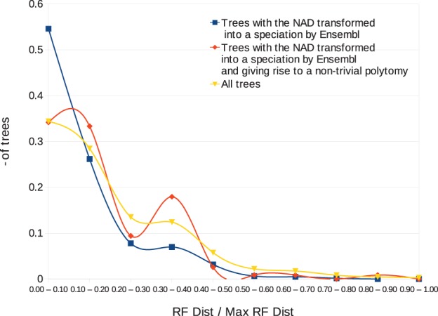
Normalized RF-distance between corrected gene trees (by modification of the highest NAD) from Rel. 70 and corresponding gene trees in Rel. 74. Blue curve: transformation of the highest NAD into a speciation. Red curve: trees with a non-trivial polytomy after pushing by multifurcation. Yellow curve: all trees

We then wanted to evaluate our correction of the 117 aforementioned trees compared with trees in Rel.74. Figure 5 provides an evaluation of the corrected trees (yellow curve) compared with those in Rel. 74 (blue curve) based on the normalized RF distance with the initial trees in Rel.70. Overall, the initial tree is closer to our correction than to the one of Rel.74. Therefore, even though gene trees of Rel.74 are likely to have stronger statistical support with respect to the gene sequences provided in Rel.74, our correction removes NADs while respecting as much as possible the given tree topology. Finally, we considered the reconciliation mutation cost as another evaluation criterion. Among the 117 trees of Rel.70C, 30 are identical to the corresponding trees in Rel. 74, and 60% have a lower mutation cost, which tend to support our correction compared with the tree in Rel.74. As for the 40% remaining trees, half of them have more NADs than the corresponding tree in Rel.74, which suggests that applying our correction to all NAD, instead of just the highest one, would help to obtain better results.

Fig. 5.

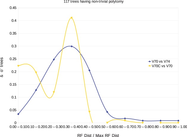
Normalized RF-distance between corrected trees (yellow curve) and Rel. 74 trees (blue curve) and original Rel. 70 trees

Finally, we evaluated the effect of NAD correction on the tree likelihood. For this purpose, we selected the 1891 Ensembl Rel.74 gene trees of the considered monophyletic group containing at least one NAD, and we corrected each NAD individually. The sequences were aligned using ClustalW (Larkin et al., 2007) and the likelihood values were computed with PhyML (Guidon et al., 2003). For a tree T and a NAD node x, denote by T_x the tree obtained after correcting x. For each T and each x, we computed the log-likelihood ratio $L(x)=logLH(T)/logLH(T_x)$. Among the 4454 NAD nodes found in the considered set of trees, 95.4% of the L(x) ratios were between 0.98 and 1.02. Although the correction algorithm is not expected to outperform the Ensembl protocol in terms of likelihood as it ignores sequences, we found that the likelihood of the tree has been improved (L(x) > 1) after correction for 43.9% of the NAD nodes. Moreover, 1180 (62.4%) trees contained at least one NAD node improving the likelihood.

7 CONCLUSION

The present work is dedicated to the polytomy refinement problem. While the mutation cost of reconciliation has been used previously as an optimization criterion for choosing an appropriate binary tree, here we use an alternative criterion, which is the minimization of NADs. The tractability of the MinNADref Problem remains open, as is the problem to select, among all possible solutions, those leading to a minimum reconciliation cost. Although developing a gene tree correction tool is not the purpose of this article, we show how our algorithm for polytomy refinement can be used in this context, by developing a simple algorithm allowing to correct a single NAD. This algorithm has been applied to trees of a previous Ensembl release, and the corrected trees have been compared with the trees of the current Ensembl release. A good correlation between the two sets of trees is observed, which tends to support our correction paradigm. While minimizing NADs cannot be a sufficient criterion for gene tree correction, it should rather be seen as one among others, such as statistical (Wu et al., 2012), syntenic (Lafond et al., 2013) or based on reconciliation with the species tree (Chaudhary et al., 2011; Lafond et al., 2013; Swenson et al., 2010), that can be integrated in a methodological framework for gene tree correction.

Funding: N.E.-M. and M.L. are supported by ‘Fonds de recherche du Québec—Nature et technologies’ (FRQNT). C.C. and N.E.-M. are supported by the Natural Sciences and Engineering Research Council of Canada (NSERC). R.D. is supported by the MIUR PRIN 2010–2011 grant ‘Automi e Linguaggi Formali: Aspetti Matematici e Applicativi’, code H41J12000190001.

Conflict of interest: none declared.

REFERENCES

- Akerborg O, et al. Simultaneous bayesian gene tree reconstruction and reconciliation analysis. Proc. Natl Acad. Sci. USA. 2009;106:5714–5719. doi: 10.1073/pnas.0806251106. [DOI] [PMC free article] [PubMed] [Google Scholar]
- Beiko RG, Hamilton N. Phylogenetic identification of lateral genetic transfer events. BMC Evol. Biol. 2006;6:15. doi: 10.1186/1471-2148-6-15. [DOI] [PMC free article] [PubMed] [Google Scholar]
- Berglund-Sonnhammer AC, et al. Liberles. Optimal gene trees from sequences and species trees using a soft interpretation of parsimony. J. Mol. Evol. 2006;63:240–250. doi: 10.1007/s00239-005-0096-1. [DOI] [PubMed] [Google Scholar]
- Boussau B, et al. Genome-scale coestimation of species and gene trees. Genome Res. 2012;23:323–330. doi: 10.1101/gr.141978.112. [DOI] [PMC free article] [PubMed] [Google Scholar]
- Chang WC, Eulenstein O. 2006. Reconciling gene trees with apparent polytomies. In: COCOON 2006. Lecture Notes in Computer Science. Vol. 4112, Springer, Taiwan, pp. 235–244. [Google Scholar]
- Chaudhary R, et al. Efficient error correction algorithms for gene tree reconciliation based on duplication, duplication and loss, and deep coalescence. BMC Bioinformatics. 2011;13(Suppl.10):S11. doi: 10.1186/1471-2105-13-S10-S11. [DOI] [PMC free article] [PubMed] [Google Scholar]
- Chauve C, El-Mabrouk N. 2009. New perspectives on gene family evolution: losses in reconciliation and a link with supertrees. RECOMB 2009. Lecture Notes in Computer Science. Vol. 5541, Springer, USA, pp. 46–58. [Google Scholar]
- Chen K, et al. Notung: dating gene duplications using gene family trees. J. Comp. Biol. 2000;7:429–447. doi: 10.1089/106652700750050871. [DOI] [PubMed] [Google Scholar]
- Corneil DG, et al. A linear recognition algorithm for cographs. SIAM J. Comput. 1985;14:926–934. [Google Scholar]
- Datta RS, et al. Berkeley phog: phylofacts orthology group prediction web server. Nucleic Acids Res. 2009;37:W84–W89. doi: 10.1093/nar/gkp373. [DOI] [PMC free article] [PubMed] [Google Scholar]
- Doroftei A, El-Mabrouk N. 2011. Removing noise from gene trees. WABI 2011. Lecture Notes in Bioinformatics. Vol. 6833, Springer, Germany, pp. 76-91. [Google Scholar]
- Durand D, et al. A hybrid micro-macroevolutionary approach to gene tree reconstruction. J. Comput. Biol. 2006;13:320–335. doi: 10.1089/cmb.2006.13.320. [DOI] [PubMed] [Google Scholar]
- Larkin MA, et al. Clustalw and clustalx version 2. Bioinformatics. 2007;23:2947–2948. doi: 10.1093/bioinformatics/btm404. [DOI] [PubMed] [Google Scholar]
- Flicek P. Ensembl 2012. Nucleic Acids Res. 2012;40:D84–D90. doi: 10.1093/nar/gkr991. [DOI] [PMC free article] [PubMed] [Google Scholar]
- Gorecki P, Eulenstein O. Algorithms: simultaneous error-correction and rooting for gene tree reconciliation and the gene duplication problem. BMC Bioinformatics. 2011a;13(Suppl. 10):S14. doi: 10.1186/1471-2105-13-S10-S14. [DOI] [PMC free article] [PubMed] [Google Scholar]
- Gorecki P, Eulenstein O. 2011b. A linear-time algorithm for error-corrected reconciliation of unrooted gene trees. ISBRA 2011. Lecture Notes in Bioinformatics. Vol. 6674, Springer, China, pp. 148–159. [Google Scholar]
- Guidon S, Gascuel O. A simple, fast and accurate algorithm to estimate large phylogenies by maximum likelihood. Syst. Biol. 2003;52:696–704. doi: 10.1080/10635150390235520. [DOI] [PubMed] [Google Scholar]
- Hahn MW, et al. Gene family evolution across 12 drosophilia genomes. PLoS Genet. 2007;3:e197. doi: 10.1371/journal.pgen.0030197. [DOI] [PMC free article] [PubMed] [Google Scholar]
- Hellmuth M, et al. Orthology relations, symbolic ultrametrics, and cographs. J. Math. Biol. 2013;66:399–420. doi: 10.1007/s00285-012-0525-x. [DOI] [PubMed] [Google Scholar]
- Huerta-Cepas J, et al. Phylomedb v3.0: an expanding repository of genome-wide collections of trees, alignments and phylogeny-based ozrthology and paralogy predictions. Nucleic Acids Res. 2011;39:D556–D560, 2011. doi: 10.1093/nar/gkq1109. [DOI] [PMC free article] [PubMed] [Google Scholar]
- Lafond M, et al. Gene tree correction guided by orthology. BMC Bioinformatics. 2012;14(Suppl. 15):S5. doi: 10.1186/1471-2105-14-S15-S5. [DOI] [PMC free article] [PubMed] [Google Scholar]
- Lafond M, et al. Error Detection and Correction of Gene Trees. 2013. Models and algorithms for genome evolution. Springer, Canada. 2013. [Google Scholar]
- Lafond M, et al. 2012. An optimal reconciliation algorithm for gene trees with polytomies. WABI 2012. Lecture Notes in Computer Science. Vol. 7534. pp. 106–122. [Google Scholar]
- Mi H, et al. Panther in 2013: modeling the evolution of gene function, and other gene attributes, in the context of phylogenetic trees. Nucleic Acids Res. 2012;41:D377–D386. doi: 10.1093/nar/gks1118. [DOI] [PMC free article] [PubMed] [Google Scholar]
- Rasmussen MD, Kellis M. A bayesian approach for fast and accurate gene tree reconstruction. Mol. Biol. Evol. 2011;28:273–290. doi: 10.1093/molbev/msq189. [DOI] [PMC free article] [PubMed] [Google Scholar]
- Ronquist F, Huelsenbeck JP. MrBayes3: Bayesian phylogenetic inference under mixed models. Bioinformatics. 2003;19:1572–1574. doi: 10.1093/bioinformatics/btg180. [DOI] [PubMed] [Google Scholar]
- Saitou N, Nei M. The neighbor-joining method: a new method for reconstructing phylogenetic trees. Mol. Biol. Evol. 1987;4:406–425. doi: 10.1093/oxfordjournals.molbev.a040454. [DOI] [PubMed] [Google Scholar]
- Schreiber F, et al. Treefam v9: a new website, more species and orthology-on-the-fly. Nucleic Acids Res. 2013;42:D922–D925. doi: 10.1093/nar/gkt1055. [DOI] [PMC free article] [PubMed] [Google Scholar]
- Scornavacca C, et al. 2009. From gene trees to species trees through a supertree approach. LATA 2009. Lecture Notes in Computer Science. Vol. 5457. pp. 702–714. [Google Scholar]
- Swenson KM, et al. Gene tree correction for reconciliation and species tree inference. Algorithms Mol. Biol. 2012;7:31. doi: 10.1186/1748-7188-7-31. [DOI] [PMC free article] [PubMed] [Google Scholar]
- Szöllosi GJ, et al. Efficient exploration of the space of reconciled gene trees. Syst. Biol. 2013;62:901–912. doi: 10.1093/sysbio/syt054. [DOI] [PMC free article] [PubMed] [Google Scholar]
- Nguyen TH, et al. Reconciliation and local gene tree rearrangement can be of mutual profit. Algorithms Mol. Biol. 2013;8:12. doi: 10.1186/1748-7188-8-12. [DOI] [PMC free article] [PubMed] [Google Scholar]
- Thomas PD. GIGA: a simple, efficient algorithm for gene tree inference in the genomic age. BMC Bioinformatics. 2010;11:312. doi: 10.1186/1471-2105-11-312. [DOI] [PMC free article] [PubMed] [Google Scholar]
- Vernot B, et al. Reconciliation with non-binary species trees. J. Comput. Biol. 2008;15:981–1006. doi: 10.1089/cmb.2008.0092. [DOI] [PMC free article] [PubMed] [Google Scholar]
- Vilella AJ, et al. EnsemblCompara genetrees: complete, duplication-aware phylogenetic trees in vertebrates. Genome Res. 2009;19:327–335. doi: 10.1101/gr.073585.107. [DOI] [PMC free article] [PubMed] [Google Scholar]
- Wapinski I, et al. Automatic genome-wide reconstruction of phylogenetic gene trees. Bioinformatics. 2007;23:i549–i558. doi: 10.1093/bioinformatics/btm193. [DOI] [PubMed] [Google Scholar]
- Wu Y-C, et al. Treefix: statistically informed gene tree error correction using species trees. Syst. Biol. 2012;62:110–120. doi: 10.1093/sysbio/sys076. [DOI] [PMC free article] [PubMed] [Google Scholar]
- Zheng Y, et al. Reconciliation of gene and species trees with polytomies. 2012 eprint arXiv:1201.3995. [Google Scholar]
Associated Data
This section collects any data citations, data availability statements, or supplementary materials included in this article.