Quantifying sequence and structural features of protein–RNA interactions

Abstract

Increasing awareness of the importance of protein–RNA interactions has motivated many approaches to predict residue-level RNA binding sites in proteins based on sequence or structural characteristics. Sequence-based predictors are usually high in sensitivity but low in specificity; conversely structure-based predictors tend to have high specificity, but lower sensitivity. Here we quantified the contribution of both sequence- and structure-based features as indicators of RNA-binding propensity using a machine-learning approach. In order to capture structural information for proteins without a known structure, we used homology modeling to extract the relevant structural features. Several novel and modified features enhanced the accuracy of residue-level RNA-binding propensity beyond what has been reported previously, including by meta-prediction servers. These features include: hidden Markov model-based evolutionary conservation, surface deformations based on the Laplacian norm formalism, and relative solvent accessibility partitioned into backbone and side chain contributions. We constructed a web server called aaRNA that implements the proposed method and demonstrate its use in identifying putative RNA binding sites.

INTRODUCTION

Many biological processes require specific interactions between protein and RNA molecules. Protein–RNA interactions coordinate the flow of genetic information from transcription to translation at various levels (1–3). Protein and RNA molecules can fold together to form stable subunits of molecular machines such as the ribosome (4) or spliceosome (5) and also form transient complexes, such as target-specific ribonucleases (6) and helicases (7). Like proteins, RNA molecules can adopt myriad structural conformations, a consequence of which is a great variety of protein–RNA interaction motifs. Understanding the underlying principles of these interactions is a non-trivial task since there are far fewer solved structures of protein–RNA complexes than there are known interactions and RNA structure determination poses a unique set of challenges (8). Nevertheless, the growth rate of structurally determined protein–nucleotide complexes has continued to rise over the last decade. Therefore, there is a need to establish methods that can reliably translate such structural data into predictive models.

Computational methods for the prediction of RNA binding sites on proteins make use of various features. A number of methods are based on sequence information, including: PiRaNhA (9), which uses position-specific scoring matrices (PSSMs), inherent binding propensities of interface residues, solvent accessibility and hydrophobicity; BindN+ (10), which uses side chain pKa, hydrophobicity, the molecular masses of residues and evolutionary information captured by PSSMs; PRBR (11), which uses predicted secondary structure, conservation of residue physicochemical properties and residue-dependent charge-polarity and hydrophobicity; SRCPred (12), which uses PSSMs and global amino acid composition (GAC) to predict di-nucleotide binding propensities. Methods that make use of structural information include: KYG (13), which combines residue-based binding propensities, spatially close residue doublets, and sequence profiles; DRNA (14), which performs alignment with known complex structures and scores targets with a statistical energy function and OPRA (15), which uses accessible-surface-weighed residue binding propensities calculated from known binding interfaces.

Sequence-based predictors are usually shortsighted, due to their fragmented view of a binding site; a sliding window can only capture a continuous segment of sequential residues, thereafter neglecting correlation between sequentially distant but spatially close residues. In contrast, structure-based predictors can reach higher specificity but usually at a cost of sensitivity (16). Structure-based methods generally attempt to recall geometric features from known protein–RNA complexes and fit these to geometric features of query proteins. Due to the large degree of freedom introduced by protein folding from 1D sequence to 3D structure and the limited number of training structures, geometric features of RNA-binding proteins have not been exhaustively explored, resulting in lower sensitivity as compared with sequence-based methods. As a consequence of these tradeoffs, we aimed to develop a method that could optimally utilize both sequence and structural features of RNA-binding proteins in order to accurately quantify their contributions to protein–RNA molecular recognition.

To this end, we have made use of several established and novel features. In addition to the sequence features used previously in the SRCPred method (12), we included hidden Markov model (HMM)-based evolutionary conservation (EC) scores to better evaluate conservation. We adopted an algorithm that collects positional amino acid occurrence from reweighed alignments acquired through HMM-based comparisons (17). We found that the HMM-based EC feature provided a more straightforward measure of EC than the previously described PSSM-based feature (12). For structural features, we made use of local relative accessible surface area, which we developed in a novel way and mapped onto patches of spatially neighboring residues in order to capture information from spatially close residues. Finally, we represented molecular structure by using the Laplacian norm (LN) (18). LN is a structural descriptor that measures surface convexity/concavity over different length scales. By tuning the granularity, the LN could be made tolerant to structural deviations among RNA binding surfaces, while still being sensitive enough to distinguish binding surfaces from non-binding ones. Consequently, both sensitivity and specificity of the predictor could be achieved.

In summary, we present an RNA binding site predictor using various features that outperforms sequence- or structure-only predictors. Importantly, the proposed method makes use of structural features even for sequence-only input through in-line homology modeling and is robust with respect to typical input noise levels that occur in the homology modeling phase. The proposed method has been implemented as a web service called aaRNA at http://sysimm.ifrec.osaka-u.ac.jp/aarna/, and is expected to enhance functional annotation of putative RNA-binding proteins at the residue level.

MATERIALS AND METHODS

Dataset and contact profile

Protein–RNA complexes with a resolution better than 3.0 Å and solved by X-ray crystallography were downloaded from the Protein Data Bank (PDB) (19) in May 2013. Only protein chains with at least 30 resolved residues and no <3 residues in RNA contact were considered. We also required the RNA partner chain or chains to be at least 3 nucleotides long. Protein chains that include only carbon alpha (Cα) atoms were discarded. Redundancy among protein chains was reduced by clustering them using BLASTCLUST at a 25% sequence identity threshold. From each protein chain cluster, we selected a representative with the largest number of RNA contacts. A protein–RNA contact was defined structurally, and only contacts between protein and RNA chains within the same biological unit (BU) were considered. For a structure with a single BU, an amino acid and ribonucleotide residue pair was considered to be in contact when their minimum distance was <3.5 Å. For structures with multiple BUs, individual units were separated following ‘REMARK 350’ records in their respective PDB files. Contacts taking place at the interface of two nearby BUs were ignored, because these interactions might not be functionally relevant. A di-nucleotide contact is defined as a nucleotide in contact together with one of its flanking nucleotides on either direction. We neglected structurally unresolved protein residues because neither contact nor structure could be defined. Protein chains were partitioned into a ‘non-ribosomal’ and a ‘full’ (ribosome-including) dataset; the former included no protein chains interacting with bulky ribosomal RNAs (longer than 200 bps), resulting in 141 and 205 protein chains, respectively. Two supplementary files listing all PDB protein and RNA chains for contact included in the dataset can be found at Supplementary Materials. In the non-ribosomal dataset, 2899 out of 43 863 residues were RNA binding, while in the full dataset, 5493 out of 51 781 residues were RNA binding. With the full dataset, we further checked hydrogen bonds in the structures using HBPLUS (20), and analyzed contact preferences between protein residues and RNA nucleotides. Note that in order to identify hydrogen bonds correctly, a profile indicating atoms of hydrogen donator and acceptor in nucleotides must be prepared. In particular, the O3’ atom of ribose can only serve as an acceptor after forming a phosphodiester bond.

Artificial neural network training and testing

Binary and di-nucleotide classifiers were built by using an artificial neural network algorithm implemented in the Stuttgart Neural Network Simulator suite (http://wolf.bms.umist.ac.uk/naccess). A three-layered fully connected network was constructed and trained via a standard back propagation protocol. The number of nodes in the first network layer equaled the number of training features (to be described below), and the last output layer contained either 1 or 16 output nodes (ranging from 0 to 1 in value) for binary and di-nucleotide classifiers, respectively. In the later case, the 16 output nodes are due to the 16 possible di-nucleotide combinations: [A|C|G|U] x [A|C|G|U]. The number of nodes in the middle hidden layer was tuned to optimize the performance, resulting in a five-node layer. The performance of the model was assessed by a five-fold cross-validation scheme. Instead of randomly sampling an equal number of ‘positive’ (i.e. RNA binding) and negative (i.e. non-binding) inputs, a more stringent method was used. A nearly equal number of protein chains (28 or 29 for the RB141 dataset and 41 for the RB205 dataset) were randomly allocated into five subsets, with each subset containing only residues from the assigned chains. Then, three out of five subsets were iteratively selected to train the network. To avoid over-fitting, training was halted when an early stopping criterion was satisfied based on evaluation by one of the subsets left out. Finally, the last remaining subset was tested by the network to estimate the performance. All protein chains were tested after shuffling training and testing datasets in this way. This approach to training and testing resulted in a far larger proportion of negative residues than if the datasets were artificially partitioned into an equal number of positive and negative sites. Tests returned numerical values of binding propensities from 0 to 1. Receiver operating characteristic (ROC) analysis was then carried out on these propensities by varying cutoff values, above which a prediction was considered as binding. For the di-nucleotide classifier, because the best performance was achieved under different cutoffs for different di-nucleotide types, output binding propensities were not directly comparable among different classes. Therefore binding propensity raw scores (prediction scores returned by the neural network) for different di-nucleotide types were transformed into precision values calculated by using corresponding prediction scores as the cutoff during ROC analysis. In order to test the stability of model, we repeated each training cycle five times by reinitializing the network with different random number seeds before training.

Training features based on protein sequence

Three sequence features (21-bit coding, GAC and PSSM) were taken from our previous work (12) as a starting point. A sliding window of size 2N+1, which corresponded to a center residue and its N nearest sequence neighbors on either side, was used to scan protein sequences. Since the window was moved by 1 in each step, neighboring windows shared 2N residues. A 21-bit sparse coding method was used to encode window fragments into their amino acid composition in sequence order. Each residue was represented by a 21-bit long string. The first 20 bits were used to label specific amino acids types. For each of the 20 common amino acid types, only one bit position was set to 1, and the rest were set to 0. The last bit was set to 1 for vacant sequence positions or non-standard amino acids. Next, a 20-column GAC vector was used, which represented the abundance of each amino acid type in a protein sequence. Last, evolutionary profiles based on PSSMs were computed by the PSI-BLAST program with an E-value threshold of 1E-3 and three iterations against NCBI's NR database. Raw PSSM values V were normalized by a logistic operator:

In addition, we evaluated protein EC with a method combining HMM–HMM comparison and position-specific amino acid frequency calculated with weights from multiple sequence alignments, as described in (17). Homologs were identified by searching a pre-clustered HMM database of UniProt protein sequences at a 20% similarity level (HHsuite Uniprot20 Database) by using the HHblits program (21) with two iterations, an E-value cutoff of 1E-3 and the -realign option turned on. The filtering options in HHblits pairwise sequence identities were turned off in order to include all possible homologous sequences in the database. After database searching, multiple-sequence-alignment (MSA) files in a3m format were transformed into a2m format using the HHblits reformat.pl utility with the ‘-M first’ option, which turned all residues in the first sequence (the query sequence) into a match status. For a multiple sequence alignment matrix of size M x L, where M (rows) is the number of collected protein sequences and L (columns) is the index of residue positions in the query sequence, each matrix element could be one of the 20 amino acid types or a gap type, marked as ‘-’. To alleviate biased sampling due to different numbers of similar HMMs deposited in the database, a normalized Hamming distance was used to assess similarities among homologous sequences. The weight of each collected homologous sequence in the amino acid frequency calculation was calibrated according to its sequence similarity to the rest of the homologs. Only amino acids in upper case (HMM match status) at alignment columns were taken into consideration. For any two aligned protein sequences S_m and S_n (where m ≠ n, and 1 < = m, n < = M), the Hamming distance (22) was defined as the number of positions for which the corresponding amino acids were different. The Hamming distance was normalized by dividing by the alignment length. If the normalized Hamming distance was smaller than a pre-defined distance threshold (0.3), which means the similarity was greater than 0.7, then their pairwise weight W_m,n is set to 1; otherwise it was set to 0. When m and n were equal, W_m,n was set to 1. For each sequence in the MSA profile, the corresponding weight W_m was given by the inverse of the sum of all pairwise weights (including with self), as follows:

(1)

The larger the number of close neighbors (above a similarity threshold of 0.7 by default) one could find for a sequence, the lower the weight of the amino acid occurrence in the aligned column. The contribution of an aligned sequence to the occurrence of a given type of amino acid in a given column of the multiple sequence alignment could then be calibrated by its weight as:

(2)

which represents the frequency of an amino acid type A in column i of the alignment with reweighed sequences. In Equation (2), i indicates a sequence position from 1 to L, A indicates the residue type at position i and is the effective number of sequences in the alignment after reweighting. The term is the Kronecker delta function, which equals 1 when ; otherwise it returns 0. A pseudo-count term (λ) is used to regularize the data for the finite number of sequences, and was set to 0.5 by default. After reweighing, statistics on the occurrences of different amino acids at each alignment column of the query sequence were collected. Residue conservation values (weighed occurrence frequencies scaled from 0 to 1) in the query sequence were then normalized by the largest value of that sequence.

Training features based on protein structure

Protein residues that form a continuous interface with RNA are not necessarily close in terms of the primary sequence. Therefore, we investigated features that encode spatial constraints among residues. For simplicity, we used carbon alpha (Cα) atoms as reference points to calculate Euclidean distances between residue pairs. Structural neighbors of a target residue were represented as a list in order of increased Cα/Cα atom distance from the target.

To be able to discriminate RNA-binding residues from non-binding residues, we used the LN on multiple scales to represent deformation of the protein structure. This method has previously been used to compare and classify proteins from different families (18), and we found that it worked well for characterizing RNA binding sites as well. Simply speaking, LN measures a weighed distance between the Cartesian coordinates of each residue and the coordinate centers of its neighboring residues (except the two to which the residue is covalently bonded). Importantly, LN coordinates are invariant to translation and rotation.

In order to compute the LN coordinates, we first set up an nx3 Cartesian coordinate matrix P for a protein of n residues as:

To compute the LN, a discrete Laplace operator was defined as in (18).

(3)

where pk is the Cartesian coordinate of a residue in protein P, and the parameter σ in the Gaussian kernel controls the scale. Therefore, the weight between a residue pair is distance and scale dependent. Under a given scale σ, the weights between proximate residue pairs are higher and decrease rapidly as the distance increases. The scale factor σ determines the relative importance of near and distant residue neighbors. Sequential neighbors, which contribute a large, and roughly constant term, were omitted from Equation (3) in order to highlight the distribution pattern of sequentially distant residues. This equation corresponds to the weighed adjacency matrix of an undirected graph.

The Diagonal matrix is defined as follows:

(4)

And the discrete Laplace operator of the protein P can be expressed as:

(5)

In the matrix (5),

By multiplying the discrete Laplace operator with the protein coordinate matrix P, the coordinates of each target residue were subtracted by the weighed center (total weights being 1) of the coordinates of all other non-covalently bonded residues in the structure, which yielded the Laplacian coordinates of each residue as in Equation (6). This explains the translation invariance of the Laplacian coordinates.

(6)

After taking the Euclidean norm of the Laplacian coordinates for each residue, the distance between the target residue and its weighed center of neighboring residues was measured. This step makes the LN invariant to rotation.

LN values can reflect geometrical features of a target residue under different scales. By defining a scale factor σ, a pseudo-sphere centered at the target residue with a σ-related radius can be envisaged. The contribution of residues outside the sphere will be almost negligible in calculating the coordinate center of neighboring residues. For a buried residue surrounded by neighboring residues, it will result in a coordinate center of neighbors close to the target residue. The more symmetric the neighbors spatial distribution, the lower the LN value. Therefore, such buried and symmetrically organized residues will have LN values close to zero. For more exposed residues, especially when localized on the extreme periphery of the structure, the coordinate center of neighbors will deviate from the target residue, which results in a larger LN value. In contrast, when a target residue is on a concave surface, it will be partially surrounded by neighbors and consequently have a smaller LN value. An illustration of LN of residues on concave and convex surfaces at a global scale is shown in Supplementary Figure S1. Note that LN values of buried residues can fluctuate above zero, and concave residues can have LN values close to zero, depending on the spatial distribution of their neighboring residues, which are visible to the target residue at a given scale.

To compensate for residue position information lost after taking Euclidean norms of Laplacian coordinates, a range of σ values was used. By varying σ, the topology of a residue could be described on various scales. A small σ measures deformation of each residue locally, with only spatially close but not covalently bound neighbors being included; a large σ will describe residue deformations on a more global level. Finally, each residue was encoded into a multidimensional vector indexed by the scale. Distance distributions between all Cα atom pairs were determined first. Distances at 0.0, 0.25, 0.5, 0.75 and 1.0 quantile positions of the distribution were used to compute LN scale indices. For each protein, LN values were re-normalized by the largest value calculated under a given scale. A sliding window, incremented by 1, was used and the LN value of a given residue was encoded in a feature vector of length 11.

We next devised a novel way to calculate the normalized accessible surface area (ASA) of residues. Absolute ASA was computed by the NACCESS program (http://www.ra.cs.uni-tuebingen.de/SNNS). The ASA calculation was carried out for each protein chain isolated from other chains. Normalization of each residue was done by dividing the ASA values of the residue in the protein structure by the corresponding value of the isolated residue. Coordinates of each residue were extracted from the protein chain. Their ASAs were calculated in the absence of all other residues. After that, total ASA (all_atom_abs), ASA of the side chain atoms (total_side_abs) and ASA of the main chain atoms (main_chain_abs) were computed and were normalized by the all_atom_abs value of the single residue by itself. In this way, the ASA feature of each residue was represented by a row vector of length 3. Each column of an ASA feature vector (all_atom_abs, total_side_abs and main_chain_abs) was then re-normalized by the largest value in that column. A neighbor list of length 11 (including the target residue itself and its 10 nearest neighbors) was used to encode the ASA of each residue.

In addition, we checked the residue composition of RNA-binding surfaces in terms of their physicochemical properties. Here, again, target residue spatial neighbors were included. The R package ‘seqinr’ (23) was used to translate residue neighbor sequences into 10 physicochemical features; namely, ‘tiny’, ‘small’, ‘aliphatic’, ‘aromatic’, ‘polar’, ‘non-polar’, ‘charged’, ‘acidic’, ‘basic’, plus the isoelectric point of the residue. A 21-residue neighbor list (including the target residue itself) was used.

Lastly, DSSP (24) predicted secondary structure was used as a feature. An eight-bit binary feature vector was used to encode different types of secondary structures defined by DSSP, namely -, B, E, G, H, I, S, T. Again, a sliding window approach, incremented by 1, was used.

Validation by homology models and independent dataset

Performance was measured by means of ROC curves, Area Under the ROC Curve (AUC), Precision-Recall (PR) curve, Specificity [+] (also known as Precision), Specificity [−], Sensitivity, F-measurement and Matthews Correlation Coefficient (MCC), based on the number of true positives (TP), true negatives (TN), false positives (FP) and false negatives (FN). Measures used were defined are as follows:

To validate the robustness of our method, we tested the performance of our model using homology models in place of experimentally determined RNA-bound structures. The program Spanner (25) was used to render HHpred (26) alignments into structural models. Homologous templates with different sequence similarities (the top, <100%, <90%, <50% and <30% identity) were selected to build structures.

In addition, three sequence-representative standard benchmarks (RB106 adapted from (27), RB144 adapted from (28) and RB198 adapted from (29)) constructed by the authors of predictor RNABindR 2.0 (16) were used for comparison. We did training and testing on these three benchmarks by applying our feature-coding scheme and evaluated the residue-based and protein-based performance on structure data as described previously (16). Furthermore, the performance of aaRNA and BindN+ was compared by predicting RNA binding sites on pooled and redundancy-reduced RNABindR 2.0 datasets under a 3.5 Å distance cutoff. Two runs of redundancy removal were applied by using BLASTCLUST at a 30% sequence identity. Three benchmark sets (RB106, RB144 and RB198) were merged and then clustered. After that, representative sequences (from each cluster, one chain was randomly selected) were clustered again with the sequences for aaRNA/BindN+ training. The final test dataset was composed of 46 representative chains, which did not cluster with any of the training sequences.

In addition, we tested our model on an independent dataset from study (30) by prediction and compared our performance with methods reviewed in studies (16) and (30), which included a best-performing meta-predictor built from other sequence-based predictors (PiRaNhA (9), PPRInt (31) and BindN+ (10)), and three structure-based predictors (KYG (13), DRNA (14) and OPRA (15)). Moreover, we constructed an up-to-date test benchmark by collecting protein–RNA complexes that were solved by X-ray crystallography or nuclear magnetic resonance and released between June 2013 and June 2014. RNA-contacting protein sequences were defined as mentioned in Section "Materials and Methods, Dataset and contact profile", and clustered using BLASTCLUST at a 30% sequence identity level, which resulted in 154 clusters. Redundancy between representative sequences (with the largest number of RNA contacts in individual clusters) and sequences used for training was further reduced by retaining only representative chains sharing a maximum sequence identity below 30% when compared with training sequences. Finally, 67 protein sequences (RB67 benchmark) were selected and tested by different methods in the same way as the RB44 benchmark. A complete list of RB67 dataset is available at the Supplementary Material.

Web server

The aaRNA web server can be found at http://sysimm.ifrec.osaka-u.ac.jp/aarna/.

RESULTS

As described in Materials and Methods, we quantified the performance of each feature using ROC and PR curves, using two datasets. In the ‘non-ribosomal’ dataset, ribosomal proteins were excluded; in the ‘full set’ ribosomal proteins were included. As a control, we use a network trained using the sequence features previously used by the SRCPred method (12). In all cases, the parameter varied in the ROC and PR curves is the cutoff value in the neural network output above which RNA binding was predicted.

Statistics of protein–RNA interactions

The contact preferences between amino acid and ribonucleotide residues were analyzed for the full dataset, and compared with the results of previous studies (32,33). Following the 2001 work by Jones et al. (32), for a given amino acid type, interface propensity was measured by comparing the fraction of ASA in contact with RNA with the fraction in contact with protein. The number of non-redundant complexes has increased dramatically since 2001, which has resulted in a significant change in the propensities of protein–RNA interactions (Supplementary Figure S2C). In particular, residues Arg, His, Lys, Trp and Tyr, when found on protein surfaces, have a higher probability to mediate RNA contacts than previously reported (32). A close look at these contacts in terms of their hydrogen bonds results in a generally similar pattern to that described in a 2011 study by Gupta et al. (33), which serves as a validation of our representative dataset. In brief, the largest number of hydrogen bonds mediating protein–RNA contacts takes place between protein side chains and RNA backbones (NS), as shown in Supplementary Figure S2A and Table S1. Guanine and uracil are higher than background levels for RNA side chain contacts (SS+SN), while cytosine is lower. In contrast, cytosine is lower and guanine is higher than background levels in RNA backbone contacts with protein (Supplementary Figure S2B). Moreover, interaction between protein side chains and RNA side chains (SS) favors charged (either positive or negative) or polar amino acids, whereas side chains of positively charged and aromatic residues interact more frequently with RNA backbones. Notably, the backbone of glycine mediates more contacts than that of other amino acids (Supplementary Figure S2D).

The results in Supplementary Figure S2 are complementary to earlier studies by Kondo and Westhof, who carried out a classification of base pairs and pseudo pairs observed in RNA-ligand complexes in terms of interaction edges (Watson–Crick, Hoogsteen or sugar-edge) of RNA bases and the glycosidic bond orientations relative to hydrogen bonds (cis or trans) (34). In their later work (35), the authors found that five kinds of amino acid residues (Asn, Gln, Asp, Glu and Arg) were able to form pseudo pairs with bases in a coplanar manner. When the interaction took place between a peptide backbone and nucleotide bases, the base adenine (A) was the most favorable. In addition, they found that the Watson–Crick side of bases formed the majority of pseudo pairs. The Hoogsteen edge of purine bases can bind to amino acid side chains both specifically (preferring G) or non-specifically (preferring A). The sugar edge of bases, however, interacts rarely with side-chain or backbone atoms (34,35).

Contributions from EC

The EC feature is illustrated in Figure 1A, using the class-I Archaeoglobus fulgidus CCA-adding enzyme bound to a tRNA fragment as an example. We found that for non-ribosomal and full datasets, the EC feature could improve the AUC by ∼1.3% and 0.8%, respectively, and also resulted in a better PR curve (Supplementary Figure S3) than the control method (sequence features used in the SRCPred method (12)). In order to quantify the information contained in each feature, we used EC and PSSM separately. We took the substitution frequency of each residue to itself in the PSSM profile, and normalized the frequencies via a logistic operator. We also included the 21-bit sparse coding feature and the GAC feature. The resulting AUCs were 0.7277 and 0.7075, respectively, for the EC- and PSSM-based model on the non-ribosomal dataset, and 0.8046 and 0.7942 on the complete dataset. These values verify that the EC feature contains additional information not found in the conservation values of the PSSM. We tested different E-value thresholds (1E-3, 1E-5 and 1E-10) for building MSA profiles, from which EC values were calculated. Using different E-values, a combination of E-values, or building a PSSM-like substitution matrix with occurrence frequencies for each of the 20 amino acid types did not result in an increase in performance. Therefore, the default E-value threshold was set to 1E-3. It should be noted that, depending on the number of homologous sequences in the database, the weight calculation step could be time-consuming. We were able to greatly speed this process up, however, by parallelization. After manually inspecting many known protein–RNA complexes, we could discern a rough correlation between residue conservation and distance to the bound RNA. As shown in Supplementary Figure S4A, the mean distance between protein surface residues and their bound RNAs was inversely related to the EC values. Moreover, RNA-binding residues were more enriched in large EC values than non-binding or background residues (Supplementary Figure S4B). However, as expected, conserved residues were not always near RNA binding sites.

Figure 1.

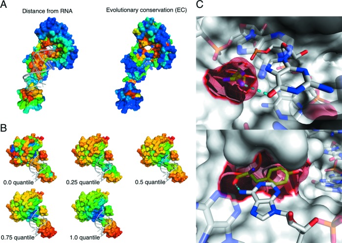
Novel features used in this work. (A) EC. A surface representation of the class-I A. fulgidus CCA-adding enzyme bound to a tRNA fragment (PDB ID: 3OVB). A distance map between protein and bound RNA with near (far) residues colored red (blue) is shown on the left. The EC value with high (low) colored red (blue) is shown on the right. (B) LN under a series of scales. LN values increase from blue to red. At each granularity level, warmer colors indicate convex residues, while cooler color represents concave residues. (C) Solvent ASA. A surface representation of RNase Cas6 (PDB ID: 4ILL) is shown. The protein makes both side-chain and backbone contacts with substrate RNA. Target residues (meshed) and nucleotides are represented by opaque sticks, connected by hydrogen bonds (dashed lines). The side chain of R268 protrudes and binds G15 (top). The backbone of Y168, which is mostly buried and forms part of a cleft, interacts with A5 (bottom). All figures of 3D structure representation in this work were generated by PyMOL Molecular Graphics System, Version 1.5, Schrödinger, LLC.

Describing structural features with normalized Laplacian coordinates

We next investigated the effect of adding structural information via LN coordinates, which are a description of the protein based on graph theory with a single parameter (σ) that controls the resolution or granularity of the model (see Materials and Methods). When taking norms of the Laplacian coordinates, information regarding the absolute target residue spatial position is lost. For this reason, a combination of the sequence-based control features and LN values calculated under any given σ value (global or local) failed to augment the AUC of the ROC curve significantly. Interestingly, however, when we built up a multidimensional LN vector at multiple σ levels, the discrimination power of the neural network was significantly enhanced. The reason for this is that missing positional information due to norm calculation was compensated for by the set of LN values, which contain geometric information. Simply speaking, buried residues have a smaller average LN value than exposed ones. For exposed residues under a given σ value, a large LN corresponds to a convex surface, while a small one reflects a concave surface.

We next investigated the relationship between protein–RNA distances and LN values, as well as the distribution of LN values on global and local scales (Supplementary Figure S5). On a global scale, as shown in Supplementary Figure S5A, the median value and the deviation of distances between surface residues and RNA increased with the normalized LN value (indicating a transition from concave to convex from left to right, respectively). However, as the LN value approached 1, the median distance decreased slightly. From the distribution patterns of LN values taken from RNA binding and non-binding residues, as well as all surface residues (Supplementary Figure S5B), we found that RNA-binding residues showed a statistically significant (P-value < 1e-15) shift toward smaller LN values when compared with non-binding residues or background residues, which means that RNA is more likely to interact with residues located on globally concave surfaces. Interestingly, the frequency of RNA-binding residues with a LN value close to 1 was also higher. These residues are located at extremely convex points. Next, we checked the distribution of local LN values for RNA-binding residues interacting with a globally concave surface (surface residues with global LN values smaller than 0.45 as shown in Supplementary Figure S5B). We can see from Supplementary Figure S5C that the distribution pattern shows two peaks; one exists at a relatively small local LN value, corresponding to concave surfaces, while the other exists at a moderately large value, indicating convex points. The frequency of contacts for flatter regions (i.e. around 0.5) was lower.

After manually checking many structures, a general rule could be summarized as follows: An RNA molecule is more likely to bind to globally concave surfaces of a protein, and to locally convex or concave sites within that milieu. On a local scale, however, convex (i.e. protruding) residues are more likely to mediate RNA contacts. In Figure 1B, LN values for the cys4-CRISPR RNA complex (PDB entry 4AL5) at different σ values are mapped onto the protein surface. ROC and PR curves based on non-ribosomal and the full dataset are given in Supplementary Figure S6. Here, the AUC increased 3.3 and 1.6% for the non-ribosomal and full sets, respectively, after combining the LN feature with the control sequence features.

Contributions from solvent ASA

We found that neither predicted absolute ASA nor relative ASA normalized by the ASA of the corresponding amino acid in an extended tripeptide (Ala-X-Ala) could noticeably improve classifier performance, in agreement with another study (16). This arises, in part, from the fact that RNA can make contact with an exposed amino acid side chain even when the backbone is buried or conversely with an exposed backbone with a buried side chain, as illustrated in Figure 1C. Thus, overall residue ASA is not necessarily the best predictor of RNA-binding propensity. In particular, in the case of non-specific interactions involving the protein backbone, overall residue ASA can be much smaller than that of the residue as a whole. Using our novel normalization procedure, however, which splits the ASA into three components (total, side chain and main chain), RNA-binding and non-binding residues could be distinguished, with an increase in the AUC of 1.9 and 1.3% for the non-ribosomal and full sets, respectively (Supplementary Figure S7). Here, a neighbor list of length 11 was used to include information about residues in a local surface patch.

Physicochemical prosperities of neighboring residues and predicted secondary structure

We found that both physicochemical features encoded from a neighboring residue list in an ascending distance order (Supplementary Figure S8), or predicted secondary structure for a sequential residue fragment (Supplementary Figure S9) could modestly increase the performance of the neural network. For the physicochemical feature, a neighbor list of length 21 was used. For the predicted secondary structure, a sliding window of size 5 was used.

Putting it all together

After combining the above-mentioned sequence (including the terms used in the control method) and structural features, we compared the performance of our model with that using only the sequence-based control method. The number of columns for each kind of feature and the size of fragment window used (either a sequential window or a spatial window) are summarized in Table 1. A performance summary of individual features and all features combined together can be found in Table 2. Finally for each coding fragment window, a 668-column feature vector was used. We found that our novel feature-coding scheme could significantly increase the prediction performance not only in terms of the AUC but also in terms of PR measurements for both datasets, as shown in Figure 2 (non-ribosomal and full ROC and PR curves for binary prediction) and Supplementary Figures S10 and S11 (di-nucleotide curves for non-ribosomal and full sets). Importantly, contributions from different features were approximately additive, resulting in an increase in the AUC of 6.8 and 4.1% for the non-ribosomal and full sets, respectively, which indicates a low redundancy between features. The new features that contributed the most information were the LN and the normalized ASA. When using the EC feature instead of the PSSM feature, the performance decreased only slightly (data not shown). This is a non-trivial result as the PSSM feature requires 20 columns for each residue while the EC feature requires just one. Therefore the novel features described here are both information-rich and relatively compact. From the PR plots, we can see that, when training with the non-ribosomal dataset, the highest precision approached only 0.7 when sensitivity was extremely low. In contrast, the sensitivity values estimated from the complete dataset under a precision rate of 0.7 approached 1 (P-value of t-test < 1e-12). In contrast, with the full dataset, which contains twice the number of RNA binding sites, precision approached 1.0 at low sensitivity. Therefore, the neural network could learn from ribosomal proteins in the full dataset and achieve a better prediction even on non-ribosomal complexes. This implies that, although ribosomal and non-ribosomal proteins may be different in their RNA binding modes, they apparently share common features as well. We only considered RNA-binding residues under a 3.5 Å distance cutoff within the same BU as ‘true’; consequently, non-binding residues made up 89.4% of our RB205 dataset. This ratio was ∼85% when using a 5 Å distance cutoff for RNA-binding residues. In the best performing model (average sensitivity and specificity 0.775, sensitivity 0.763 and specificity 0.787) on the RB205 dataset, non-binding residues were predicted to be 72.9%.

Table 1. Summary of feature columns and fragment sizes.

Feature Name	No. of columns	No. of residues per fragment window
21-bit Sparse Coding	21 per residue	11 sequential residues (a sliding window of size 5)
GAC	20 per fragment	whole protein sequence
PSSM	20 per residue	11 sequential residues
EC	1 per residue	11 sequential residues
LN	5 per residue	11 sequential residues
Normalized ASAs	3 per residue	11 spatial residues (a neighboring window of size 10)
Physicochemical (PC) property	10 per fragment	21 spatial residues (a neighboring window of size 20)
Predicted secondary structure	8 per residue	11 sequential residues

Since the GAC is calculated from a single protein sequence, for each coding fragment, a GAC vector will be appended. For the PC feature, for a coding fragment a list of 21 neighboring residues will return 10 values.

Table 2. Performance summary of individual features and all features combined together.

Feature name	Non-ribosomal dataset	Complete dataset
Sequence-based control (SBC)	0.728 +/−0.001	0.812 +/−0.001
SBC + EC	0.741 +/−0.001	0.8196 +/−0.0003
SBC + LN	0.761 +/−0.001	0.828 +/−0.001
SBC + Normalized ASAs	0.7468 +/−0.0004	0.8253 +/−0.0007
SBC + Physicochemical (PC) property	0.7424 +/−0.0007	0.820 +/−0.001
SBC + Predicted secondarystructure	0.7374 +/−0.0004	0.8185 +/−0.0008
All together	0.796 +/−0.001	0.8526 +/−0.0008

Performance is measured in terms of AUC (mean ± Std) evaluated from five repetitions of five-fold cross-validation. SBC method indicates the sequence features that adapted from the SRCPred method (12).

Figure 2.

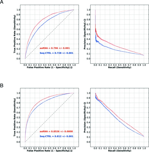
Performance of all features. (A) Non-ribosomal dataset. Blue curves indicate the performance of the control method (sequence features used in the SRCPred method (12)), and red curves show the performance when all features are used. (B) Full dataset. By varying the output cutoff of the classifier, the TP rate against the FP rate is plotted on the ROC curve for each cutoff value. Similarly, the precision rate against the TP rate is plotted on the PR curve for each cutoff value.

We next took a closer look at the reasons for FP and FN predictions. We found that FP could be evolutionarily conserved, exposed or charged, which could indicate a role in mediating protein–protein interactions rather than protein–RNA interactions. Though use of the LN feature suppressed such FP to a great extent, some residues localized at protein–protein interfaces that were chemically similar to RNA-binding residues were incorrectly positively predicted. With regard to the FN predictions, to a certain degree these were due to the ASA term. That is, relatively buried RNA-binding residues are harder to correctly identify as part of a binding site. Note that the relative importance among RNA-binding residues is also a factor. Some residues are crucial while others are more auxiliary. Residues that surround other residues in strong RNA contact are classified as RNA binding according to the distance criterion but might play a more important role in supporting the structure of the binding site than in mediating RNA contact directly. Our predictor overlooked some of these supporting residues and aaRNA is expected to perform better at identifying core binding residues than auxiliary residues. Finally, some exposed and protruding residues in RNA contact were predicted to be non-binding due their local environment; after averaging over neighboring residues the ASA of the protruding residue can be reduced.

Robustness to structural noise

Since the performance of structure-based classifiers could be over-estimated when input structures are in their RNA-bound conformations, we tested the robustness of our model by using structures built by homology modeling using template structures selected within various sequence identity thresholds. The distribution of templates under five sequence identity thresholds is shown in Supplementary Figure S12. The number of protein chains that was modeled under different identity thresholds and their averaged root-mean-square deviation from native structures are listed in Supplementary Table S3. Note that even when using templates from the top group, where sequence identity can be as high as 100%, predicted structures were not identical to the template because we carried out energy minimization on the models without RNA. Also, depending on the template, the number of predicted residues differed in general, especially when low sequence identity templates were used. Therefore, under different sequence identity cutoffs, we rebuilt the PDB dataset to include only residues that could be reproduced in the model. Performance evaluated on the homology models built using the five different sequence identity thresholds are listed in Figure 3. We can see that, even at a lowest sequence identity threshold (<30%), incorporating structural features was significantly better than using sequence features alone. Moreover, when high quality but non-identical templates were used (identity <100%), the AUC was nearly identical to that of the bound structure. These results imply that the aaRNA method is robust against typical levels of input noise.

Figure 3.

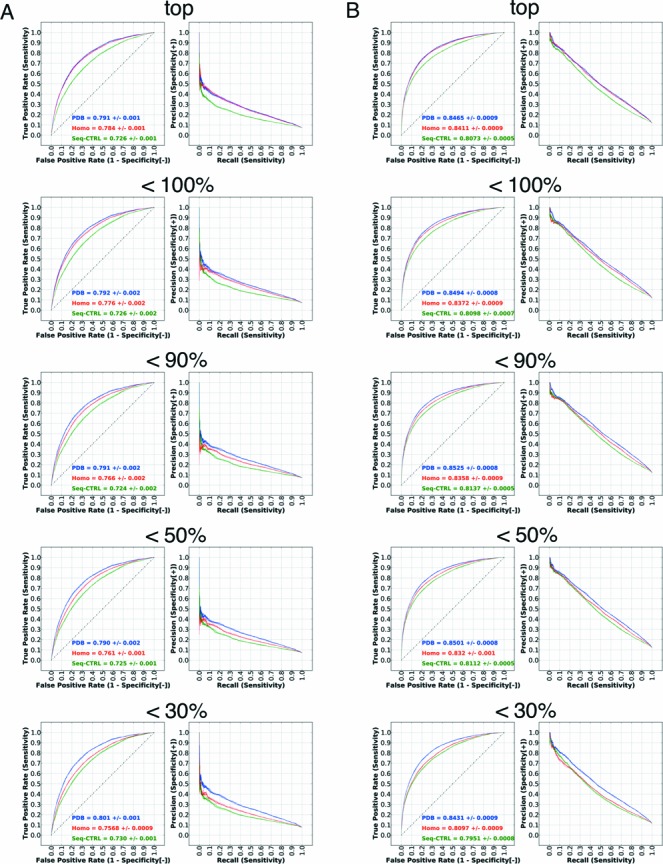
Performance evaluation using homology models. The left panel (A) shows the performance on the non-ribosomal set and the right panel (B) shows the performance on the full set. The figure shows the performance for the top, <100%, <90%, <50% and <30% homologs in subfigures. Since the number of residues generally decreases as the threshold is lowered, performance is only comparable within a given set. The performance using bound structures, homology models and sequence-based control are indicated by ‘PDB’, ‘Homo’ and ‘Seq-CTRL’.

Benchmark testing on RB106, RB144, RB198, RB44 and RB67

According to a recent study using a 5 Å cutoff to define RNA-binding (16), the AUC of different classifiers using PSSM features and their derivatives varied from 0.77 to 0.81. The best-performing method was the predictor RNABindR 2.0. In the aforementioned study, a balanced training dataset of positive and undersampled negative residues was prepared, while in our tests the datasets represented the actual distributions observed in the PDB, in which there are far more non RNA-binding residues. Nevertheless, when trained and tested on three standard benchmark datasets (RB106, RB144 and RB198) and evaluated in the same way (residue-based and protein-based evaluation on structure data), our additional features exhibited considerable improvement over sequence-based features alone, and exceed the previously reported AUC limit of 0.81 by 2–3%, as demonstrated in Figure 4. In Table 3 the results of these three benchmark tests are summarized. Performance differences were assessed both at the residue level (Benchmark [r]) and at the protein level (Benchmark [p]). The AUC distribution of the protein-chain based evaluation is shown in Supplementary Figure S13. In both residue-level and protein-level assessments the improvement in performance of aaRNA over the alternative methods was highly significant (P-values <10⁻⁵ and <10⁻¹⁰, respectively). To be complete, the number of RNA-binding and non-binding residues in the three benchmark datasets collected under a 3.5 or 5 Å distance cutoff are listed in the Supplementary Table S2. The performance of our model built from three benchmark datasets using a <3.5 Å cutoff as the RNA-binding definition can be found in Supplementary Figure S14. When a smaller cutoff was used, performances of models on three benchmarks all increased.

Figure 4.

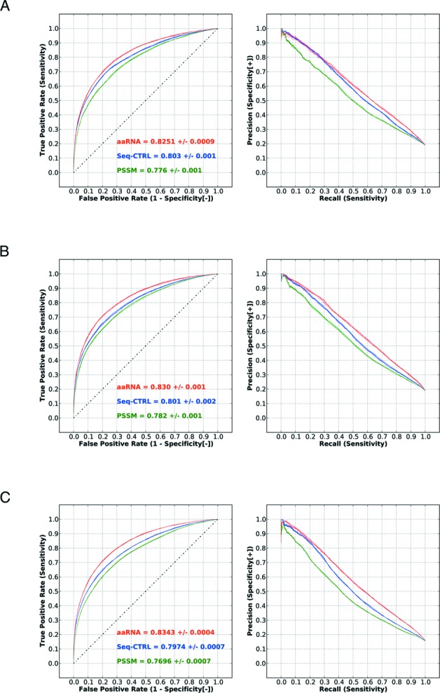
Performance of our feature-coding scheme on three benchmark datasets under a 5 Å distance cutoff for RNA-binding residues. The three benchmarks shown are RB106 (A), RB144 (B) and RB198 (C). The label ‘PSSM’ indicates the AUC achieved with PSSM features only. The label ‘Seq-CTRL’ indicates the result with the sequence-based control and the label ‘aaRNA’ for all of our proposed features.

Table 3. Summary of benchmark (RB106, RB144 and RB198) results in terms of AUC (mean ± Std).

Benchmark [r]	RNABindR 2.0	PSSM	Sequence-based control	aaRNA
RB106	0.81	0.776 ± 0.001 *	0.803 ± 0.001 *	0.8251 ± 0.0009
RB144	0.81	0.782 ± 0.001 *	0.801 ± 0.002 *	0.830 ± 0.001
RB198	0.80	0.7696 ± 0.0007 *	0.7974 ± 0.0007 *	0.8343 ± 0.0004
Benchmark [p]	RNABindR 2.0	PSSM	Sequence-based control	aaRNA
RB106	0.74	0.721 ± 0.119 **	0.735 ± 0.109 **	0.765 ± 0.116
RB144	0.74	0.723 ± 0.118 **	0.733 ± 0.111 **	0.778 ± 0.105
RB198	0.73	0.716 ± 0.114 **	0.738 ± 0.106 **	0.784 ± 0.103

The corresponding ROC plots and AUC distribution patterns are given in Figure 4 (residue-based evaluation) and Supplementary Figure S13 (protein-based evaluation), respectively. RNABindR 2.0 is the best-performing sequence-based method from various approaches evaluated in the work (16). Its reported performance is listed. Sequence-based control method represents three sequence features of the aaRNA, which are adapted from the work SRCPred (12). In Benchmark [r], AUCs were measured on a protein-residue basis, and reported AUCs are the average results of five repetitions of five-fold cross-validation. The average AUC of the aaRNA method is significantly greater than that of the PSSM or sequence-based control method using a t-test. In Benchmark [p], AUCs were individually calculated for each protein chain, and a paired Wilcoxon test was applied to check whether the distribution of the aaRNA AUC is shifted to the right relative to that of the PSSM and sequence-based control. The significance of differences between the alternative methods and aaRNA is indicated by * for P-values < 10^-5 and ** for P-values < 10^-10.

In prediction tests, the same RNA-binding residue distance cutoff of 3.5 Å was used. Prediction comparison between aaRNA and BindN+ methods based on merged and cleaned RNABindR 2.0 datasets is shown in Supplementary Figure S15. We can see that the aaRNA method outperformed the BindN+ method in terms of AUC. In addition, when applying our model to the RB44 dataset, which has no structures in common with our training dataset, our model achieved better performance than the sequence and structure-based methods tested in (16,30) in most cases. Using a residue-based evaluation, the AUC, MCC and F-score calculated from our predictions were 0.8445, 0.483 and 0.593 (see Table 4), respectively, in contrast to the author's Meta-predictor (30), which achieved an AUC of 0.835 and an MCC of 0.460. This Meta-predictor was built from three best-performing predictors out of seven sequence-based methods evaluated in (30), and performed better than any of its component methods. Using a protein-based evaluation, aaRNA achieved better performance than other sequence or structure-based predictors in terms of MCC except the DRNA method, the MCC of which is close to and slightly higher than the aaRNA method. We noticed that on a protein basis, the structure-based method DRNA was accurate when predicting proteins structurally similar to those in the training set. When query structures were uncharacterized by the predictor before (e.g. the RB67 benchmark), the prediction error was more substantial, as shown in Table 5. In spite of the fact that the mean MCC of the DRNA on the RB44 dataset is still high after making average over all protein chains, the prediction accuracy is limited when new protein structures are introduced. A detailed comparison of Accuracy, Specificity [+] (Precision), Sensitivity, F-measure, MCC and AUC (if available from the predictors) on the RB44 benchmark can be found in Table 4. A comparison of ROC and PR curves is given in Supplementary Figure S16A. Since the number of residues in the raw RB44 dataset and the homology model datasets are different, prediction results for the two methods are not directly comparable. However, as Supplementary Figure S16B shows, use of homology models does not impair aaRNA AUC significantly, suggesting that the performance reported here is robust against such small changes in the input data. When testing different predictors on the most up-to-date RB67 benchmark, aaRNA performed better than all other predictors either on a residue- or a protein-basis. Structural features introduced in aaRNA shed some light on the hallmarks of RNA-binding residues common to various RNA-binding proteins, which resulted in higher prediction power when exploring novel proteins. Results for the RB67 benchmark are listed in Table 5. The corresponding AUC and PR curves can be found in Supplementary Figure S17.

Table 4. Summary of the independent benchmark RB44 results in terms of MCC.

Evaluation	Method	Accuracy	Specificity [+] (Precision)	Sensitivity (Recall)	F-measure	MCC	AUC
	aaRNA	0.823	0.551	0.643	0.593	0.483	0.845
	BindN+	0.835	0.614	0.468	0.531	0.439	0.819
Residue-	RNAbindR 2.0	0.805	0.514	0.532	0.523	0.401	0.801
based	Seq-CTRL	0.804	0.510	0.600	0.552	0.430	0.807
	KYG	0.771	0.449	0.638	0.527	0.392	0.808
	DRNA	0.788	0.480	0.660	0.556	0.430	N/A
	OPRA	0.746	0.403	0.551	0.465	0.311	N/A
	aaRNA	0.793	0.477	0.625	0.525	0.395	0.819
	BindN+	0.755	0.429	0.699	0.520	0.380	0.791 *
Protein-	RNAbindR 2.0	0.737	0.415	0.593	0.474	0.326	0.761 **
based	Seq-CTRL	0.763	0.459	0.547	0.473	0.343	0.782 ***
	KYG	0.727	0.397	0.672	0.486	0.334	0.775 ****
	DRNA	0.776	0.482	0.618	0.521	0.400	N/A
	OPRA	0.727	0.346	0.467	0.362	0.211	N/A

The same RNA-binding residue distance cutoff of 3.5 Å was used. Two evaluation methods (residue-based and protein-based) are used to estimate the performance of different predictors. Because the output of DRNA and OPRA methods provides no score describing residues’ RNA-binding propensities, an ROC analysis cannot be performed to estimate their AUCs. Except the DRNA method evaluated on a protein basis, which got a slightly higher MCC, aaRNA achieved better MCCs and AUCs than other sequence or structure-based methods, both in residue-based and protein-based performance evaluation. Paired Wilcoxon tests on protein-averaged AUCs of aaRNA and other methods indicated significant differences (P* < 3e-4, P** < 8e-7, P*** < 5e-8 and P**** < 2e-4).

Table 5. Summary of the independent benchmark RB67 results in terms of MCC.

Evaluation	Method	Accuracy	Specificity [+] (Precision)	Sensitivity (Recall)	F-measure	MCC	AUC
	aaRNA	0.882	0.437	0.494	0.464	0.399	0.842
	BindN+	0.862	0.372	0.491	0.423	0.351	0.814
Residue-	RNAbindR 2.0	0.867	0.376	0.438	0.404	0.331	0.798
based	Seq-CTRL	0.886	0.443	0.401	0.421	0.358	0.811
	KYG	0.804	0.274	0.542	0.364	0.284	0.780
	DRNA	0.842	0.298	0.392	0.339	0.254	N/A
	OPRA	0.843	0.301	0.403	0.345	0.261	N/A
	aaRNA	0.844	0.428	0.449	0.398	0.323	0.814
	BindN+	0.828	0.377	0.463	0.397	0.301	0.780 *
Protein-	RNAbindR 2.0	0.750	0.296	0.616	0.372	0.272	0.764 **
based	Seq-CTRL	0.797	0.355	0.488	0.372	0.286	0.787 ***
	KYG	0.769	0.298	0.505	0.349	0.240	0.716 ****
	DRNA	0.795	0.319	0.397	0.331	0.229	N/A
	OPRA	0.797	0.242	0.259	0.203	0.116	N/A

Different predictors were compared in the same way as the RB44 benchmark. When tested on this up-to-date benchmark, the aaRNA got a superior performance than all others. Paired Wilcoxon tests on protein-averaged AUCs of aaRNA and other methods indicated significant differences (P* < 2e-4, P** < 2e-5, P*** < 7e-5 and P**** < 4e-9).

In addition to the benchmark tests presented above, we provide an illustrative example in Figure 5, the Csy4-crRNA complex. In general, sequence-based predictors were more likely to predict charged, polar or aromatic residues on the surface as positive binding sites regardless of their local structural environment. In contrast, due to spatial features introduced here, aaRNA gave more priority to such residues when localized in characteristic RNA binding sites, as learned from the training set. Hence, the aaRNA method could effectively decrease the number of FP predictions, as compared to Figure 5C, E, and F. Importantly, these structural features could facilitate identification of RNA binding sites that are invisible from the point of view of the linear amino acid sequence. As a result, more residues in actual RNA contact could be predicted by aaRNA, and the resulting binding patch appeared more native-like, as illustrated in Figure 5B and C.

Figure 5.

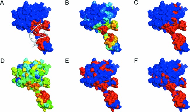
Comparison of prediction results of aaRNA, BindN+ and SRCPred. The figure shows the Csy4-crRNA complex (PDB entry 4AL5). (A) actual contact pattern of the complex. Red colored residues are in RNA contact under a 3.5 Å cutoff. (B) mapping of aaRNA binary binding propensities onto residues, with high (low) colored red (blue). (C) residues in red are positively predicted by the aaRNA under a stringency of 85% expected specificity. (D–E) show the raw and the threshold-calibrated (85% expected specificity), respectively, for BindN+ colored in the same way. (F) prediction results for SRCPred for any di-nucleotide under a 0.05 expected precision.

aaRNA server

The aaRNA server was built by using the model trained from the complete dataset (RB205). The aaRNA server accepts protein sequences or structures in FASTA and PDB formats, respectively. Structures can be input as PDB identifiers or files in PDB format. When only sequence information is provided, a homology model will be built in advance of the prediction. When a structure includes multiple chains that function together as a complex, the complex can be treated as a single entity or split into individual chains and the features will be computed accordingly. The output includes binary (binding/non-binding) and di-nucleotide propensities as a list of scores (between 0 and 1) indexed by the residue number of the target protein. A plot is also displayed showing the binary and di-nucleotide binding propensities. Users can refer to the di-nucleotide specific binding probabilities in addition to the binary scores when target RNA is enriched with a specific di-nucleotide composition or certain types of di-nucleotides are of interest. To facilitate analysis, surface maps of EC, LN under local and global scales, and binary binding propensities are displayed side by side in JSmol Applets on the result page. A high-quality surface map can be locally reproduced with Pymol after downloading a tar-compressed file for this purpose. Depending on the query protein, the time used for prediction can vary significantly. Once a job is finished, users will be notified by email with a link containing the result page.

DISCUSSION

In this study, we have looked at protein–RNA interactions from the point of view of the protein and attempted to predict where and in what way an RNA molecule would bind. If we consider the most general case, as represented by the ‘full’ dataset, Figure 2B indicates an AUC-based accuracy of 85%. This value can be interpreted as the probability that a randomly chosen ‘true’ RNA-binding residue will be ranked above a randomly chosen ‘false’ RNA-binding residue. If we examine the corresponding PR curve, we can see that there is a roughly linear tradeoff between precision (defined as the faction of predicted residues that are true RNA binders) and recall (the fraction of true RNA binders predicted). This, in turn, indicates that we can associate a residue-level confidence with our predictions, a result that is useful for downstream analysis. In terms of such analysis, we currently envision two concrete outcomes from this work, one global and one local.

A global approach is to use aaRNA to identify novel RNA-binding proteins on a genomic scale. This would potentially be beneficial if used in tandem with other high-throughput analyses such as microarray or RNAseq-based gene expression data. Since many such datasets have already been made public for cell lines of interest to specific research domains, such as immunology (https://www.immgen.org) or cancer (http://lifesciencedb.jp/cged/), data mining for RNA-binding proteins could facilitate further discrimination between transcriptional and post-transcriptional regulation of gene expression. Currently, aaRNA has only been applied to bona fide RNA-binding proteins, and no attempt has been made to distinguish binders from non-binders. However, such a binary classification would appear to be a natural extension that is not biased toward obvious RNA binding motifs.

A more local extension of the current work would be to utilize predicted RNA binding propensities in protein–RNA docking simulations. Current docking methods are not optimized for protein–RNA interactions and there is no standard statistics-based potential for such studies. Obvious contributions to the binding energy, such as electrostatics, surface burial, etc., can be computed, but there is not currently an established framework for combining them into an overall score. The importance of charged, polar and aromatic protein residues to RNA-binding has been reported previously (36,37); however, considering the fact that the number of possible Van der Waals contacts between protein and target RNA (∼92% of total interactions) exceeds by far the number of hydrogen bond contacts, an equally important factor to protein–RNA interaction could be shape complementarity at the binding interface. Since RNA is a highly flexible molecule, it makes practical sense to map RNA-binding propensities onto relatively rigid protein molecular surfaces. RNA-folding methods in combination with flexible docking could then be used to generate models for downstream experimental validation. This type of approach would be particularly attractive for transient protein–RNA interactions, which are likely to occur in situations such as regulation of mRNA decay, host-pathogen interactions and processing of noncoding RNAs. Along these lines, one way of improving prediction accuracy will be to take RNA folding into consideration. While this will by no means be easy, aaRNA provides a foundation for such future endeavors.

SUPPLEMENTARY DATA

Supplementary Data are available at NAR Online.

REFERENCES

- 1.Glisovic T., Bachorik J.L., Yong J., Dreyfuss G. RNA-binding proteins and post-transcriptional gene regulation. FEBS Lett. 2008;582:1977–1986. doi: 10.1016/j.febslet.2008.03.004. [DOI] [PMC free article] [PubMed] [Google Scholar]
- 2.Hogan D.J., Riordan D.P., Gerber A.P., Herschlag D., Brown P.O. Diverse RNA-binding proteins interact with functionally related sets of RNAs, suggesting an extensive regulatory system. PLoS Biol. 2008;6:e255. doi: 10.1371/journal.pbio.0060255. [DOI] [PMC free article] [PubMed] [Google Scholar]
- 3.Licatalosi D.D., Darnell R.B. RNA processing and its regulation: global insights into biological networks. Nat. Rev. Genet. 2010;11:75–87. doi: 10.1038/nrg2673. [DOI] [PMC free article] [PubMed] [Google Scholar]
- 4.Ramakrishnan V., White S.W. Ribosomal protein structures: insights into the architecture, machinery and evolution of the ribosome. Trends Biochem. Sci. 1998;23:208–212. doi: 10.1016/s0968-0004(98)01214-6. [DOI] [PubMed] [Google Scholar]
- 5.Patel A.A., Steitz J.A. Splicing double: insights from the second spliceosome. Nat. Rev. Mol. Cell Biol. 2003;4:960–970. doi: 10.1038/nrm1259. [DOI] [PubMed] [Google Scholar]
- 6.Matsushita K., Takeuchi O., Standley D.M., Kumagai Y., Kawagoe T., Miyake T., Satoh T., Kato H., Tsujimura T., Nakamura H., et al. Zc3h12a is an RNase essential for controlling immune responses by regulating mRNA decay. Nature. 2009;458:1185–1190. doi: 10.1038/nature07924. [DOI] [PubMed] [Google Scholar]
- 7.Wu J., Bera A.K., Kuhn R.J., Smith J.L. Structure of the Flavivirus helicase: implications for catalytic activity, protein interactions, and proteolytic processing. J. Virol. 2005;79:10268–10277. doi: 10.1128/JVI.79.16.10268-10277.2005. [DOI] [PMC free article] [PubMed] [Google Scholar]
- 8.Felden B. RNA structure: experimental analysis. Curr. Opin. Microbiol. 2007;10:286–291. doi: 10.1016/j.mib.2007.05.001. [DOI] [PubMed] [Google Scholar]
- 9.Murakami Y., Spriggs R.V., Nakamura H., Jones S. PiRaNhA: a server for the computational prediction of RNA-binding residues in protein sequences. Nucleic Acids Res. 2010;38:W412–W416. doi: 10.1093/nar/gkq474. [DOI] [PMC free article] [PubMed] [Google Scholar]
- 10.Wang L., Huang C., Yang M.Q., Yang J.Y. BindN+ for accurate prediction of DNA and RNA-binding residues from protein sequence features. BMC Syst. Biol. 2010;4(Suppl. 1):S3. doi: 10.1186/1752-0509-4-S1-S3. [DOI] [PMC free article] [PubMed] [Google Scholar]
- 11.Ma X., Guo J., Wu J., Liu H., Yu J., Xie J., Sun X. Prediction of RNA-binding residues in proteins from primary sequence using an enriched random forest model with a novel hybrid feature. Proteins. 2011;79:1230–1239. doi: 10.1002/prot.22958. [DOI] [PubMed] [Google Scholar]
- 12.Fernandez M., Kumagai Y., Standley D.M., Sarai A., Mizuguchi K., Ahmad S. Prediction of dinucleotide-specific RNA-binding sites in proteins. BMC Bioinformatics. 2011;12(Suppl. 13):S5. doi: 10.1186/1471-2105-12-S13-S5. [DOI] [PMC free article] [PubMed] [Google Scholar]
- 13.Kim O.T., Yura K., Go N. Amino acid residue doublet propensity in the protein-RNA interface and its application to RNA interface prediction. Nucleic Acids Res. 2006;34:6450–6460. doi: 10.1093/nar/gkl819. [DOI] [PMC free article] [PubMed] [Google Scholar]
- 14.Zhao H., Yang Y., Zhou Y. Structure-based prediction of RNA-binding domains and RNA-binding sites and application to structural genomics targets. Nucleic Acids Res. 2011;39:3017–3025. doi: 10.1093/nar/gkq1266. [DOI] [PMC free article] [PubMed] [Google Scholar]
- 15.Perez-Cano L., Solernou A., Pons C., Fernandez-Recio J. Structural prediction of protein-RNA interaction by computational docking with propensity-based statistical potentials. Pac. Symp. Biocomput. 2010;15:293–301. doi: 10.1142/9789814295291_0031. [DOI] [PubMed] [Google Scholar]
- 16.Walia R.R., Caragea C., Lewis B.A., Towfic F., Terribilini M., El-Manzalawy Y., Dobbs D., Honavar V. Protein-RNA interface residue prediction using machine learning: an assessment of the state of the art. BMC Bioinformatics. 2012;13:89. doi: 10.1186/1471-2105-13-89. [DOI] [PMC free article] [PubMed] [Google Scholar]
- 17.Hopf T.A., Colwell L.J., Sheridan R., Rost B., Sander C., Marks D.S. Three-dimensional structures of membrane proteins from genomic sequencing. Cell. 2012;149:1607–1621. doi: 10.1016/j.cell.2012.04.012. [DOI] [PMC free article] [PubMed] [Google Scholar]
- 18.Bonnel N., Marteau P.F. LNA: fast protein structural comparison using a Laplacian characterization of tertiary structure. IEEE/ACM Trans. Comput. Biol. Bioinform. 2012;9:1451–1458. doi: 10.1109/TCBB.2012.64. [DOI] [PubMed] [Google Scholar]
- 19.Berman H.M., Coimbatore Narayanan B., Di Costanzo L., Dutta S., Ghosh S., Hudson B.P., Lawson C.L., Peisach E., Prlic A., Rose P.W., et al. Trendspotting in the Protein Data Bank. FEBS Lett. 2013;587:1036–1045. doi: 10.1016/j.febslet.2012.12.029. [DOI] [PMC free article] [PubMed] [Google Scholar]
- 20.McDonald I.K., Thornton J.M. Satisfying hydrogen bonding potential in proteins. J. Mol. Biol. 1994;238:777–793. doi: 10.1006/jmbi.1994.1334. [DOI] [PubMed] [Google Scholar]
- 21.Remmert M., Biegert A., Hauser A., Soding J. HHblits: lightning-fast iterative protein sequence searching by HMM-HMM alignment. Nature methods. 2012;9:173–175. doi: 10.1038/nmeth.1818. [DOI] [PubMed] [Google Scholar]
- 22.Hamming R.W. Error detecting and error correcting codes. At&T Tech. J. 1950;29:147–160. [Google Scholar]
- 23.Charif D., Lobry J. In: Structural Approaches to Sequence Evolution. Bastolla U., Porto M., Roman H.E., Vendruscolo M., editors. Berlin Heidelberg: Springer; 2007. pp. 207–232. [Google Scholar]
- 24.Kabsch W., Sander C. Dictionary of protein secondary structure: pattern recognition of hydrogen-bonded and geometrical features. Biopolymers. 1983;22:2577–2637. doi: 10.1002/bip.360221211. [DOI] [PubMed] [Google Scholar]
- 25.Lis M.K.T., Sarmiento J.J., Kuroda D., Dinh H.V., Kinjo A.R., Amada K., Devadas S., Nakamura H., Standley D.M. Bridging the gap between single-template and fragment based protein structure modeling using Spanner. Immun. Rese. 2011;7:1–8. [Google Scholar]
- 26.Soding J., Biegert A., Lupas A.N. The HHpred interactive server for protein homology detection and structure prediction. Nucleic Acids Res. 2005;33:W244–W248. doi: 10.1093/nar/gki408. [DOI] [PMC free article] [PubMed] [Google Scholar]
- 27.Terribilini M., Lee J.H., Yan C., Jernigan R.L., Honavar V., Dobbs D. Prediction of RNA binding sites in proteins from amino acid sequence. Rna. 2006;12:1450–1462. doi: 10.1261/rna.2197306. [DOI] [PMC free article] [PubMed] [Google Scholar]
- 28.Terribilini M., Sander J.D., Lee J.H., Zaback P., Jernigan R.L., Honavar V., Dobbs D. RNABindR: a server for analyzing and predicting RNA-binding sites in proteins. Nucleic Acids Res. 2007;35:W578–W584. doi: 10.1093/nar/gkm294. [DOI] [PMC free article] [PubMed] [Google Scholar]
- 29.Lewis B.A., Walia R.R., Terribilini M., Ferguson J., Zheng C., Honavar V., Dobbs D. PRIDB: a protein-RNA interface database. Nucleic Acids Res. 2011;39:D277–D282. doi: 10.1093/nar/gkq1108. [DOI] [PMC free article] [PubMed] [Google Scholar]
- 30.Puton T., Kozlowski L., Tuszynska I., Rother K., Bujnicki J.M. Computational methods for prediction of protein-RNA interactions. J. Struct. Biol. 2012;179:261–268. doi: 10.1016/j.jsb.2011.10.001. [DOI] [PubMed] [Google Scholar]
- 31.Kumar M., Gromiha M.M., Raghava G.P. Prediction of RNA binding sites in a protein using SVM and PSSM profile. Proteins. 2008;71:189–194. doi: 10.1002/prot.21677. [DOI] [PubMed] [Google Scholar]
- 32.Jones S., Daley D.T., Luscombe N.M., Berman H.M., Thornton J.M. Protein-RNA interactions: a structural analysis. Nucleic Acids Res. 2001;29:943–954. doi: 10.1093/nar/29.4.943. [DOI] [PMC free article] [PubMed] [Google Scholar]
- 33.Gupta A., Gribskov M. The role of RNA sequence and structure in RNA–protein interactions. J. Mol. Biol. 2011;409:574–587. doi: 10.1016/j.jmb.2011.04.007. [DOI] [PubMed] [Google Scholar]
- 34.Kondo J., Westhof E. Base pairs and pseudo pairs observed in RNA-ligand complexes. J. Mol. Recognit. 2010;23:241–252. doi: 10.1002/jmr.978. [DOI] [PubMed] [Google Scholar]
- 35.Kondo J., Westhof E. Classification of pseudo pairs between nucleotide bases and amino acids by analysis of nucleotide-protein complexes. Nucleic Acids Res. 2011;39:8628–8637. doi: 10.1093/nar/gkr452. [DOI] [PMC free article] [PubMed] [Google Scholar]
- 36.Treger M., Westhof E. Statistical analysis of atomic contacts at RNA-protein interfaces. J. Mol. Recognit. 2001;14:199–214. doi: 10.1002/jmr.534. [DOI] [PubMed] [Google Scholar]
- 37.Ellis J.J., Broom M., Jones S. Protein-RNA interactions: structural analysis and functional classes. Proteins. 2007;66:903–911. doi: 10.1002/prot.21211. [DOI] [PubMed] [Google Scholar]
Associated Data
This section collects any data citations, data availability statements, or supplementary materials included in this article.