A Tiered Framework for Risk-Relevant Characterization and Ranking of Chemical Exposures: Applications to the National Children’s Study (NCS)

Abstract

A challenge for large-scale environmental health investigations such as the National Children’s Study (NCS), is characterizing exposures to multiple, co-occurring chemical agents with varying spatiotemporal concentrations and consequences modulated by biochemical, physiological, behavioral, socioeconomic, and environmental factors. Such investigations can benefit from systematic retrieval, analysis, and integration of diverse extant information on both contaminant patterns and exposure-relevant factors. This requires development, evaluation, and deployment of informatics methods that support flexible access and analysis of multiattribute data across multiple spatiotemporal scales. A new “Tiered Exposure Ranking” (TiER) framework, developed to support various aspects of risk-relevant exposure characterization, is described here, with examples demonstrating its application to the NCS. TiER utilizes advances in informatics computational methods, extant database content and availability, and integrative environmental/exposure/biological modeling to support both “discovery-driven” and “hypothesis-driven” analyses. “Tier 1” applications focus on “exposomic” pattern recognition for extracting information from multidimensional data sets, whereas second and higher tier applications utilize mechanistic models to develop risk-relevant exposure metrics for populations and individuals. In this article, “tier 1” applications of TiER explore identification of potentially causative associations among risk factors, for prioritizing further studies, by considering publicly available demographic/socioeconomic, behavioral, and environmental data in relation to two health endpoints (preterm birth and low birth weight). A “tier 2” application develops estimates of pollutant mixture inhalation exposure indices for NCS counties, formulated to support risk characterization for these endpoints. Applications of TiER demonstrate the feasibility of developing risk-relevant exposure characterizations for pollutants using extant environmental and demographic/socioeconomic data.

1. INTRODUCTION

One of the major challenges facing large-scale environmental health investigations, such as the National Children’s Study (NCS), is adequate characterization of risk-relevant exposures to chemical contaminants. In the case of the NCS, this characterization is required both for mothers, before and during pregnancy, and for children. Further-more, such characterization is complicated by the fact that chemical exposures always occur in relation to specific activities and diverse microenvironments, and for complex mixtures composed of numerous agents rather than for individual species. Finally, these exposures always occur in the context of multiple dose- and risk-modifying genetic, physiological, biochemical, socioeconomic, and behavioral factors that may enhance or mitigate the effects of contaminants in a dynamic fashion across the intervals of exposure. Characterization of environmental exposures requires the systematic retrieval, analysis, and integration of diverse types of information from a wide variety of sources. A novel, flexible, “multitier” framework designed to accomplish these objectives by employing extant data available at the federal, regional, state and local levels, is presented here. This tiered exposure ranking (TiER) framework allows sequential and complementary implementation of both discovery-driven exploratory data analysis methods (also called “agnostic,” “hypothesis-free,” and “exposomic” methods^(1–4)) and hypothesis-driven approaches. The discovery-driven approaches constitute “tier 1” of this framework and employ high-throughput computational tools, similar to those used in bioinformatics (genomics, transcriptomics, proteomics, etc.) to conduct multivariate exploratory analyses of large data sets for identification of plausible patterns and associations. The outcomes of the exploratory analyses, combined with available mechanistic knowledge relevant to the particular phenomena that are studied, can then be used to formulate focused hypotheses regarding these phenomena.

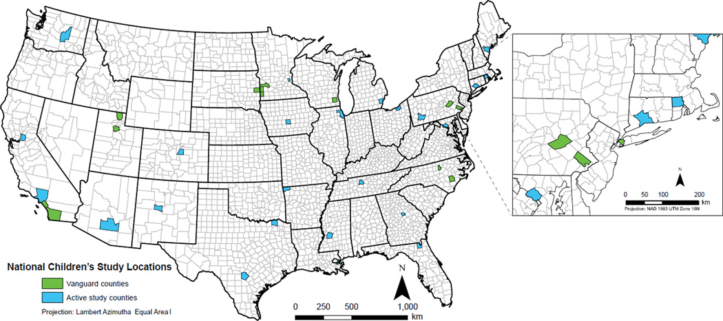
Higher-tier analyses of exposures within the TiER framework can be implemented in various ways: tier 2 characterization involves the use of extant data (as discussed below) in conjunction with simplified mechanistic modeling and allows rankings of risk-relevant exposures associated with particular “locations” (at county, census unit, study segment, or even individual residence levels). This is accomplished through development of distributional estimates of exposure for various relevant population subsets (or individuals) “assigned” to each particular location: distributions of risk-relevant exposures are calculated for multiple co-occurring agents associated with a common “adverse outcome pathway” (AOP) or “biological mode of action” (BMOA) for each exposure route (inhalation, ingestion, and dermal absorption). Due to the complexity of most exposures to mixtures, tier 2 calculations offer options to summarize and “condense” the information contained in the exposure distributions by calculating various exposure indices (EIs). These EIs provide screening rankings of risk-relevant cumulative and aggregate exposures and intakes associated with selected locations or subpopulations through a set of numerical values, or value ranges. The formulations of the EIs follow concepts and approaches similar to those used in previous studies of health risks from contaminant mixtures^(5–10) and can be customized to support or complement the testing of alternative environmental and biological hypotheses. As stated above, exposure agents incorporated in the formulation of particular EIs are selected on the basis of risk-relevant hypotheses involving common mechanisms and/or endpoints. When such hypotheses are not available, alternatively, exposure agents associated with a particular class of pollution sources, e.g., contaminants related to traffic emissions, can be selected to formulate an appropriate EI for exploratory analysis. This new framework addresses the need for an approach that can “mine,” analyze, and condense information from the vast amount of disparate extant data collected by federal, state, and local agencies.^(11,12) Added value to the extant data is provided by the fact that their databases are routinely updated and adhere to a variety of quality assurance practices.⁽¹¹⁾ This ensures a stable, consistent, and cost-effective source of “renewable” exposure-relevant information. In the case of the NCS, its multidisciplinary nature and complexity require generation of accessible and easily expandable and updatable sets of quality information that will support testing of a wide spectrum of hypotheses. The TiER framework has been employed with extant data to rank risk-relevant exposures associated with selected health endpoints for each county in the NCS (Fig. 1). Furthermore, in addition to the current “national-level” NCS results presented here, a tier 2 application of this framework was tested in a separate study for the Queens County Vanguard Center segments.⁽¹³⁾

Fig. 1.

Maps showing active National Children’s Study (NCS) locations.

2. APPROACH AND METHODS

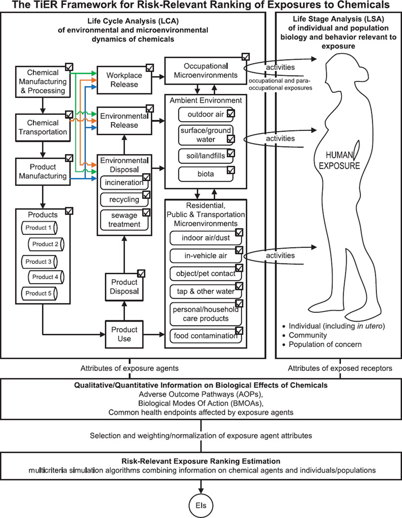
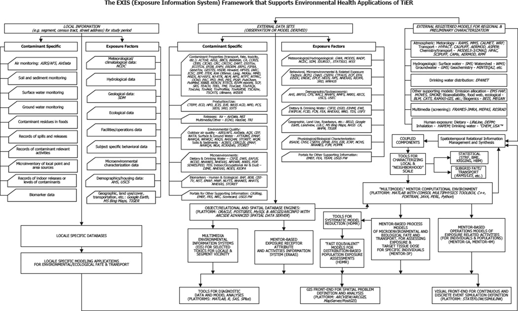
The TiER framework, schematically summarized in Fig. 2, employs computational components of the modular modeling systems Prioritization and Ranking of Toxic Exposures with GIS Extension (PRoTEGE)^(14,15) and Modeling Environment for Total Risk studies (MENTOR).^(16–20) Although MENTOR is a comprehensive simulation platform that has been evolving over the past 15 years, PRoTEGE is a new system that utilizes simplified versions of MENTOR components to provide screening-level analyses. State-of-the-art comprehensive uncertainty/variability and sensitivity analysis methods^(21–24) have been incorporated in both systems. Furthermore, a national-level multi-scale and multiattribute exposure information system (EXIS)^(11,25) has been constructed employing GIS and relational database platforms, and regularly updated over the past 15 years, to support applications of MENTOR; EXIS can also provide data sets usable by other modeling systems. A customized implementation of EXIS is used here to support characterization and ranking of exposures within the TiER framework (Fig. 3). More than 300 environmental and demographic data sets are currently incorporated in EXIS; the Electronic Appendix provides references and web links to a representative subset of the data utilized in the tier 1 and tier 2 analyses presented in Section 3.

Fig. 2.

Schematic representation of the tiered exposure ranking (TiER) framework for risk-relevant ranking of exposures to chemicals, incorporating (a) life cycle analysis (LCA) of environmental and microenvironmental dynamics of chemicals; (b) life stage analysis (LSA) of individual and population biology and behavior relevant to exposure; (c) qualitative/quantitative information on biological effects of chemicals for the selection and weighting/normalization of exposure agent attributes; and (d) multicriteria simulation algorithms combining information on chemical agents and individuals/populations for EI calculation.

Fig. 3.

A national-level multiscale exposure information system (EXIS) framework was constructed and is updated continually (over the past 15 years) to support applications of the MENTOR system; an implementation of this framework is used to support characterization and ranking of exposures within the TiER framework. (Table I lists the acronyms of databases and models appearing in this chart.)

For tier 1 analyses, PRoTEGE links with ebTrack,⁽²⁶⁾ a component of MENTOR that expands upon USFDA’s ArrayTrack⁽²⁷⁾ by incorporating tools for the multivariate analysis of environmental and demographic variables in addition to the analysis of “bionomic” (i.e., genomic, proteomic, metabalomic, etc.) data. An extensive set of exploratory data analysis routines implemented in Mat-lab and R complements these two systems.

Tier 1 exposure analyses via PRoTEGE and ebTrack consider a variety of attributes and metrics relevant to population exposures. The metrics can be based on data on contaminant releases and concentrations in relevant media for a location of concern, combined with information on plausible exposure and AOPs. The combined application of PRoTEGE and ebTrack on relevant environmental, demographic, behavioral, and biological data sets allows the exploratory identification of patterns and associations that can “sharpen” the focus of data collection efforts for the NCS and other environmental health studies.

In the following, the focus is limited to tier 2 characterization. Key outcomes of tier 2 characterization, as mentioned earlier, are EIs that attempt to capture available risk-relevant information for exposure ranking in a “minimal set” of numerical values. The following general equation is used to develop an exposure index (EI) for risks associated with a specific BMOA (or health endpoint) of interest, j:

$${\overrightarrow{E}}_j=\sum _k{g}_{j,k}(\overrightarrow{C_{\text{amb},j,k}}(s,t),{\overrightarrow{\psi }}_j(s,t),{\overrightarrow{\Phi }}_j(s,t),{\overrightarrow{\Omega }}_j(s)).$$

Each element of ${\overrightarrow{E}}_j$ is denoted by E_ij, where subscript i refers in general to a “location” (such as a county, a “segment” consisting of selected census tracts, or an actual “point” address) or the subpopulations/individuals associated with that location.

The variables appearing in the above equation are:

• Concentration fields $\overrightarrow{C_{\text{amb},j,k}}$ are measured or estimated spatiotemporal fields of co-occurring contaminant concentrations in various microenvironments (e.g., ambient air, indoor air, drinking water, residential water, food, dust, soil, etc.). For example, inhalation exposures, a focus of the initial TiER application, are calculated via a combination of the following methods: (i) spatiotemporal interpolation of ambient air quality monitoring data, (ii) prognostic air quality modeling, and (iii) Bayesian fusion of model outputs and monitor data. Subsequently, these terms are corrected for local neighborhood scale effects.⁽²⁸⁾ For cases of multi-route exposures to multimedia pollutants (e.g., pesticides and metals), additional characterization is required: the concentration fields in these cases must be developed for multiple media and pathways (food, drinking water, surface dust, and ambient air) using predictive models, as well as estimates from statistical models and analyses of available data.

• Microenvironmental attribute fields ${\overrightarrow{\Psi }}_j(s,t)$ are computed from study-specific data and supporting databases on population demographics, land use, topography, housing types and ages, etc.

• Exposure-activity pattern fields ${\overrightarrow{\Phi }}_j(s,t)$ are calculated (depending on the “tier”) from data relevant to the populations of concern retrieved from current extant databases such as CHAD⁽²⁹⁾ or from study-specific data and/or aggregation of representative time-activity diary information, commuting patterns, patterns of usage of consumer products, etc.

• Biological factors ${\overrightarrow{\Omega }}_j(s)$ are estimated from study-specific or representative population distributions of physiological and biochemical properties, with explicit consideration of pregnant women and their children. They include factors such as age and gender-specific distributions of inhalation and water intake rates, etc.

• Variables s and t denote the location and time vectors.

• A generalized weighting function g_{j, k} is typically contaminant-specific and can reflect the hypothesized relevance of the contaminant to the BMOA considered.

Note: Individual elements of each vector above themselves may represent either a continuous or discrete set of factors (concentration fields, housing characteristic attributes, etc.).

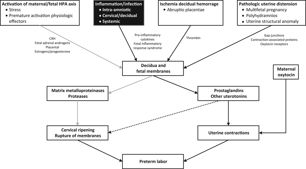
Formulation of a specific EI may consider information on the plausible health endpoint and consequently on the (hypothesized) relevant contaminants and exposure pathways. The pollutants and exposure pathways considered in defining an endpoint-specific EI can be selected based upon (i) literature reviews of proposed hypotheses regarding the particular health endpoint, (ii) literature reviews of related (epidemiological and clinical) studies, and (iii) exploratory multivariate analyses involving available data on the health outcome and exposure factors and contaminant levels. Since the scope of EIs is to provide a “screening” type of risk-relevant exposure ranking, the associated health outcome is selected (based on plausible hypotheses from the scientific literature) in relation to general BMOAs that are potentially relevant to the environmental agents of concern. The weighting functions in Equation (1) are thus developed by considering available reference concentrations (RfCs) or doses associated with these BMOAs. In the examples presented in Section 3 as applications of the TiER framework, inflammation is hypothesized as a plausible BMOA (Fig. 4) associated with the preterm birth (PB) and low birth weight (LBW) health endpoints. This hypothesis was used to select contaminants for tier 2 analysis (i.e., for the EI formulation and calculation).

Fig. 4.

Common biological pathways associated with preterm birth (chart adapted from Behrman and Butler⁽³³⁾); the demonstration study presented here uses inflammation as a plausible biological mode of action to select airborne agents for the formulation of an inhalation exposure index relating to preterm birth.

The models and data sets (see Fig. 3) available for estimating EIs within the TiER framework are peer-reviewed formulations for which standardized procedures and quality criteria exist for developing appropriate inputs. In cases where simplifying assumptions are made for the “original” peer-reviewed model so as to allow application in a “screening” or “range finding” mode, these assumptions and the associated uncertainty-related implications are explicitly documented. Special consideration is given to assessing appropriate spatial and temporal resolution limits that are reasonably allowed by extant data: for example, available national-level databases from food surveys do not allow direct characterization of subcounty variability for development of metrics differentiating individual segments, while ambient monitoring data combined with modeling estimates from national-level air quality databases typically allow this finer level of characterization. The “frequency” of the inputs available for tier 2 calculations, in general, depends upon standard collection practices for public databases as well as upon the intended application of an EI (e.g., ranking locations in general versus ranking in relation to a specific time window). As a rule, critical environmental and demographic databases are updated regularly within EXIS and made available for analysis within the TiER frame-work. In some cases, updating involves incorporating “continuously” new data from primary sources (e.g., air quality concentrations from various monitoring networks). In other cases, the primary sources update data less frequently (e.g., National Emissions Inventory⁽³⁰⁾ data are available every few years and modeling is required to estimate values for years in-between).

TiER calculations can allow consideration of different exposure windows, consistent with hypotheses involving the particular BMOA or health endpoint considered (with limitations, of course, potentially posed by data availability). For example, characterizing exposures associated with each month of pregnancy can be performed with data collected for the individuals and populations within a specific study; however, the screening calculations, discussed in Section 3, have focused on ranking “locations” (at the county level) for risk-relevant exposures to environmental agents plausibly associated with the selected health endpoints, utilizing average values of the attributes considered.

It should be noted that the metrics calculated for tier 2 characterization with extant data, and used in the corresponding development of EI values, are typically “intakes,” i.e., they incorporate distributions of intake rates for the subpopulations of concern within the county (or segment) considered. (Since some authors define intake as “externally applied dose” and uptake as dose, appropriate attention should be given to terminology when interpreting such results.)

Uncertainty in TiER “level 2” calculations is propagated along the modeling “sequence” that derives population-based distributions of exposure. “Probabilistic variability” incorporating both inherent (i.e., epistemic) uncertainty and natural (un-resolved) variability is captured through statistical distributions of environmental concentrations, demographic characteristics, etc. Though distributions are “collapsed” to a single value in order to provide “point estimates” of the EI for a county or a segment, these point estimates are reported along with a (high/low quantile) range indicating “spread” (combining variability and uncertainty) around this value. Absence of contaminant concentration data can be addressed in the TiER framework by applying detailed mechanistic environmental and micro-environmental models when sufficient supporting information (e.g., source, release, and media characterization) is available to develop reliable modeled estimates of missing data. Additionally, various model/data “fusion” techniques, including Bayesian maximum entropy (BME) methods, are available within MENTOR⁽¹⁷⁾ to support the combination of sparse data with outcomes from mechanistic models, and can be used, as needed, in future applications.

3. RESULTS

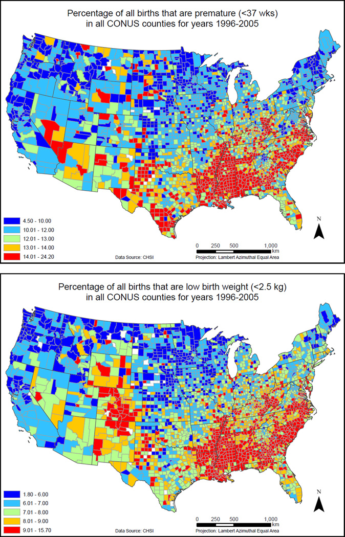
Currently, EXIS contains geospatial data sets for over 300 environmental, demographic, socioeconomic, and behavioral (EDB) attributes; these data sets cover the 3,109 contiguous U.S. (CONUS) counties at a spatial resolution that is typically at the census-tract level (but, depending on the attribute, may range from actual point locations to a county aggregate) and temporal resolutions that vary from hourly to annual. At a minimum, county-level maps (ArcGIS shapefiles) and summary statistics are provided for all these data sets in EXIS. In addition to variables corresponding to EDB attributes, data on selected health outcomes, potentially relevant to longitudinal birth cohort studies like the NCS, have also been incorporated in EXIS. For the examples presented here, three types of birth outcomes have been used for initial exploratory analysis: preterm birth (PB) rates (<37 weeks), low birth weight (LBW) (<2.5 kg), and very low birth weight (VLBW) (<1.5 kg, VLBW). Annual data for these outcomes are available for the period since 1996 from the Community Health Status Indicators project⁽³¹⁾ for 2,902 of the CONUS counties. Fig. 5 shows county-level maps for percentage rates of PB (top panel) and LBW (bottom panel).

Fig. 5.

Preterm birth rates and low birth weights were selected as representative health endpoints for the tier 1 and tier 2 exposure analyses presented in this work.

3.1. Tier 1 Analysis Examples

Objectives of the tier 1 exposure-relevant analyses within the TiER framework were to identify data gaps in EDB variables potentially associated with health outcomes, and to explore the representativeness of NCS attributes versus corresponding attributes of the U.S. population as a whole.

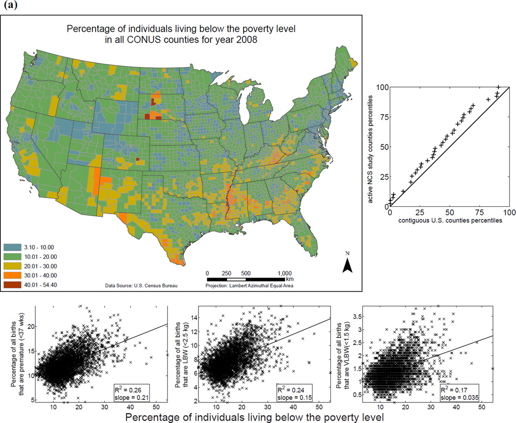
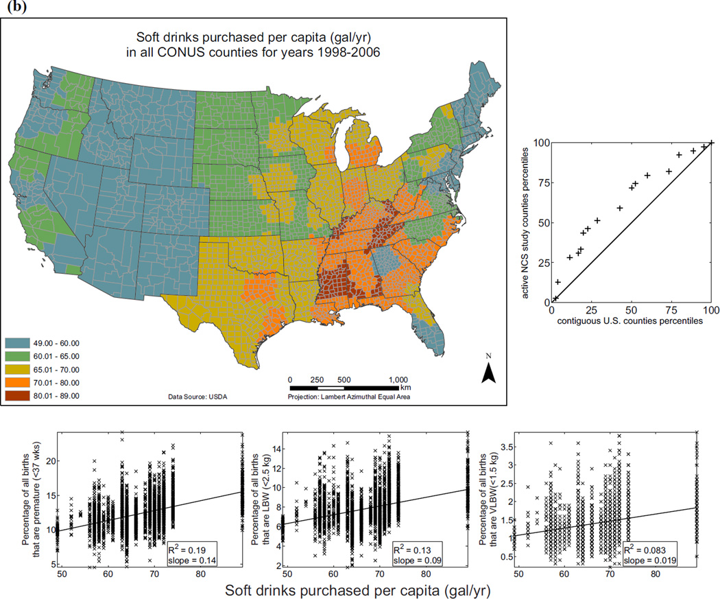
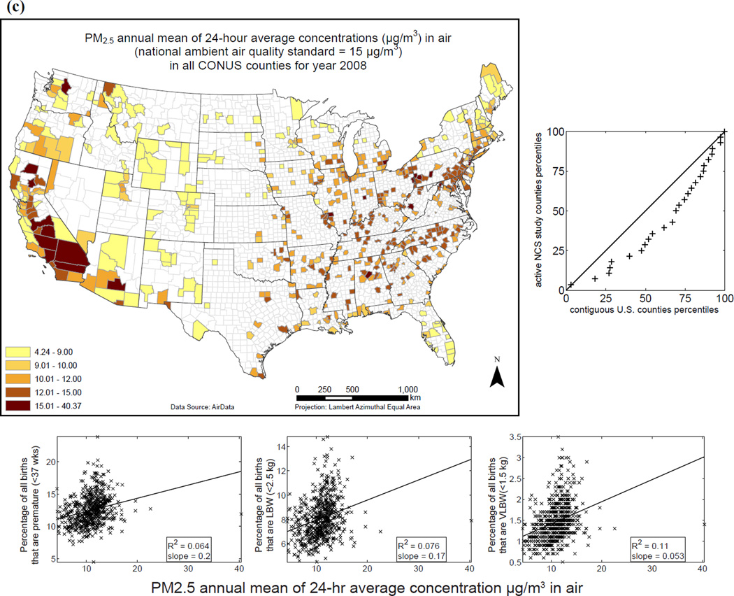
Examples of variables currently in EXIS are shown in Fig. 6 for: (i) distribution of individuals living below the poverty level (as percentage of county population) for 2008; (ii) soft drinks purchased per capita (annual average for years 1998–2006); and (iii) annual means of 24-hour ambient PM2.5 concentrations. The distributions of various exposure-relevant EDB attributes for the 40 current NCS counties versus all contiguous U.S. counties are compared via quantile-quantile (QQ) plots: the proximity of distribution quantile points to the 45° line is a measure of the similarity of the two distributions (Figs. 6(a), (b), and (c)). Variables are also visualized in scatterplots with linear (ordinary least squares) regression and logistic regression versus the selected endpoints of PB, LBW, and VLBW (Figs. 6(a), (b), and (c)).

Fig. 6.

Examples of exposure-relevant factors included in EXIS: (a) County-level map showing percentage of individuals living below the poverty level for 2008 in the CONUS.^(31,34) (b) County-level map showing soft drinks purchased per capita in the CONUS.^(31,35) (c) Annual average of ambient PM_2.5 levels observed in the CONUS in 2008.^(31,36) To the right of each map is a QQ plot: the proximity of distribution quantile points to the 45°; line as a measure of the similarity of the two distributions. Under each map are scatterplots showing linear (ordinary least squares) regression and logistic regression versus the selected endpoints of preterm birth (PB), low birth weight (LBW), and very low birth weight (VLBW).

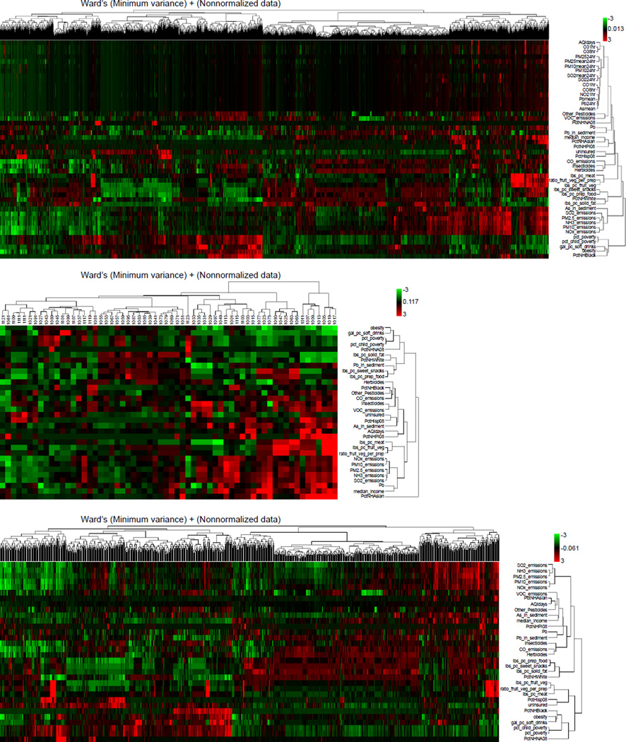
Patterns of association for a representative set of EDB variables were explored in relation to the three selected birth outcomes. The 2,902 CONUS counties for which data for all three outcomes were available were classified into the six urban/rural categories defined by the National Center for Health Statistics.⁽³²⁾ Then, the birth outcome data sets and the selected EDB data for these 2,902 counties were analyzed using two variants of the biclustering method: (i) the two-way hierarchical clustering analysis tool in ebTrack/ArrayTrack and (ii) the clustergram function in Matlab. Both tools use hierarchical clustering with Euclidean distance and average linkage options. The data were clustered sequentially by counties first and then by EDB variables, resulting in the heatmap of Fig. 7(a). Many counties did not have available measured values for the environmental quality variables. These gaps are identifiable as a black area on the heatmap. The heatmap was then subdivided according to the urban/rural classifications defined by the National Center for Health Statistics in order to compare the patterns of variables for these “generalized environments” (Figs. 7(b) and (c)). The heatmap provides an approach for examining patterns of potentially NCS-relevant data across all CONUS counties as well as separately for rural/urban counties: it depicts locations where there are data gaps, as well as locations where strong associations among variables of concern may exist.

Fig. 7.

Biclustered heatmaps showing similarities between selected exposure-relevant attributes for (a) the 2,902 CONUS counties for which data are available for all three birth outcomes (PB, LBW, and VLBW) considered in this analysis; (b) for 62 “central” counties containing a metropolitan area with population >1 million; and (c) for 1,216 “noncore” counties (i.e., counties that are neither micropolitan nor metropolitan, with urban population of up to 19,999 adjacent to a metropolitan area or with urban population of up to 49,999 not adjacent to a metropolitan area).

In Figs. 7(b) and (c), the data were divided by county type into two groups: in Fig. 7(b), the 62 “central” metro area counties with population >1 million and in Fig. 7(c), the 1,216 “noncore” counties with urban population <49,999 not adjacent to a metro area or <19,999 adjacent to a metro area. The same clusters appear in the heatmaps split by urban/rural designation as in the heatmap of all CONUS counties. The results suggest some national similarities that can be examined further using extant data at the segment level for individual counties.

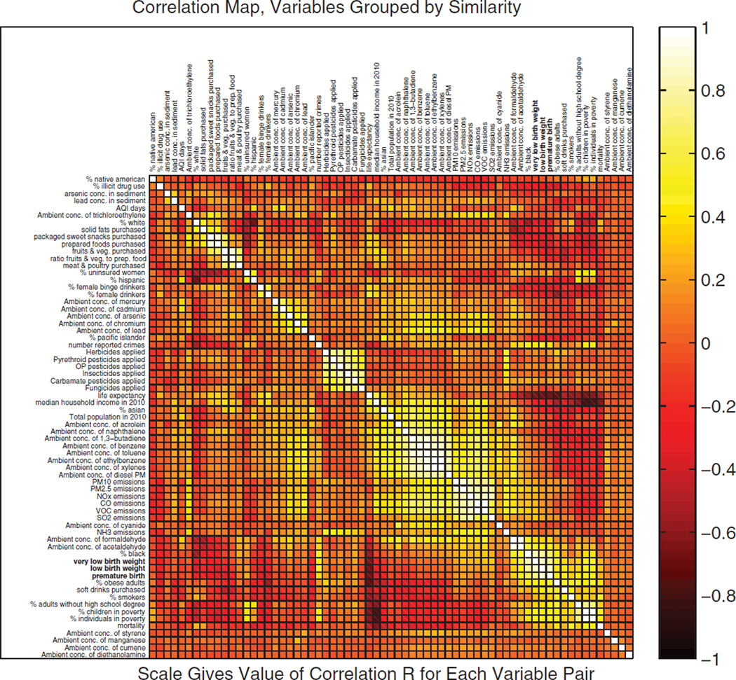
Subsequently, a correlation matrix was generated to examine the linear dependence between various pairs of exposure-relevant EDB variables in EXIS. Fig. 8 shows a correlation map with variables that have been “ordered” by k-nearest neighbors clustering. Of the 2,415 pairs of exposure-relevant variables 109 (4.5%) have a correlation coefficient greater than 0.6. As expected, strong correlations exist between variables from the same data “categories”: e.g., two highly correlated environmental variables are the emissions of CO and VOCs (r = 0.97), both typically linked to motor vehicle operation. Examples of demographic/socioeconomic variables that have high correlation with the selected health endpoint of LBW are life expectancy (r = −0.68) and the percentage of population that is non-Hispanic black (r = 0.77). Another interesting relationship occurs with obesity, which is correlated with life expectancy (r = −0.70) and moderately correlated with gallons of soft drinks purchased per capita (r = 0.55) and percentage of premature births (r = 0.53). These observations reinforce the need to consider multiple variables or representative surrogates in environmental health studies such as the NCS. Additionally, it would be useful to have periodic updates in examining such correlation matrices, to help understand changes in values of selected variables during child growth and development.

Fig. 8.

Exploratory multivariate analysis of exposure-relevant factors (included in EXIS) with respect to selected birth outcomes: the correlation map is a visual representation of the linear dependence between pairs of variables (which are grouped here by similarity). The analysis has been performed with county-level data for the CONUS.

3.2. Tier 2 Demonstration Case Study: Inhalation EIs for Birth Outcomes

Tier 2 analyses within the TiER framework have focused primarily on the calculation of risk-related EIs, both at the county level across the NCS, and at the segment level for Queens County, NY (see Isukapalli et al.⁽¹³⁾). The first exposure route considered for the EI analyses was inhalation, and the first health endpoints considered in relation to inhalation exposure were PB and LBW. As mentioned above, inflammation was hypothesized as a plausible BMOA for linking the endpoints with relevant variables in order to formulate the appropriate risk-relevant EI (Fig. 4). The endpoints (PB and LBW rates) were selected in consultation with the NCS Program Office; however, the consideration of the particular BMOA is not restrictive, and it is used here to provide a reasonable example for EI definition.

A total of 48 air pollutants, i.e., 4 criteria pollutants and 42 air toxics (listed in Table I) with established (noncancer) respiratory effects were used in formulating the algorithm for the calculation of PB and LBW risk-relevant inhalation EIs, employing a Monte Carlo approach. Of course, as stated earlier, these are not the only—or the most important—factors associated with inflammation, but they are used to provide an example application of the approach. Specifics of the formulation are outlined below.

Table I.

Airborne Contaminants Used in Formulating the Inhalation Exposure Index for Premature Birth (PB) and Low Birth Weight (LBW) Risks Along with the (Noncancer) Toxicity Reference Concentrations (from USEPA⁽⁷⁾)

Chemical Name of Air Pollutant	CAS Number	Reference Concentrations (RfCs)(mg/m3 Unless Indicated Otherwise)
Criteria pollutants
Ozone (O3)	10028-15-6	30 ppm (summer season average)
Nitrogen dioxide (NO2)	10102-44-0	0.015
Sulfur dioxide (SO2)	94336-28-4	53 ppb
Fine particulate matter (PM2.5)	NA	30 ppb
Air toxics
Acetaldehyde	75070	0.009
Acrolein	107028	0.00002
Acrylic acid	79107	0.001
Acrylonitrile	107131	0.002
Antimony compounds	7440360	0.0002
Beryllium compounds	7440417	0.00002
Bis(2-ethylhexyl)phthalate	117817	0.01
Chlorine	7782505	0.00015
2-Chloroacetophenone	532274	0.00003
Chloroprene	126998	0.007
Chromium compounds	18540299	0.0001
Cobalt compounds	7440484	0.0001
1,3-Dichloropropene	542756	0.02
Diesel particulate matter	N/A	5
Diethanolamine	111422	0.003
Epichlorohydrin	106898	0.001
1,2-Epoxybutane	106887	0.02
Ethylene dibromide (Dibromomethane)	106934	0.009
Ethylene glycol	107211	0.4
Formaldehyde	50000	0.0098
Hexachlorocyclopentadiene	77474	0.0002
Hexamethylene-1,6-diisocyanate	822060	0.00001
Hydrochloric acid	7647010	0.02
Maleic anhydride	108316	0.0007
Methyl bromide (bromomethane)	74839	0.005
Methyl isocyanate	624839	0.001
Methyl methacrylate	80626	0.7
4,4′-Methylene diphenyl diisocyanate (MDI)	101688	0.0006
Naphthalene	91203	0.003
Nickel compounds	7440020	0.00009
Nitrobenzene	98953	0.009
Phosgene	75445	0.0003
Phthalic anhydride	85449	0.02
Propionaldehyde	123386	0.008
Propylene dichloride	78875	0.004
Propylene oxide	75569	0.03
Styrene oxide	96093	0.02
Titanium tetrachloride	7550450	0.0001
Toluene	108883	5
2,4-Toluene diisocyanate	584849	0.00007
Triethylamine	121448	0.007
Vinyl acetate	108054	0.2

A representation of the EI calculation algorithm specific to inhalation exposure is provided in the following equation:

$$E_{\text{inhalation},i,p}=[{\omega }_{\text{toxics},p}\sum _{j=1}^{N_{\text{toxics},p}}\frac{\overline{C_{i,j}}}{Rf{C}_{j,p}}+{\omega }_{\text{crit},p}\sum _{k=1}^{N_{\mathit{\text{crit}},p}}(\frac{{\int }_{{\tau }_1}^{{\tau }_2}{C}_{i,k}(t)dt}{({\tau }_2-{\tau }_1)}\times \frac{1}{Rp{C}_{k,p}({\tau }_2,{\tau }_1)}\left)\right]\times {\omega }_{\text{pop},i,p},$$

where:

Einhalation, i, p	inhalation EI for area i in relation to endpoint p
i	geographic area of concern (e.g., segment or county)
p	endpoint of concern (e.g., respiratory and inflammation effects)
$\overline{C_{i,j}}$	average concentration of the air toxic j in area i
Ci, k(t)	concentration of criteria pollutant k in area i at time t
τ1 and τ2	start and end of averaging period for concentrations of criteria pollutant k in area i
ωtoxics, p	relative weight of air toxics in relation to health endpoint p
ωcrit, p	relative weight of criteria pollutants considered in relation to endpoint p
ωpop, i, p	target population weight of area i in relation to endpoint p (e.g., fraction of female population of child-bearing age)
Ntoxics, p	number of air toxics considered in relation to endpoint p
Ncrit, p	number of criteria pollutants considered in relation to endpoint p
RfCj, p	reference concentration for air toxic j in relation to endpoint p
RpCk, p(τ1, τ2)	a reference concentration for criteria pollutant k in relation to endpoint p for averaging period between τ 1 and τ 2

In general, each area of interest (“NCS location”) will have subareas with varying pollutant levels; for example, if the area of study is a county, substantial variability in air pollutant levels is expected to exist within the county. Even in the case of individual NCS segments, such variability occurs because each segment may include blocks from multiple census tracts, each with varying environmental quality and demographics.

The computational implementation of the EI formulation utilizes Monte Carlo methods to incorporate this variability, via the following steps:

1. Generation of a set of samples for each population group within each subarea of a study area (e.g., 100 samples for each person in the target population subgroup). By aggregating these samples, spatial variations in population distributions are taken into consideration.

2. For each sampled individual, assignment of inhalation rate based on representative distributions of inhalation rates for the specific age-gender combination and the inhalation and aggregate potential intakes.

3. Normalizing these estimates through a reference inhalation rate (e.g., average inhalation rate for the population subgroup) and reference concentration.

These estimates provide distributions of EI estimates at the resolution of the study area (segments or counties).

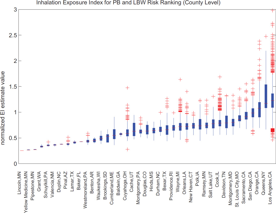
Calculated estimates of county-level inhalation EI ranges are shown as box plots in Fig. 9 for each of the 40 “active” NCS counties. The box plots illustrate the presence of gradients in the EI within each county. The edges of the box plots in the graphs show the 25th (q1) and 75th (q3) percentiles. The whiskers are 1.5 times the interquartile range (q3 − q1) corresponding to approximately +/− 2.7σ and 99.3% coverage when the data are normally distributed. The whisker is extended to the most extreme data point that is not an outlier; outliers are plotted as plus signs (assuming a normal distribution). The results show the range and variability of EI values across current NCS counties: the two counties with the highest means and ranges of estimated EI values are Queens, NY, and Los Angeles, CA.

Fig. 9.

Estimates of “county-level” ambient inhalation exposure index formulated in relation to birth outcomes (such as preterm birth and low birth weight) for the 40 active NCS locations.

4. DISCUSSION AND CONCLUSIONS

Characterization of maternal, prenatal, and early childhood exposures to environmental pollutants across all routes and pathways, including diet and consumer product usage, are important components of the NCS. Collecting data on many environmental variables for the assessments will, of necessity, require a combination of measurements taken in the home and possibly the neighborhood of participants, and of measurements taken routinely by a variety of agencies and organizations. The 40 “active” NCS counties were the subject of this study-wide application of the TiER framework: the results suggest that these NCS counties are generally representative of the nation for the variables studied, and that there are many associations of exposure factors, not only environmental, but also—and often primarily— socioeconomic and behavioral, that should be explored in the future in relation to the health end-points considered.

Development of risk-relevant EIs for the inhalation exposure route was proven feasible with extant data at the national level for each NCS county, but presents various challenges. For example, data can be very heterogeneous (in quality, technical specifications, etc.) and data variability can be significant within a demographic unit or with regard to seasonal, weekly, or diurnal patterns. However, at least at the county level, such data are sufficient to support “lower-tier” characterization and rankings of exposures across the NCS.

Ongoing work is focusing on the systematic study of the relationships between predicted EIs that were estimated for diverse locations and the relevant health outcomes for these locations.

Other ongoing and planned environmental health modeling applications of the TiER framework also consider explicitly exposures at the individual level, using specific home and personal data. These applications incorporate “reverse modeling”⁽¹⁹⁾ to take advantage of biomonitoring data, “personalized” behavioral and activity information, and individual-specific microenvironmental dynamics. TiER, in conjunction with EXIS, offers a systematic approach for addressing the challenges associated with this effort by allowing integration of diverse-relevant information (from genetic to physiological to behavioral, etc.) for performing individual-and population-based modeling in a manner that takes explicitly into account intra- and inter-individual variability.

REFERENCES

- 1.National Academies. The exposome: A powerful approach for evaluating environmental exposures and their influences on human disease. Emerging Science for Environmental Health Decisions. 2010 Jun [Google Scholar]
- 2.NIH. Summary of the NIH Genes, Environment, and Health Initiative (GEI) Workshop on Gene-Environment Interplay in Common Complex Diseases. Presented at NCS Environmental Summit; Bethesda, MD. 2010. [Google Scholar]
- 3.Rappaport SM. Implications of the exposome for exposure science. Journal of Exposure Science and Environmental Epidemiology. 2011;21(1):5–9. doi: 10.1038/jes.2010.50. [DOI] [PubMed] [Google Scholar]
- 4.Lioy PJ, Rappaport SM. Exposure science and the exposome: An opportunity for coherence in the environmental health sciences. Environmental Health Perspectives. 2011;119:a466–a467. doi: 10.1289/ehp.1104387. [DOI] [PMC free article] [PubMed] [Google Scholar]
- 5.Putzrath RM, Wilson JD. Fundamentals of health risk assessment. Use, derivation, validity and limitations of safety indices. Risk Analysis. 1999;19(2):231–247. doi: 10.1023/a:1006973627307. [DOI] [PubMed] [Google Scholar]
- 6.Feron V, Van Vliet P, Notten W. Exposure to combinations of substances: A system for assessing health risks. Environmental Toxicology and Pharmacology. 2004;18:215–222. doi: 10.1016/j.etap.2003.11.009. [DOI] [PubMed] [Google Scholar]
- 7.USEPA. Prepared by ICF International for the US Environmental Protection Agency. North Carolina NC: Durham; 2011. [Accessed October 29, 2013]. An Overview of Methods for EPA’s National-Scale Air Toxics Assessment. Available at: http://www.epa.gov/airtoxics/nata2005/05pdf/nata_tmd.pdf. [Google Scholar]
- 8.Sarigiannis D, Hansen U. Considering the cumulative risk of mixtures of chemicals — A challenge for policy makers. Environmental Health. 2012;11(Suppl 1):S18. doi: 10.1186/1476-069X-11-S1-S18. [DOI] [PMC free article] [PubMed] [Google Scholar]
- 9.USEPA. Washington, DC: US Environmental Protection Agency; 2012. [Accessed October 29, 2013]. Risk Assessment Guidance for Superfund (RAGS) Part A – Chapter 8: Risk Characterization. Available at: http://www.epa.gov/oswer/riskassessment/ragsa/pdf/ch8.pdf. [Google Scholar]
- 10.Marshall S, Gennings C, Teuschler LK, Stork LG, Tornero-Velez R, Crofton KM, Rice GE. An empirical approach to sufficient similarity: Combining exposure data and mixtures toxicology data. Risk Analysis. 2013;33(9):1582–1595. doi: 10.1111/risa.12015. [DOI] [PMC free article] [PubMed] [Google Scholar]
- 11.Lioy PJ, Isukapalli S, Trasande L, Thorpe L, Dellarco M, Weisel C, Georgopoulos PG, Yung C, Brown M, Landrigan P. Using national and local extant data to characterize environmental exposures in the National Children’s Study (NCS): Queens County. 10. Vol. 117. New York: Environmental Health Perspectives; 2009. pp. 1494–1504. [DOI] [PMC free article] [PubMed] [Google Scholar]
- 12.Hirschfeld S, Kramer B, Guttmacher A. Current status of the National Children’s Study. Epidemiology. 2010;21(5):605–606. doi: 10.1097/EDE.0b013e3181ea603b. [DOI] [PubMed] [Google Scholar]
- 13.Isukapalli S, Brinkerhoff CJ, Dellarco M, Landrigan PJ, Lioy PJ, Georgopoulos PG. Exposure indices for the National Children’s Study: Application to inhalation exposures in Queens County, NY. Journal of Exposure Science and Environmental Epidemiology. 2013;23:22–31. doi: 10.1038/jes.2012.99. [DOI] [PMC free article] [PubMed] [Google Scholar]
- 14.Georgopoulos PG, Isukapalli S, Lioy P. PRoTEGE–A three-tier system that supports exposure-based prioritization of chemicals. Presented at USEPA Exposure-Based Chemical Prioritization Workshop; September 26–27, 2011; Research Triangle Park, NC. 2011. [Google Scholar]
- 15.Mitchell J, Arnot JA, Jolliet O, Georgopoulos P, Isukapalli S, Dasgupta S, Pandian M, Wambaugh J, Egeghy P, Cohen-Hubal EA, Vallero DA. Comparison of modeling approaches to prioritize chemicals based on estimates of exposure and exposure potential. Science of the Total Environment. 2013;458–460:555–567. doi: 10.1016/j.scitotenv.2013.04.051. [DOI] [PMC free article] [PubMed] [Google Scholar]
- 16.Georgopoulos PG, Wang SW, Vyas VM, Sun Q, Burke J, Vedantham R, McCurdy T, Ozkaynak H. A source-to-dose assessment of population exposures to fine PM and ozone in Philadelphia, PA, during a summer 1999 episode. Journal of Exposure Analysis and Environmental Epidemiology. 2005;15(5):439–457. doi: 10.1038/sj.jea.7500422. [DOI] [PubMed] [Google Scholar]
- 17.Georgopoulos PG, Lioy PJ. From a theoretical framework of human exposure and dose assessment to computational system implementation: The Modeling Environment for Total Risk studies (MENTOR) Journal of Toxicology and Environmental Health – Part B, Critical Reviews. 2006;9(6):457–483. doi: 10.1080/10937400600755929. [DOI] [PubMed] [Google Scholar]
- 18.Georgopoulos P. A multiscale approach for assessing the interactions of environmental and biological systems in a holistic health risk assessment framework. Water, Air, Soil Pollution: Focus. 2008;8(1):3–21. [Google Scholar]
- 19.Georgopoulos PG, Sasso AF, Isukapalli SS, Lioy PJ, Vallero DA, Okino M, Reiter L. Reconstructing population exposures to environmental chemicals from biomarkers: Challenges and opportunities. Journal of Exposure Science and Environmental Epidemiology. 2009;19(2):149–171. doi: 10.1038/jes.2008.9. [DOI] [PMC free article] [PubMed] [Google Scholar]
- 20.Xue J, Zartarian V, Wang SW, Liu SV, Georgopoulos PG. Probabilistic modeling of dietary arsenic exposure and dose and validation with 2003 NHANES data. Environmental Health Perspectives. 2010;118(3):345–350. doi: 10.1289/ehp.0901205. [DOI] [PMC free article] [PubMed] [Google Scholar]
- 21.Brand KP, Small MJ. Updating uncertainty in an integrated risk assessment: Conceptual framework and methods. Risk Analysis. 1995;15(6):719–729. [Google Scholar]
- 22.Isukapalli SS, Roy A, Georgopoulos PG. Stochastic Response Surface Methods (SRSMs) for uncertainty propagation: Application to environmental and biological systems. Risk Analysis. 1998;18(3):351–363. doi: 10.1111/j.1539-6924.1998.tb01301.x. [DOI] [PubMed] [Google Scholar]
- 23.Isukapalli S, Roy A, Georgopoulos PG. Efficient sensitivity/uncertainty analysis using the combined Stochastic Response Surface Method (SRSM) and Automatic Differentiation for FORTRAN code (ADIFOR): Application to environmental and biological systems. Risk Analysis. 2000;20:591–602. doi: 10.1111/0272-4332.205054. [DOI] [PubMed] [Google Scholar]
- 24.Isukapalli S, Spendiff M, Georgopoulos PG, Krishnan K. Uncertainty, variability and sensitivity analyses in simulation models. In: Krishnan K, Andersen ME, editors. Quantitative Modeling in Toxicology. Chichester, UK: John Wiley; 2010. pp. 429–458. [Google Scholar]
- 25.Georgopoulos PG, Wang SW, Lioy PJ, Georgopoulos IG, Yononne-Lioy MJ. Assessment of human exposure to copper: A case study using the NHEXAS database. Journal of Exposure Science and Environmental Epidemiology. 2006;16:397–409. doi: 10.1038/sj.jea.7500462. [DOI] [PubMed] [Google Scholar]
- 26.Chen M, Martin J, Fang H, Isukapalli S, Georgopoulos PG, Welsh WJ, Tong W. ebTrack: An environmental bioinformatics system built upon ArrayTrack. BMC Proceedings. 2009;3(Suppl 2):S5. doi: 10.1186/1753-6561-3-s2-s5. [DOI] [PMC free article] [PubMed] [Google Scholar]
- 27.Tong W, Cao X, Harris S, Sun H, Fang H, Fuscoe J, Harris A, Hong H, Xie Q, Perkins R, Shi L, Casciano D. ArrayTrack–supporting toxicogenomic research at the USFDA-NCTR. Environmental Health Perspectives. 2003;111(15):1819–1826. doi: 10.1289/ehp.6497. [DOI] [PMC free article] [PubMed] [Google Scholar]
- 28.Georgopoulos PG, Isukapalli SS, Burke J, Napelenok S, Palma T, Langstaff J, Majeed M, He S, Byun D, Cohen M, Vautard R. Air quality modeling needs for exposure assessment from the source-to-outcome perspective. Environmental Manager. 2009:26–35. [Google Scholar]
- 29.USEPA. Consolidated Human Activity Database 2009. [Accessed October 29, 2013]; Available at: http://www.epa.gov/chadnet1/
- 30.USEPA. 2005 National Emissions Inventory (NEI) 2008. [Accessed October 29, 2013]; Available at: http://www.epa.gov/ttnchie1/net/2005inventory.html.
- 31.US DHHS. Community Health Status Indicators (CHSI) Project 2009. [Accessed October 29, 2013]; Available at: http://communityhealth.hhs.gov.
- 32.CDC. National Center for Health Statistics (NCHS) 2006. [Accessed October 29, 2013]; Available at: http://www.cdc.gov/nchs.
- 33.Behrman RE, Butler AS. Preterm Birth: Causes, Consequences and Prevention. Washington, DC: Institute of Medicine; 2007. [Accessed October 29, 2013]. Available at: http://www.nap.edu/catalog.php?record_id=11622. [Google Scholar]
- 34.USCB. US Census for 2000 projected for 2008. [Accessed October 29, 2013];2000 Available at: http://www.census.gov.
- 35.USDA. Food Environment Atlas Data from 1998–2006. [Accessed October 29, 2013];2010 Available at: http://ers.usda.gov/foodatlas/
- 36.USEPA. AirData — Access to monitored air quality data from EPA’s Air Quality System (AQS) Data Mart. [Accessed October 29, 2013];2012 Available at: http://www.epa.gov/airdata/
Associated Data
This section collects any data citations, data availability statements, or supplementary materials included in this article.