Testing Genetic Association by Regressing Genotype over Multiple Phenotypes

Abstract

Complex disorders are typically characterized by multiple phenotypes. Analyzing these phenotypes jointly is expected to be more powerful than dealing with one of them at a time. A recent approach (O'Reilly et al. 2012) is to regress the genotype at a SNP marker on multiple phenotypes and apply the proportional odds model. In the current research, we introduce an explicit expression for the score test statistic and its non-centrality parameter that determines its power. Same simulation studies as those reported in Galesloot et al. (2014) were conducted to assess its performance. We demonstrate by theoretical arguments and simulation studies that, despite its potential usefulness for multiple phenotypes, the proportional odds model method can be less powerful than regular methods for univariate traits. We also introduce an implementation of the proposed score statistic in an R package named iGasso.

Introduction

Complex human disorders are often characterized by multiple phenotypes. Some of them might be categorical while others might be continuous. For instance, patients with Bardet-Biedl syndrome often suffer from vision loss, hypertension and high cholesterol level caused by obesity, polydactyly, and other abnormalities. In order to map the genetic variants underlying such disorders, it is highly desirable to analyze all available phenotypes simultaneously. However, it is challenging to jointly model these phenotypes, especially when they are of different data types [1].

Let denote a vector of phenotypes on an individual and his/her genotype at a marker. If all the components of are continuous, one may use MANOVA given genetype . When the components of are of mixed data types, the choices are limited. One popular method is to first analyze each component individually and then combine the test statistics through a meta-analysis [2], [3]. These methods model the phenotype vector in terms of the genetic data .

For a single-nucleotide polymorphism (SNP), the distribution of its genotype is trinomial. It is appealing to model as a function of [4], [5]. Furthermore, since there is a natural ordering in the three genotypes at the SNP (assuming that the possibility of over-dominance is ignorable), one can use the ordinal logistic regression (a.k.a., the proportional odds model or the cumulative logit model) [6]. One immediate advantage of using the proportional odds model is that, unlike other methods, there is no need to make assumptions on the genetic effect such as additive, dominant, or recessive. The usefulness of this approach has been demonstrated via analyses of various data [5]. It is one of the best currently available multivariate methods [7]. However, it is the slowest one [7].

The test used in [5] is the likelihood ratio test (LRT). It involves numerical maximization under both the null hypothesis and the alternative hypothesis. We introduce a score test statistic using standard statistics theory. This statistic is asymptotically equivalent to the likelihood ratio test but computationally much faster due to the availability of its explicit expression, a feature useful in genome-wide association analysis. This explicit expression also gives insight on how the proportional odds model works in the context of genetic association analysis.

This report is organized as follows. We first introduce an explicit form of the score statistic and its non-centrality parameter. The form of this score statistic provides some insights on the ability of this method to detect association. The performance of the this score statistic is evaluated using the same simulation scenarios used in [7]. Finally, we consider an important case where the phenotype vector is univariate and binary to see how this test works for univariate phenotypes.

Results

The score statistic

The genetic data are assumed to come from a biallelic marker such as a single-nucleotide polymorphism (SNP). Let denote the reference allele and the other. For simplicity, we use 0, 1, and 2 to represent genotypes , , and , respectively. Regardless of the data types of the components of , the genotype follows a trinomial distribution. In most cases, the effect of an allele is monotonic. That is, as the number of alleles increases from 0 to 2, the effect of genotypes , , and is non-decreasing or non-increasing. Over-dominance effect exists but is rather rare. Given this consideration, we model the genotype in terms of phenotype using the proportional odds model [5].

Let denote the probability that an individual's genotype is given phenotypic value . In the current situation, the proportional odds model models the cumulative probabilities and jointly as follows:

(1)

(2)

Here and are intercepts and is a vector of coefficients. This model implies because . Since , an alternative form of equation (2) is

Equation (1) models the effect of phenotype y on the odds of genotype versus or while equation (2) models the effect of phenotype y on the odds of genotype versus or . We have

and is determined by . This model assumes that the difference of the left hand side of (1) or (2) for two phenotype vectors and depends only on and is independent of genotype or :

(3)

(4)

That is,

does not depend on the value of .

Let be the index for the th individual in a sample of size , the log-likelihood function is

The hypotheses of interest are

(5)

These hypotheses can be tested by the likelihood ratio statistic. To introduce the score statistic, define

where and are the sample proportions of the genotypes for which and 2, respectively. is the difference of two weighted summations of . The summation in the first pair of parentheses weights with more than other s (i.e., 1 versus ) while the summation in the second pair of parentheses weights with more (i.e., 1 versus ). Let . It is shown in the Methods section that a score statistic for testing hypotheses (5) is

where

is the sample variance matrix of . The non-centrality parameter of is

where the expectation in is taken under the alternative. This NCP can be used to compute power at significance level in the following way:

where follows a chi-square distribution with and non-centrality parameter and is the critical value from a chi-square distribution with and non-centrality parameter 0.

Simulation Study

The simulation study consists of two parts. In the first part, multivariate phenotypes were simulated the same way as in [7]. Genotype data at a single SNP were simulated with minor allele frequency under the assumption Hardy-Weinberg equilibrium. Three phenotypes, denoted by , and , were simulated using the following relationship:

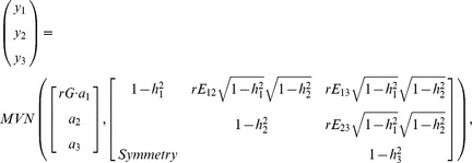where , , and are pre-spedfied residual correlations between phenotypes excluding the QTL effect, or controls the effect direction of (those of and are fixed at 1) and . Three scenarios were considered with only 1, 2, or all phenotypes were associated with the SNP. See [7] for more details. For each simulated data set, the LRT -value is obtained from the R package MultiPhen and the score -value is obtained from the R package iGasso. Empirical rejection rates over 1,000 replicates are reported in Table 1. The performance of the score test is very similar to that of LRT. The empirical power are very close to the power of LRT reported in [7].

Table 1. Non-centrality value and the associated power (presented in parentheses) for models used in the simulation studies.

	Frequency of Allele a	Effect of Allele a
K	p	Recessive	Additive	Dominant
0.01	0.1	—	4.6780 (0.2597)	14.4110 (0.8387)
	0.3	2.8697 (0.1329)	9.7282 (0.6225)	18.5977 (0.9339)
	0.4	6.9507 (0.4323)	—	—
0.1	0.1	—	5.7000 (0.3374)	17.6383 (0.9182)
	0.3	3.4771 (0.1730)	11.7847 (0.7343)	22.5123 (0.9737)
	0.4	8.4233 (0.5379)	—	—

The relative genotype risks are for recessive models; for dominant models; and for additive models.

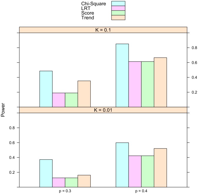
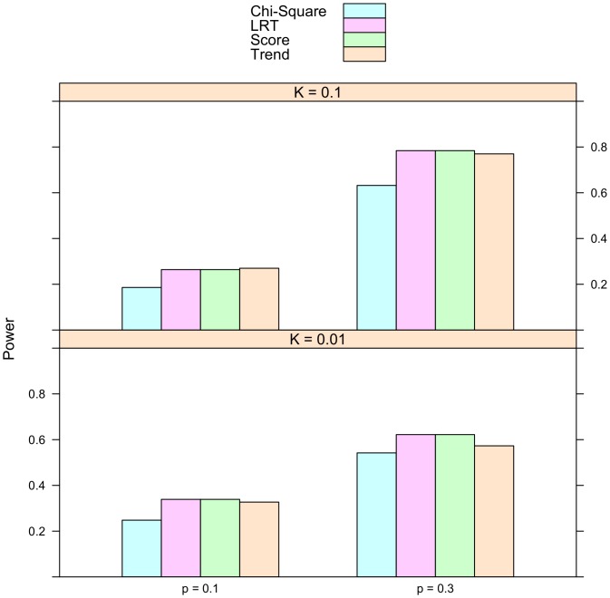
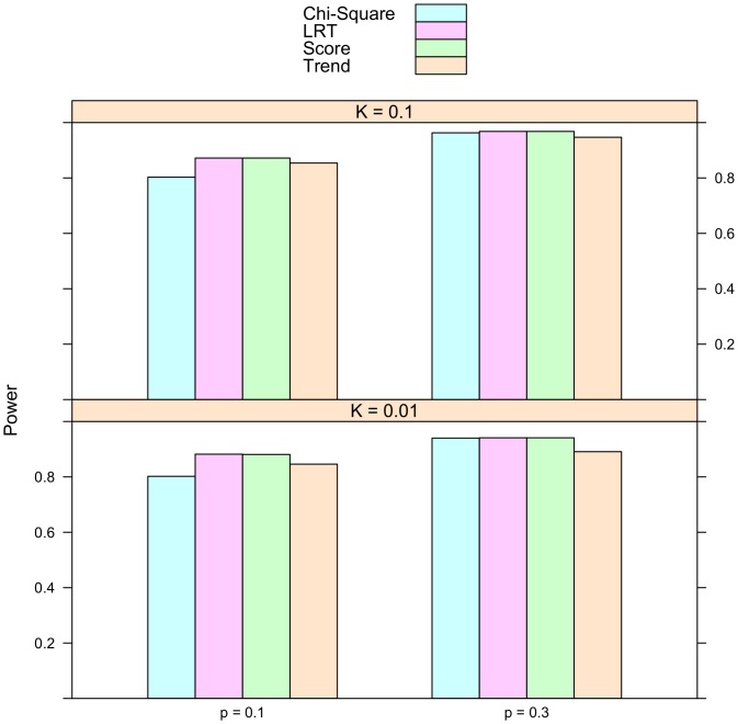
Is the proportional odds model always more powerful than the usual tests of association? To address this question, simulation were conducted on univariate phenotypes. The description of the simulation studies is provided in the Methods section. In addition to the proposed score statistic, the other test statistics used in the simulation include the Pearson's chi-square test, the Cochran-Armitage trend test, and the likelihood ratio test for the proportional odds model. The number of simulation replicates is fixed at 10,000. The sample size is 2,000. Half of the subjects are cases and half are controls. The simulated type I error rate for all these statistics is reported in Table 2. The empirical rejection rates are very close to their nominal levels, which are 0.1, 0.01, and 0.005. The simulated power is presented in Figures 1, 2, and 3. It is striking to see that for recessive models the proportional odds model is the least powerful. For instance, when prevalence and minor allele frequency , the power are 0.486 for Chi-Square test, 0.353 for Trend test, and 0.19 for both LRT and Score test. For other two models, there are situations it is more powerful than other methods. The simulated power for the statistic is in line with the calculated power reported in Table 3.

Table 2. Simulated type I error rate in the case of a univariate phenotype under various generating models.

Penetrance (K)	Frequency of Allele a (p)	Significance Level	Test Statistic
			Trend	Chi-Square	LRT	Score
0.01	0.1	0.1	0.085	0.095	0.091	0.091
		0.01	0.007	0.007	0.006	0.007
		0.005	0.005	0.004	0.004	0.004
	0.3	0.1	0.077	0.091	0.082	0.082
		0.01	0.009	0.008	0.010	0.010
		0.005	0.006	0.002	0.005	0.005
0.1	0.1	0.1	0.096	0.099	0.101	0.102
		0.01	0.011	0.009	0.010	0.010
		0.005	0.006	0.006	0.007	0.007
	0.3	0.1	0.116	0.117	0.109	0.108
		0.01	0.009	0.011	0.010	0.010
		0.005	0.006	0.007	0.003	0.003
0.01	0.1	0.1	0.085	0.095	0.091	0.091
		0.01	0.007	0.007	0.006	0.007
		0.005	0.005	0.004	0.004	0.004
	0.3	0.1	0.077	0.091	0.082	0.082
		0.01	0.009	0.008	0.010	0.010
		0.005	0.006	0.002	0.005	0.005
0.1	0.1	0.1	0.096	0.099	0.101	0.102
		0.01	0.011	0.009	0.010	0.010
		0.005	0.006	0.006	0.007	0.007
	0.3	0.1	0.116	0.117	0.109	0.108
		0.01	0.009	0.011	0.010	0.010
		0.005	0.006	0.007	0.003	0.003
0.01	0.1	0.1	0.085	0.095	0.091	0.091
		0.01	0.007	0.007	0.006	0.007
		0.005	0.005	0.004	0.004	0.004
	0.3	0.1	0.077	0.091	0.082	0.082
		0.01	0.009	0.008	0.010	0.010
		0.005	0.006	0.002	0.005	0.005
0.1	0.1	0.1	0.096	0.099	0.101	0.102
		0.01	0.011	0.009	0.010	0.010
		0.005	0.006	0.006	0.007	0.007
	0.3	0.1	0.116	0.117	0.109	0.108
		0.01	0.009	0.011	0.010	0.010
		0.005	0.006	0.007	0.003	0.003

The test statistics are: Trend — Cochran-Armitage trend test; Chi-Square — Pearson's chi-square test; LRT — the likelihood ratio test for the proportional odds model computed by using the polr function in the R package MASS; Score — the proposed score statistic computed by using the SNPass.test function in the R package iGasso.

Figure 1. Simulated power for recessive model.

The relative genotype risks are . K represents disease prevalence and p is the frequency of allele a. The abbreviations for the test statistics are the same as in Table 2.

Figure 2. Simulated power for additive model.

The relative genotype risks are . K represents disease prevalence and p is the frequency of allele a. The abbreviations for the test statistics are the same as in Table 2.

Figure 3. Simulated power for dominant model.

The relative genotype risks are . K represents disease prevalence and p is the frequency of allele a. The abbreviations for the test statistics are the same as in Table 2.

Table 3. Simulated power under the same simulation scenarios of [7] over 1,000 replicates.

			Scenario
			I		II		III
rG	rE	MAF q	LRT	Score	LRT	Score	LRT	Score
1	0.0	0.01	0.125	0.125	0.184	0.183	0.278	0.278
		0.40	0.141	0.141	0.198	0.197	0.257	0.257
	0.3	0.01	0.127	0.129	0.185	0.185	0.184	0.183
		0.40	0.124	0.123	0.177	0.178	0.187	0.185
	0.7	0.01	0.221	0.221	0.268	0.267	0.129	0.129
		0.40	0.215	0.211	0.292	0.292	0.138	0.136
−1	0.0	0.01	—	—	0.202	0.201	0.289	0.288
		0.40	—	—	0.194	0.192	0.269	0.262
	0.3	0.01	—	—	0.267	0.266	0.344	0.344
		0.40	—	—	0.277	0.273	0.351	0.354
	0.7	0.01	—	—	0.589	0.589	0.694	0.694
		0.40	—	—	0.548	0.542	0.717	0.713

In scenario I, only phenotype 1 is associated with the SNP. rG = 1 or −1 does not affect the simulation results. Only results with rG = 1 are shown.

Discussion

In this report, we introduced a score test statistic for the proportional odds model for testing the association between a SNP and multiple phenotypes and provided an implementation of this statistic. Same simulation studies as those reported in [7] were conducted to assess it performance. We also did simulation analyses to study the performance of proportional odds model for univariate phenotypes which is covered by [5]. Although appealing to studies on multiple phenotypes, this method may be less powerful for univariate traits than regular methods. For case-control data, our results suggest that the traditional Pearson's chi-square test and the Cochran-Armitage trend test are preferred when the disease allele frequency is less than 0.5 and the disease is recessive.

Nonetheless, the proportional odds model method provides a convenient way for analyzing multiple phenotypes, especially when these phenotypes are of different types [5]. If the proportional odds assumption is of concern, one may remove this assumption and adopt a multinomial logistic regression. For our simulation studies, the multinomial logistic regression would be equivalent to the Pearson's chi-square test statistic. There are quite few implementations of the multinomial logistic regression, for instance, the multinom function in R package nnet.

Methods

Derivation of the score statistic

The first-order derivatives of the log-likelihood function are

and the second-order derivatives are

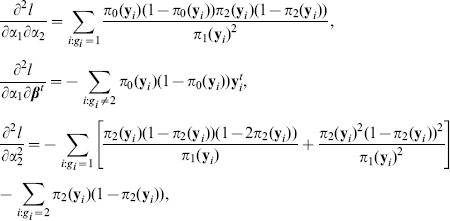Under , no longer depends on . So their values are simply denoted by , and , respectively. Let . The expected Fisher information matrix evaluated at is

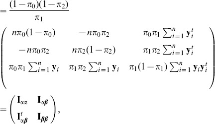where the matrix partition is in an obvious manner. By standard asymptotic theory, the score statistic is

where is evaluated at :

The unknown values of , and are estimated by their sample genotype proportions, respectively.

Simulation Studies

Here is a description of the simulation procedure for the case of a dichotomous phenotype. Suppose the trait is Mendelian. Let , , and denote the frequencies of genotypes , and in general population and , , and their penetrances, respectively. The prevalence of the disease would be . The genotype frequencies in cases are and in controls are . In this situation, the variance of is where is the proportion of cases. The non-centrality parameter (NCP) of test statistic is equal to

Let be the population frequency of allele a. Assuming Hardy-Weinberg equilibrium in the population, the frequencies of genotypes , , and are , and , respectively. Let , be the relative risk of genotype to genotype 0. A data generating model is completely determined by , , , and . This is because , , and . Hence the genotype frequencies in cases and controls are determined and data can be simulated. We consider a dominance model (), a recessive model (), and an additive model (). The NCPs for the models used in simulation are reported in Table 3. So are the power associated with these NCPs.

R function SNPass.test

The R function SNPass.test in the package iGasso implements the proposed score statistic. R users can download and install iGasso from CRAN (http://cran.r-project.org/) or any CRAN mirror.

Data Availability

The author confirms that all data underlying the findings are fully available without restriction. The statistical test proposed in the manuscript has been implemented in R language. It is freely available at http://cran.r-project.org/web/packages/iGasso/index.html. The R code is available upon request from the corresponding author.

Funding Statement

This research is funded by the National Institute for Environmental Health Sciences through the University of Iowa Environmental Health Sciences Research Center, NIEHS/NIH P30 ES05605. The funder has no role in study design, data collection and analysis, decision to publish, or preparation of the manuscript.

References

- 1. Zhu W, Zhang H (2009) Why do we test multiple traits in genetic association studies. Journal of the Korean Statistical Society 38: 1–10. [DOI] [PMC free article] [PubMed] [Google Scholar]
- 2. Xu X, Lu Tian L (2003) Combining dependent tests for linkage or association across multiple phenotypic traits. Biostatistics 4: 223–229. [DOI] [PubMed] [Google Scholar]
- 3. Yang Q, Wu H, Guo CY, Fox CS (2010) Analyze multivariate phenotypes in genetic association studies by combining univariate association tests. Genet Epidemiol 34: 444–454. [DOI] [PMC free article] [PubMed] [Google Scholar]
- 4. Wang K, Huang J (2011) Treating phenotype as given: A simple resampling method for genome-wide association studies. Genetic Analysis Workshop 17 5: S60. [DOI] [PMC free article] [PubMed] [Google Scholar]
- 5. O'Reilly PF, Hoggart CJ, Pomyen Y, Calboli FCF, Elliott P, et al. (2012) MultiPhen: Joint model of multiple phenotypes can increase discovery in GWAS. PLoS ONE 7: e34861. [DOI] [PMC free article] [PubMed] [Google Scholar]
- 6.Agresti A (2002) Categorical Data Analysis. John Wiley & Sons, Inc., 2nd edition.
- 7. Galesloot TE, van Steen K, Kiemeney LALM, Janss LL, Vermeulen SH (2014) A comparison of multivariate genome-wide association methods. PLoS ONE 9: e95923. [DOI] [PMC free article] [PubMed] [Google Scholar]
Associated Data
This section collects any data citations, data availability statements, or supplementary materials included in this article.
Data Availability Statement