Abstract
Voxel-based analysis is widely used for quantitative analysis of brain MRI. While this type of analysis provides the highest granularity level of spatial information (i.e., each voxel), the sheer number of voxels and noisy information from each voxel often lead to low sensitivity for detection of abnormalities. To ameliorate this issue, granularity reduction is commonly performed by applying isotropic spatial filtering. This study proposes a systematic reduction of the spatial information using ontology-based hierarchical structural relationships. The 254 brain structures were first defined in multiple (n=29) geriatric atlases. The multiple atlases were then applied to T1-weighted MR images of each subject data for automated brain parcellation and five levels of ontological relationships were established, which further reduced the spatial dimension to as few as 11 structures. At each ontology level, the amount of atrophy was evaluated, providing a unique view of low-granularity analysis. This reduction of spatial information allowed us to investigate the anatomical features of each patient demonstrated in an Alzheimer’s disease group.
Introduction
Analysis of images from multiple subjects necessitates that, first and foremost, anatomically corresponding structures are identified across the subjects. The region-of-interest (ROI) approach, in which specific target structures, such as the hippocampus, are manually defined, is the most widely used approach and is considered to be the gold standard in the field of quantitative neuroanatomy. This approach however, is time-consuming and is applicable only to a small portion of anatomical structures. For example, with a 1 mm isotropic spatial resolution, a brain with a 1.2 L volume would have 1.2 million voxels. The hippocampus volume is typically about 4,000 voxels (4 ml), meaning only 0.3% of the voxels are evaluated. An alternative approach is voxel-based analysis, in which correspondence is established automatically across all 1.2 million voxels between the two brains (see e.g., [1]). Suppose we have 50 control and 50 patient images. The entire dataset can be expressed as two matrices of [(50 subjects) × (1.2 million voxels)]Control, Patient. This voxel-vector (of 1.2 million voxels) needs to be re-ordered, such that any arbitrary vector element, say, the ith voxel of the 1.2 million-element vector, identifies the same anatomical locations across the 100 subjects. Then, we can contract the 50-element population dimension to the average and the standard deviations; the two matrices are now [(average, standard deviation) × (1.2 million voxels)]. The actual measurements could be voxel intensity (e.g., T2, fractional anisotropy, mean diffusivity) or morphometric parameters representing local atrophy or hypertrophy (e.g., Jacobian). This contraction now enables us to perform a t-test at each voxel, identifying voxels with significantly different values between the two populations.
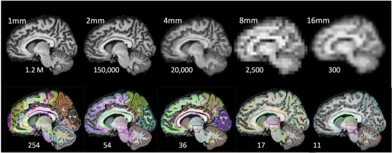
Voxel-based analysis is powerful because it retains the maximum amount of location information until the final statistical analysis; the entire brain is examined at the highest granularity level, i.e., 1.2 million voxels. However, the limitations of this approach are also widely recognized (see e.g., [2]). First of all, the information each voxel carries is noisy. This issue is magnified by that fact that there are 1.2 million intricately dependent observations. Second, the accuracy of voxel-based registration is not guaranteed (the 1.2 million voxel-vectors may not be well-aligned across subjects). This lack of accuracy can be attributed to two sources: 1) lack of contrast—the voxel-to-voxel mapping between two corresponding regions is not accurate if the regions lack contrast; and 2) anatomical heterogeneity—excessive anatomical variability in certain areas, such as cortical folding, could prevent us from accurately identifying corresponding voxels between two brains in such areas. To ameliorate the issue of noise, we typically reduce the level of granularity by applying a uniform spatial filter, effectively reducing the image resolution through voxel averaging (Fig. 1).
Fig. 1.
Comparison of granularity reduction by isotropic resolution reduction (upper row) and ontology-based structural reduction (bottom row).
In this study, we provide tools to analyze the 50 × 1,200,000 matrices using an alternative approach. In many clinical studies, even if the patient population is as homogenized as possible by stringent clinical criteria, a considerable amount of anatomical, and, potentially, pathological heterogeneity remains. Our primary interest is, therefore, to characterize the anatomical heterogeneity within a patient group. Different patients may have abnormalities in different locations. If so, our interest is the first subject dimension (e.g., n = 50) of the matrices, and the group-aggregated statistics (reduction of the average and standard deviation) at each location are no longer appropriate for analysis. This naturally leads us to an alternative concept, which is the reduction of the second dimension (n = 1,200,000). In VBA, this is achieved by spatial filtering. While this is an effective approach, the level of granularity remains high (2,300) even with an 83 reduction of voxel size, and considerable amount of anatomical information is lost. To address these issues, we used an alternative approach, in which voxels are not grouped uniformly according to spatial proximity, but rather, based on pre-defined anatomical criteria called atlases.
This anatomy-specific filtering based on a pre-defined atlas, however, has several issues. First, the number of defined structures is limited by available image contrasts. T1-based contrast could define up to several hundred structures. If there are 300 defined structures, each structure has, on average 4,000 voxels. Compared to VBA, the level of granularity is substantially low, potentially making the measurement insensitive to highly localized abnormalities. Second, there are multiple criteria by which to define structures, and, depending on pathology, different criteria may be used. For example, for vascular diseases, brain parcellation based on the vascular territories may make more sense than classical ontology-based brain parcellation. Third, the accuracy issues of the VBA due to the lack of the contrasts and cross-subject variability still exist for the structure-based analysis, although they may influence the results in different ways. Once the voxels are grouped to define a structure, the location information of each voxel inside the structure degenerates and there is no longer a voxel-wise accuracy issue. Instead, it manifests as the accuracy of the boundary definition
In this study, we developed a tool that can flexibly change the granularity level based on the hierarchical relationships of 254 structures defined in our atlas. We tested this tool within the framework of a multiple-atlas brain parcellation algorithm [3-9]. Using 29 pre-parcellated atlases, test data were automatically parcellated into the smallest structural units (254 structures). Then, these structures were dynamically combined at five different hierarchical levels, down to 11 structures [10, 11]. This provides a flexible view to evaluate brain anatomy at multiple granularity levels. This tool was first applied to a control group to measure test-retest reproducibility and normal range of anatomical variability. Then, we analyzed Alzheimer’s disease (AD) patients for demonstration purposes.
Methods
Subjects
Three study groups were used for this study: young adult controls; elderly controls; AD patients. All studies were approved by the Institutional Review Board of Johns Hopkins University and written, informed consent was obtained from all patients.
Young adult subjects
A database for normal adult subjects was obtained from previous studies (n = 17, mean age = 31 years old, age range 22 to 49 years old) [12], in which each subject was scanned twice, two weeks apart. Scan parameters were MPRAGE, matrix 256×256, FOV 256mm×256mm, slice thickness 1.2mm, TE 3.15ms, and TR 6.747ms. These data were used to measure the test-retest precision of the method and anatomical variability within the young normal subjects.
Alzheimer’s disease (AD) patients and elderly controls
We used AD and elderly data from a study of a well-characterized group of individuals conducted by the Johns Hopkins Alzheimer’s Disease Research Center (ADRC), with written, informed consent in accordance with the requirements of the Johns Hopkins Institutional Review Board and the guidelines endorsed by the Alzheimer’s Disease Association [13]. Detailed demographic, health, clinical features, and initial findings have been reported previously [14]. Briefly, the study sample comprised 8 patients (mean age, 75.6) who met NINCDS/ADRDA criteria for AD [15] and had a Clinical Dementia Rating (CDR) of 1, and 10 individuals (mean age, 74.3) who were cognitively normal and had a CDR=0 (normal controls or NC). The demographic characteristics of the subjects were as follows: AD—mean age = 75.6, mean education = 15.7, male/female = 5/3; and NC—mean age = 74.3, mean education = 16.2, male/female = 3/7. Subjects were excluded from enrollment if they were under the age of 55, had a history of a neurological disease other than AD, or a history of major psychiatric illness. As previously described [14], there were no differences among these groups with regard to age, sex, race, education, and the occurrence of vascular conditions, such as hypertension, hypercholesterolemia, and heart attack. Written, informed consent was obtained under the oversight of the Johns Hopkins Institutional Review Board using guidelines of the Alzheimer’s Disease Association [13]. MPRAGE scans were conducted according to the protocol of the Alzheimer’s Disease Neuroimaging Initiative (ADNI) [16], with an echo time of 3.2 ms and a repetition time of 6.9 ms. The imaging matrix was 256 × 256, with a field of view of 240 × 240 mm, zero-filled to 256 × 256 mm, and a sagittal slice thickness of 1.2 mm.
Atlas inventory
In this study, we used multiple atlases (JHU T1 Geriatric Multi-Atlas Inventory) to perform automated brain parcellation. This atlas inventory is designed for geriatric patient populations with potential brain atrophy. The atlas data were based on a portion of the AD/elderly population described above, specifically, AD patients (n = 15, age mean = 73 years old, age range 56 to 80 years old) and normal elderly controls (n = 14, age mean = 75 years old, age range 60 to 80 years old). To create the multi-atlas inventory, our JHU single-subject brain atlas (Eve atlas) [17-19] was initially warped to the 29 multiple atlases using a method described by Djamanakova et al. [20], followed by manual corrections for mislabels. The resulting images were parcellated into 254 structures defined in the JHU brain atlas.
Image processing
The multiple-atlas brain parcellation was performed using the following steps on the test/control subjects:
All T1-WIs were bias-corrected and skull-stripped using SPM5 (The Wellcome Dept. of Imaging Neuroscience, London; www.fil.ion.ucl.ac.uk/spm). After initial linear alignment, all atlases were warped to the subject image using Large Deformation Diffeomorphic Metric Mapping (LDDMM) [19, 21, 22]. The transformation matrix was then applied to the co-registered parcellation maps of each atlas. The details of the multi-atlas fusion algorithm used in this study are described in our previous publication [24]. Briefly, let A be a set of given atlas-label pairs, A = {(Ia,Wa)}, where Ia denotes the gray-scaled T1-WI of the atlas-label pair a, and Wa denotes the corresponding manual segmentations of Ia. Given a to-be-segmented subject, I, we model the distribution of the intensity in each region-of-interest (ROI) in the subject image as a conditional Gaussian random field, conditioned on the unknown atlas-label pair and the ROI-specific unknown diffeomorphism. The algorithm for segmentation iterates between the selection of the atlas-label pair and the construction of locally optimized diffeomorphisms as a variant of the expectation-maximization (EM) method. Define the Q-function as the conditional expectation of the complete-data log-likelihood, given the incomplete-data and the previous segmentation estimation, according to:
where the sum is obtained over all voxels, x, in the image domain, and over the atlas-label pairs, a. The sequence of estimated segmentations, W(1), W(2), …, is updated by the iteration:
whose calculation is alternated with the calculations of the conditional probabilities, PA(x)(a|I, Wold). PA(x)(a|I, Wold) is derived from the conditional mean of the indicator function, and encodes the set of atlas-label pairs being selected in the interpretation [23].
Ontology-based multi-granularity analysis using RoiEditor:MriStudio
All analyses were performed using the final parcellations in the native space of the subjects. The 254 structures defined in the parcellation map were assigned a hierarchical relationship based on their ontological relationship. This relationship consists of five hierarchical levels. As the level goes up, the granularity of structural definition increases as following: 11 - 17 - 36 – 54 - 254. This relationship was implemented in RoiEditor (X. Li, H. Jiang, and S. Mori, Johns Hopkins University, www.mristudio.org), as shown in Fig. 1. As the brain is parcellated into multi-level structures, the sizes of all structures are calculated automatically using this software. It is important to note that only one parcellation was performed for each subject, at the highest granularity level. The subsequent reparcellation to different granularity levels was achieved by the recombination of individual ROIs to create new, larger ROIs. The hierarchical relationship of the structures in the 5 granularity levels as defined by the authors is available for download at https://www.mristudio.org/wiki/installation. The hierarchical relationship can also be user-defined through the text file.
Test-retest measurements of multi-atlas segmentation
To assess the test-retest reproducibility of the whole-brain, multi-atlas parcellation method, the data from the twice-scanned young adult subjects (n=17) were utilized. The volume data were compared for all regions of each subject across the two scans. From this dataset, the test-retest reproducibility for each subject was measured. In addition, anatomical variability among the 17 normal subjects was measured. The test-retest measurement precision and the anatomical variability were then compared using a principal component analysis.
Characterization of anatomical features of AD patients
To characterize the anatomical features of AD patients, multi-atlas segmentation was performed on all patients, and the multi-granularity-level analysis was performed. The anatomical features of each patient were presented by z-scores based on the age-matched control data.
Results
Test-retest variability
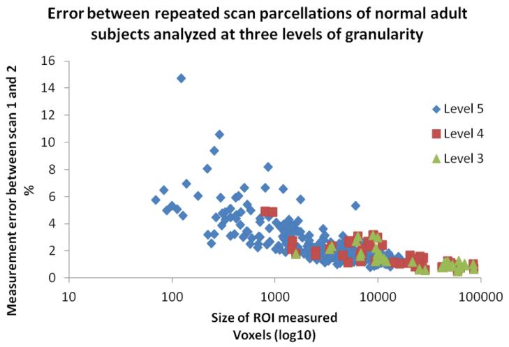
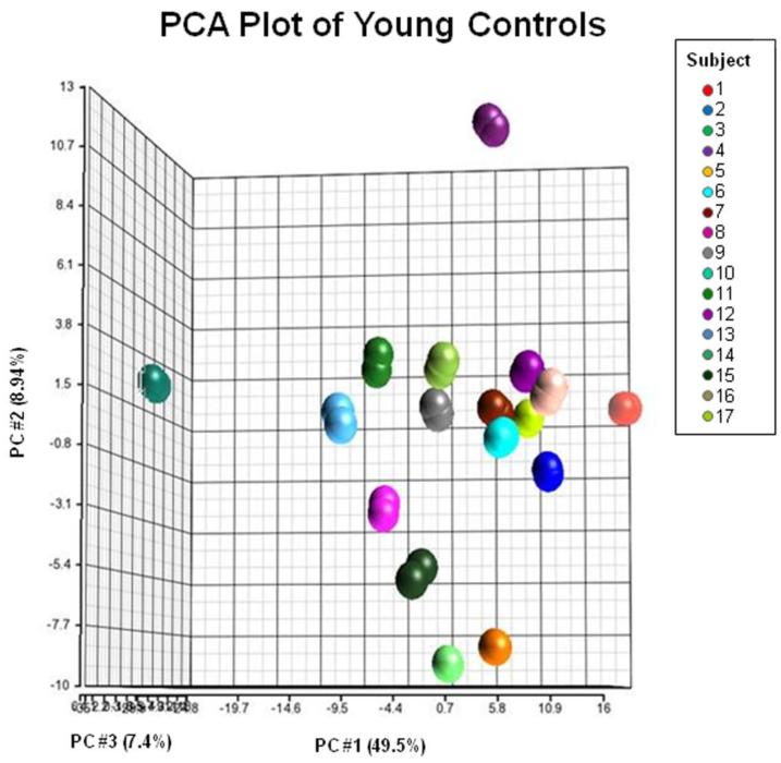
The test-retest variability (percent volume difference) across all ROIs between the two scans was found to be 2.6% ± 1.7%, 1.7% ± 1%, 1.4% ± .7%, 1.5% ± 0.7%, and 1.5% ± 0.9% for the five different granularity levels (highest to lowest level). Fig. 2 shows the relationship between the variability and the size of the parcellation at three different granularity levels (Level 3, 4, and 5). A clear inverse relation can be seen, in which the variability increases drastically for structures less than 1,000 voxels, while most of the structures larger than 1,000 voxels have a small amount of variability (< 2%). At Level 4, there are only two structures that are less than 1,000 voxels in size and none in Level 1-3. Consequently, the improvement in the average test-retest variability for Level 1-4 was negligible. Figure 3 shows the results of principal component analysis (PCA) using the 254 ROIs in the highest granularity level. The plot based on the first three principal components clearly isolates anatomical features of the 17 normal subjects, with respect to the test-retest variability, suggesting the test-retest precision of this approach is high enough to characterize anatomical features of the normal population.
Fig. 2.
Plot of test-retest analysis using 17 healthy subjects, scanned twice. The variability between scan 1 and 2 is plotted as a percent of ROI size for each ROI measured at three highest granularity levels. The x-axis is the size of the structures in voxels (log10).
Fig. 3.
PCA results of the test-retest analysis using 17 healthy subjects, scanned twice. The data are plotted against the first three principal components, maximizing the separation of the data. There are two data points for each subject indicated. Colors correspond to different subjects. Axes represent principal components that account for the most variability between the 34 data points. Each principal component is a linear combination of the 254 parcels.
Anatomical variation among the normal subjects
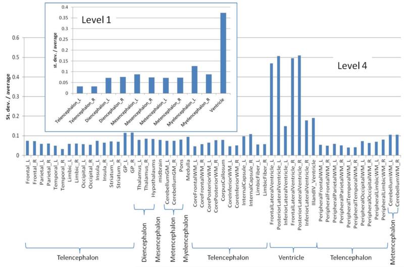
Fig. 4 shows the anatomical variability at two different granularity levels (level 1 and 4) of segmentation for the young normal adults. A few things to note are: 1) the lateral ventricles are the most variable features within normal adult populations, given that the average level of variability is at ~40%; and 2) as the level of granularity increases (and thus, each defined structure becomes smaller), the variability tends to increase, which could be the result of a combination of true anatomical variability and reduction of parcellation accuracy. For example, in level 1, the left telencephalon shows a variability of 2.6% in the normal population. At level 2, regions that comprise the left telencephalon are the left cerebral cortex, the cortical nuclei, and the white matter. Their average variability was 4.0%. Further breaking down these regions into smaller sub-regions (i.e., the cortex is divided into the frontal, parietal, temporal, limbic, and occipital cortices) at level 3, the average variability at this level is 5.8%. This indicates the trade-off between finer localization information and measurement precision. We can expect that the higher granularity levels, in general, provide more information about the shape variability. For example, the level 4 data suggest that the large population variability of the ventricle volume seen in level 1 is mostly due to the large variability of the anterior and posterior lateral ventricles, while the third and fourth ventricles have much less variability.
Fig. 4.
Coefficients of variance for the volumes of measured structures from the 17 normal subjects at two different granularity levels: level 1 (11 structures) and level 4 (54 structures). A complete ontology table can be found at https://www.mristudio.org/wiki/installation.
Comparison of AD and age-matched control groups
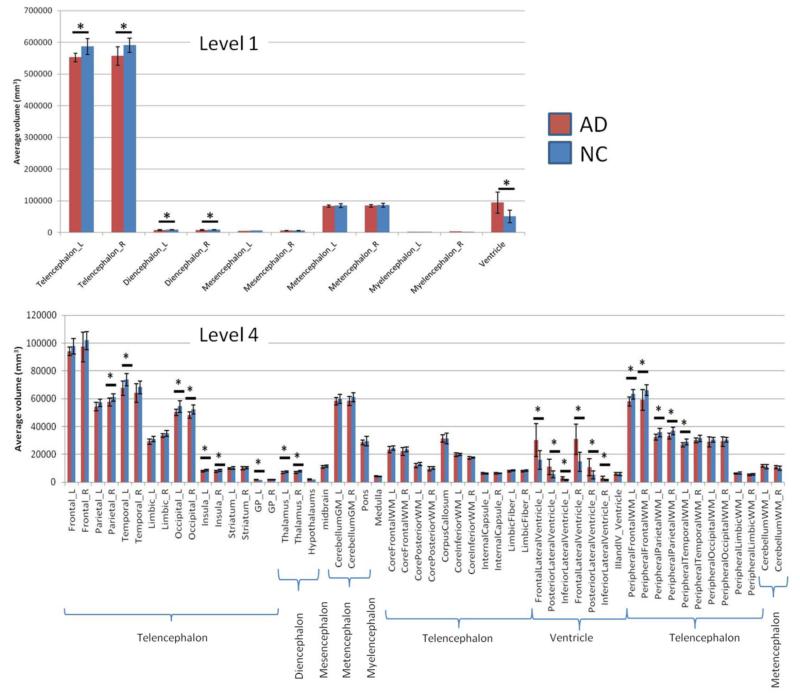
Fig. 5 shows the “classical” view of anatomical abnormalities in an AD population. The graphs show that, at the lowest granularity level, a statistically significant difference was found at the ventricles (hypertrophy) and telencephalon and diencephalon (atrophy) between the AD and NC populations. As the granularity level increases, a more detailed view of the tissue atrophy can be obtained. At level 4, 20 structures reached statistical significance (p<0.05) between the two groups. However, after a Bonferroni multiple comparison correction, none of the regions from levels 3-5 were significantly different at α < 0.05.
Fig. 5.
Comparison of volumes of the brain structures defined in level 1 and level 4 between AD patients and age-matched control subjects. Statistical tests were based on a t-test without multiple comparison correction.
Individual views of anatomical features
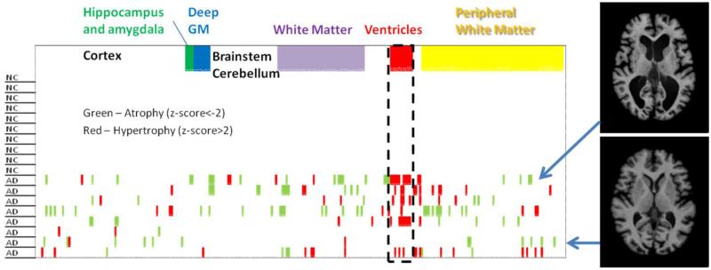
Fig. 6 shows an alternative view of the same AD data at level 5, in which the within-group data contraction (e.g., population averaging) was not performed and the anatomical feature of each individual was delineated using z-scores. In this analysis, we first calculated the average and standard deviations of the volume of each structure from the age-matched controls, and then, the z-scores were calculated for each AD patient. As expected, none of the structures in the control group reached a z-score higher than 2 (or less than −2). On the other hand, many “relatively” atrophic (indicated by pink) and hypertrophic (indicated by green) structures existed in the AD group. For example, the ventricles stand out as regions where many AD patients deviate substantially from the normal mean. However, even with our AD population, with stringent inclusion criteria, the spatial distributions of atrophic areas varied widely among the eight AD patients, which can be visually appreciated from the two example cases shown in Fig. 6. The structure-by-structure population averaging used in Fig. 5 could lead to: 1) the loss of patient-specific anatomical features; and 2) lower sensitivity due to the inclusion of patients with abnormalities at different anatomical locations. Fig. 7 shows an example of image-based representation of a multi-granularity analysis result, in which the z-score of each defined structure is color-coded in a parcellated patient image.
Fig. 6.
A “barcode” view of the population data for the 10 normal controls and eight AD patients. For each of the 254 defined structures at level 5, a z-score was calculated based on the normal control data. The structures with less than (pink) or more than (green) two standard deviations from the normal values are indicated. Insert: Images of two representative AD cases are shown.
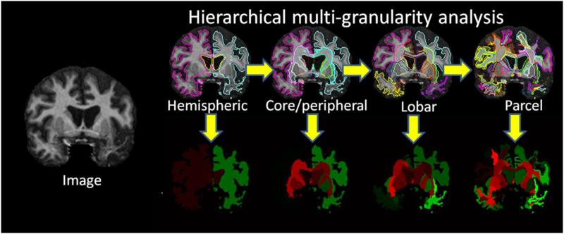
Fig. 7.
Illustration shows an image-based view of the multi-granularity analysis as it would be calculated in RoiEditor. In practice, z-scores calculated in Fig. 6 would be used for color coding. Green – relatively smaller region compared to a control group. Pink – relatively larger region compared to a control group.
Discussion
Tradeoff between granularity and variability
The measurements of test-retest reproducibility of our automated brain parcellation using a multi-atlas approach indicated that the measurement precision was high, with respect to anatomical variability, among the normal subjects (Fig. 3). The test-retest precision became lower as the granularity increased, and at the highest granularity level, the reproducibility was 2.6 +/− 1.7% for all 254 measured structures. There was also a tendency for the amount of anatomical variability among the young normal subjects to increase as the granularity increased (Fig. 4). This was probably due to the mixture of real anatomical variability and a decreased level of measurement precision.
In PCA (Fig. 3), we calculate total variance of two measurements of the 17 subjects. This variance contains scanning reproducibility (test-retest), automated segmentation errors, cross-subject variability, and other sources of variability. PCA attempts to find sources of variability in the measurements and determines three most dominant sources, which, in this case, accounts for 65.9 % of the total variance. The three axes are the combination of measured structures and thus do not have immediate anatomical meaning. What is important is the two repeated measurements were naturally clustered in the PCA space with respect to the cross-subject variability. Therefore, we can conclude that reproducibility of the automated quantification method is high compared to expected amount of cross-subject variability.
The multi-granularity analysis was also applied to a well-characterized AD population and an age-matched control group. Our study sample size was too small to draw a solid conclusion about AD pathology, but there were several interesting findings. First, as expected from the test-retest reproducibility and the anatomical variability among the normal population, the statistical power to detect the group difference decreases as the granularity increases. The lower granularity analysis did detect statistical differences after multiple-comparison correction, but the findings lacked spatial details about the pathology; for example, the level 1 analysis simply told us that the AD population had brain tissue atrophy and enlarged ventricles. On the other hand, if hypothesis-driven measurements of, for example, hippocampal volumes of an AD population suggest 10% volume loss and, simultaneously, our low-granularity analysis suggests 10% volume loss of the entire gray matter, the conclusion that “hippocampal volume is different in AD population compared to the control population” may be misleading because it singles out one structure as opposed to the entire gray matter. Thus it is important to analyze not only structures of interest, but also their substructures, and greater areas to which the structures belong. Observing MR data from multiple granularity levels and investigating spatial specificity is, thus, important. From the same T1 data sets, different granularity levels offer multiple options to analyze the data with different statistical power and different levels of anatomical specificity. From the sensitivity point of view, one could argue the sensitivity of analysis is at the highest when the granularity level matches the spatial extent of the abnormality; we may lose the sensitivity when the defined structures are too large (and thus, would include non-affected regions) or too small (the atrophic areas would be divided into too many regions).
Brain parcellation criteria
The above argument leads to a fundamental question about all parcellation-based image analysis: “are we parcellating the brain with proper anatomical criteria?” For example, we know that the distribution of ischemic areas follows vasculature territories, but not the tissue type. If our interest is to find the affected vasculatures, the atlas we employed, which is based on tissue types, is not appropriate. And if we want to identify brain structures and associated functions that are affected by an infarction, a parcellation scheme that represents brain functional distribution would be needed.
The multi-granularity parcellation scheme we offer in this paper is based on the brain ontology used in the atlas by Mai et al. [10], as well as by the Allen Brain Institute (http://human.brain-map.org/). Here, our assumption is that the evolutionarily-conserved, ontology-based anatomical definition is the most suitable way to represent brain anatomy and functions. However, there are multiple ontology definitions in the brain, and, thus, our scheme cannot be considered a gold standard. In fact, our ontology may not be compatible with the structural definitions with which we are most familiar. For example, in radiological descriptions, the brainstem is typically divided into the midbrain, the pons, and the medulla. However, classical ontology divides it into the mesencephalon, metencephalon, and myelencephalon, in which the mesencephalon includes the pons and the cerebellum together. In many ataxia patients, atrophy occurs in the pons and the cerebellum together, and, for a low granularity analysis, the classical ontology-based analysis could be more appropriate. As such, there is certainly a large amount of latitude in defining the hierarchical relationships of the brain structures.
There are several important issues related to this topic. When we define ontology-based atlases, the criteria used to parcellate the brain and the way we define hierarchical relationships are two different issues. The former could lead to multiple structural definitions that are mutually exclusive. For example, the same brain could be parcellated based on tissue type, vasculature territories, cytoarchitectures, or distribution of specific receptors, etc. The latter is a question of how to combine structures defined in the higher granularity levels (in our case, 254 structures) and establish a hierarchical relationship. For the latter issue, RoiEditor provides a flexible interface to incorporate user-defined hierarchical relationships through an ontology table.
The latter is also possible if users have their own brain parcellation maps. However, while the latter issue (how to combine structures and build an ontology relationship) is purely an issue of image analysis after the image parcellation at the highest granularity is complete, the former issue is related to how we should parcellate the image to begin with. This issue is discussed more in detail in the next section.
One interesting question is what defines the highest granularity level. Why doesn’t our parcellation map contain more than 254 structures? The parcellation is generally driven by available image contrast, but it is not an exact science and arbitrary judgment is involved. For example, even though we know that the hippocampus consists of many substructures, the hippocampus is defined as one structure. This is because we lack both resolution and contrast to sub-divide the hippocampus using conventional MRI of live human subjects. Indeed, because our parcellation map was created based on multiple contrasts (T1, T2, and DTI) [18, 19, 24], there are certain structures that are delineated in the atlas, but are invisible in T1-weighted images. One such structure, the pons, is divided into the middle cerebellar peduncle, the corticospinal tract, and the medial lemniscus, which are clearly identifiable on DTI but not on T1 images. In this case, T1-weighted imaging may not be able to detect atrophy specific to the corticospinal tract. This level of structural granularity is reliable in DTI, but it may not be reliable for T1. Therefore, the use and interpretation of the multi-level granularity analysis requires anatomical knowledge.
Multi-atlas approach
In this study, we employed our multi-atlas brain parcellation approach, called Diffeomorphic Probability Fusion (DPF) [23], because we have found that it is generally more accurate than a single-atlas approach. However, both approaches operate under the same concept: 1) all voxels of the atlases are mapped to the corresponding voxels in a patient, based on image transformation; 2) the brain structures are defined in the atlases as a “parcellation map;” and 3) the parcellation maps are then transferred to the patient using the transformation results from step #1. If we have only one atlas, this is a single-atlas approach. If we have multiple atlases, multiple parcellation maps are cast to a patient brain and a fusion process is required to combine the multiple maps [3-9]. Our ontology-based analysis is independent of how the brain is parcellated and can be used with either parcellation approach.
In the previous section, the issue of brain parcellation criteria was discussed. For example, we have four different types of parcellation maps in our single-subject atlas called the “Eve Atlas” (www.mristudio.org): the tissue type map used in this study; a vasculature map; a resting-state functional connectivity map; and a cytoarchitectonic map [19, 24-26]. If a single-atlas approach is used, the application of these different brain parcellation criteria is straightforward; we simply need to apply the transformation matrix to any parcellation maps of interest and warp the maps to the patient data. This concept can also be easily applied to the multi-atlas approach, but, practically speaking, preparing multiple atlases with multiple parcellation maps is a time-consuming step that requires an extensive amount of manual work.
Individualized analysis
The biggest motivating factor to use low-granularity analysis, as opposed to voxel-based analysis, is that the large reduction of spatial information from 1.2 million voxels to a mere 11-254 structures allows us to evaluate anatomical features of individual patients, as shown in Fig. 6. In high-granularity analysis, such as voxel-based analysis, a common approach is to contract the population dimension and average all patient information for each individual voxel. This approach increases the statistical power when the entire population shares the abnormality at similar locations. Our preliminary analysis of the AD population, however, even with stringent inclusion criteria, revealed highly heterogeneous anatomical features (Fig. 6). We believe that the reduction of spatial information is a key for individualized image analysis for clinical diagnosis. The task of this ontology-based analysis is to compress the 1.2 million voxel spatial dimension, while losing a minimum amount of pathology information. This is an essential step, if we want to combine MRI-based anatomical features with non-image clinical information, such as demography, lifestyle, clinical symptoms, lab tests, etc., to improve our ability to stratify the heterogeneous patient groups or predict the outcomes [25].
This paper is not intended to claim the superiority of individual-based analyses over group-based methods. In fact, the two methods are used for different purposes. Population-based analysis remains the better approach to analyze, for example, therapeutic effects. The tools for individual-based approaches are probably more suitable to support clinical practices. For example, z-score maps could supplement image reading (Fig. 7) and an individual’s atrophy pattern could be used to search past similar cases. Our study, however, did not prove the clinical usefulness of our approach for individualized image analyses. What is lacking is the knowledge database that can support the interpretation of certain anatomical features and link them to clinical covariate, such as long-term outcomes. In the PCA-type analysis, the population data are not reduced to population-representative numbers and an individual’s data could be correlated to the population data. This type of analysis, combined with a large knowledge database, is likely to be a key for future studies to effectively use past anatomical information to enrich the clinical decision-making process.
Conclusion
In this study, we introduced the concept of low-granularity anatomical analysis, which relies on ontology-based hierarchical relationships of brain structures. We combined this method with a multi-atlas parcellation approach and applied it to T1-weighted brain MRI to perform a comprehensive full brain atrophy analysis. The test-retest reproducibility of the multi-atlas parcellation approach was high. Using the combined approach, the anatomical variability of the normal population was measured at five different granularity levels as an estimate of power calculation. This approach was then applied to AD populations. The potential of this approach to perform individually-based anatomical analysis was discussed. The proposed approach was integrated into RoiEditor to allow for fully automated, multi-granularity analyses in future studies.
Highlights.
-
-
We develop a new approach for analyzing neuroanatomical images
-
-
Our approach uses a multiple-atlas algorithm to automatically parcellate the brain
-
-
Our approach utilizes ontology-based hierarchical structural relationships
-
-
Our approach examines the brain anatomy from multiple granularity levels
-
-
Our approach is suitable for phenotype analysis of individual patients
Acknowledgments
Grant Support: This publication was made possible by the following grants: UL1RR025005 from NCRR/NIH and NIH Roadmap for Medical Research (AVF), R21AG033774 (KO), NS084957 (SM), EB017638 (SM, MIM), EB015909 (SM, MIM), NS058299 (SM).
Footnotes
Publisher's Disclaimer: This is a PDF file of an unedited manuscript that has been accepted for publication. As a service to our customers we are providing this early version of the manuscript. The manuscript will undergo copyediting, typesetting, and review of the resulting proof before it is published in its final citable form. Please note that during the production process errors may be discovered which could affect the content, and all legal disclaimers that apply to the journal pertain.
References
- 1.Ashburner J, Friston KJ. Voxel-based morphometry--the methods. Neuroimage. 2000;11(6 Pt 1):805–21. doi: 10.1006/nimg.2000.0582. [DOI] [PubMed] [Google Scholar]
- 2.Davatzikos C. Why voxel-based morphometric analysis should be used with great caution when characterizing group differences. Neuroimage. 2004;23(1):17–20. doi: 10.1016/j.neuroimage.2004.05.010. [DOI] [PubMed] [Google Scholar]
- 3.Aljabar P, Heckemann RA, Hammers A, Hajnal JV, Rueckert D. Multi-atlas based segmentation of brain images: atlas selection and its effect on accuracy. Neuroimage. 2009;46(3):726–38. doi: 10.1016/j.neuroimage.2009.02.018. [DOI] [PubMed] [Google Scholar]
- 4.Heckemann RA, Hajnal JV, Aljabar P, Rueckert D, Hammers A. Automatic anatomical brain MRI segmentation combining label propagation and decision fusion. Neuroimage. 2006;33(1):115–26. doi: 10.1016/j.neuroimage.2006.05.061. [DOI] [PubMed] [Google Scholar]
- 5.Artaechevarria X, Munoz-Barrutia A, Ortiz-de-Solorzano C. Combination strategies in multi-atlas image segmentation: application to brain MR data. IEEE Trans Med Imaging. 2009;28(8):1266–77. doi: 10.1109/TMI.2009.2014372. [DOI] [PubMed] [Google Scholar]
- 6.Rohlfing T, Brandt R, Menzel R, Maurer CR., Jr. Evaluation of atlas selection strategies for atlas-based image segmentation with application to confocal microscopy images of bee brains. Neuroimage. 2004;21(4):1428–42. doi: 10.1016/j.neuroimage.2003.11.010. [DOI] [PubMed] [Google Scholar]
- 7.Langerak TR, van der Heide UA, Kotte AN, Viergever MA, van Vulpen M, Pluim JP. Label fusion in atlas-based segmentation using a selective and iterative method for performance level estimation (SIMPLE) IEEE Trans Med Imaging. 2010;29(12):2000–8. doi: 10.1109/TMI.2010.2057442. [DOI] [PubMed] [Google Scholar]
- 8.Lotjonen JM, Wolz R, Koikkalainen JR, Thurfjell L, Waldemar G, Soininen H, Rueckert D. Fast and robust multi-atlas segmentation of brain magnetic resonance images. Neuroimage. 2010;49(3):2352–65. doi: 10.1016/j.neuroimage.2009.10.026. [DOI] [PubMed] [Google Scholar]
- 9.Warfield SK, Zou KH, Wells WM. Simultaneous truth and performance level estimation (STAPLE): an algorithm for the validation of image segmentation. IEEE Trans Med Imaging. 2004;23(7):903–21. doi: 10.1109/TMI.2004.828354. [DOI] [PMC free article] [PubMed] [Google Scholar]
- 10.Mai J, Paxinos G, Voss T. Atlas of Human Brain. Academic Press; San Diego: 2007. [Google Scholar]
- 11.Puelles L, Harrison M, Paxinos G, Watson C. A developmental ontology for the mammalian brain based on the prosomeric model. Trends Neurosci. 2013;36(10):570–8. doi: 10.1016/j.tins.2013.06.004. [DOI] [PubMed] [Google Scholar]
- 12.Landman BA, Huang AJ, Gifford A, Vikram DS, Lim IA, Farrell JA, Bogovic JA, Hua J, Chen M, Jarso S, Smith SA, Joel S, Mori S, Pekar JJ, Barker PB, Prince JL, van Zijl PC. Multi-parametric neuroimaging reproducibility: a 3-T resource study. Neuroimage. 2011;54(4):2854–66. doi: 10.1016/j.neuroimage.2010.11.047. [DOI] [PMC free article] [PubMed] [Google Scholar]
- 13.Research consent for cognitively impaired adults: recommendations for institutional review boards and investigators. Alzheimer Dis Assoc Disord. 2004;18(3):171–5. doi: 10.1097/01.wad.0000137520.23370.56. [DOI] [PubMed] [Google Scholar]
- 14.Mielke MM, Kozauer NA, Chan KC, George M, Toroney J, Zerrate M, Bandeen-Roche K, Wang MC, Vanzijl P, Pekar JJ, Mori S, Lyketsos CG, Albert M. Regionally-specific diffusion tensor imaging in mild cognitive impairment and Alzheimer’s disease. Neuroimage. 2009;46(1):47–55. doi: 10.1016/j.neuroimage.2009.01.054. [DOI] [PMC free article] [PubMed] [Google Scholar]
- 15.McKhann G, Drachman D, Folstein M, Katzman R, Price D, Stadlan EM. Clinical diagnosis of Alzheimer’s disease: report of the NINCDS-ADRDA Work Group under the auspices of Department of Health and Human Services Task Force on Alzheimer’s Disease. Neurology. 1984;34(7):939–44. doi: 10.1212/wnl.34.7.939. [DOI] [PubMed] [Google Scholar]
- 16.Jack CR, Jr., Bernstein MA, Fox NC, Thompson P, Alexander G, Harvey D, Borowski B, Britson PJ, J LW, Ward C, Dale AM, Felmlee JP, Gunter JL, Hill DL, Killiany R, Schuff N, Fox-Bosetti S, Lin C, Studholme C, DeCarli CS, Krueger G, Ward HA, Metzger GJ, Scott KT, Mallozzi R, Blezek D, Levy J, Debbins JP, Fleisher AS, Albert M, Green R, Bartzokis G, Glover G, Mugler J, Weiner MW. The Alzheimer’s Disease Neuroimaging Initiative (ADNI): MRI methods. J Magn Reson Imaging. 2008;27(4):685–91. doi: 10.1002/jmri.21049. [DOI] [PMC free article] [PubMed] [Google Scholar]
- 17.Faria AV, Zhang JY, Oishi K, Li X, Jiang HY, Akhter K, Hermoye L, Lee SK, Hoon A, Stashinko E, Miller MI, van Zijl PCM, Mori S. Atlas-based analysis of neurodevelopment from infancy to adulthood using diffusion tensor imaging and applications for automated abnormality detection. Neuroimage. 2010;52(2):415–428. doi: 10.1016/j.neuroimage.2010.04.238. [DOI] [PMC free article] [PubMed] [Google Scholar]
- 18.Mori S, Oishi K, Jiang H, Jiang L, Li X, Akhter K, Hua K, Faria AV, Mahmood A, Woods R, Toga AW, Pike GB, Neto PR, Evans A, Zhang J, Huang H, Miller MI, van Zijl P, Mazziotta J. Stereotaxic white matter atlas based on diffusion tensor imaging in an ICBM template. Neuroimage. 2008;40(2):570–82. doi: 10.1016/j.neuroimage.2007.12.035. [DOI] [PMC free article] [PubMed] [Google Scholar]
- 19.Oishi K, Faria A, Jiang H, Li X, Akhter K, Zhang J, Hsu JT, Miller MI, van Zijl PC, Albert M, Lyketsos CG, Woods R, Toga AW, Pike GB, Rosa-Neto P, Evans A, Mazziotta J, Mori S. Atlas-based whole brain white matter analysis using large deformation diffeomorphic metric mapping: application to normal elderly and Alzheimer’s disease participants. Neuroimage. 2009;46(2):486–99. doi: 10.1016/j.neuroimage.2009.01.002. [DOI] [PMC free article] [PubMed] [Google Scholar]
- 20.Djamanakova A, Faria AV, Hsu J, Ceritoglu C, Oishi K, Miller MI, Hillis AE, Mori S. Diffeomorphic brain mapping based on T1-weighted images: Improvement of registration accuracy by multichannel mapping. Journal of Magnetic Resonance Imaging. 2013;37(1):76–84. doi: 10.1002/jmri.23790. [DOI] [PMC free article] [PubMed] [Google Scholar]
- 21.Ceritoglu C, Oishi K, Li X, Chou MC, Younes L, Albert M, Lyketsos C, van Zijl PC, Miller MI, Mori S. Multi-contrast large deformation diffeomorphic metric mapping for diffusion tensor imaging. Neuroimage. 2009;47:618–627. doi: 10.1016/j.neuroimage.2009.04.057. [DOI] [PMC free article] [PubMed] [Google Scholar]
- 22.Christensen GE, Joshi SC, Miller MI. Volumetric transformation of brain anatomy. IEEE Trans Med Imaging. 1997;16(6):864–77. doi: 10.1109/42.650882. [DOI] [PubMed] [Google Scholar]
- 23.Tang X, Oishi K, Faria AV, Hillis AE, Albert MS, Mori S, Miller MI. Bayesian Parameter Estimation and Segmentation in the Multi-Atlas Random Orbit Model. PloS One. 2013;8(6):e65591. doi: 10.1371/journal.pone.0065591. [DOI] [PMC free article] [PubMed] [Google Scholar]
- 24.Mori S, Oishi K, Faria AV. White matter atlases based on diffusion tensor imaging. Curr Opin Neurol. 2009;22(4):362–9. doi: 10.1097/WCO.0b013e32832d954b. [DOI] [PMC free article] [PubMed] [Google Scholar]
- 25.Mori S, Oishi K, Faria AV, Miller MI. Atlas-Based Neuroinformatics via MRI: Harnessing Information from Past Clinical Cases and Quantitative Image Analysis for Patient Care. Annu Rev Biomed Eng. 2013;15:71–92. doi: 10.1146/annurev-bioeng-071812-152335. [DOI] [PMC free article] [PubMed] [Google Scholar]
- 26.Toga AW, Thompson PM, Mori S, Amunts K, Zilles K. Towards multimodal atlases of the human brain. Nat Rev Neurosci. 2006;7(12):952–66. doi: 10.1038/nrn2012. [DOI] [PMC free article] [PubMed] [Google Scholar]


