TLS from fundamentals to practice

Abstract

The Translation-Libration-Screw-rotation (TLS) model of rigid-body harmonic displacements introduced in crystallography by Schomaker & Trueblood (1968) is now a routine tool in macromolecular studies and is a feature of most modern crystallographic structure refinement packages. In this review we consider a number of simple examples that illustrate important features of the TLS model. Based on these examples simplified formulae are given for several special cases that may occur in structure modeling and refinement. The derivation of general TLS formulae from basic principles is also provided. This manuscript describes the principles of TLS modeling, as well as some select algorithmic details for practical application. An extensive list of applications references as examples of TLS in macromolecular crystallography refinement is provided.

1. Introduction

A diffraction experiment produces data that represent a time- and space-averaged image of the crystal structure: time-averaged because atoms are in continuous thermal motion around mean positions, and space-averaged because there are often small differences between the molecules expected to be the same: related by the crystal symmetry or equivalent molecules in different unit cells. The dynamic displacements and the static spatial disorder lead to vanishing high-resolution data and blurring of the Fourier maps representing electron or nuclear diffracting density. Ignoring the displacements when modeling the diffraction experiment would lead to atomic models that poorly describe the observed data. For this reason representation of the small displacements by isotropic or anisotropic harmonic models has been a routine practice from the earliest days of crystallography (1).

Larger displacements can be described by anharmonic models (2–5 and references therein) or by explicit parameterization of discrete atomic positions using alternative conformations (locations). Alternative conformations represent partially present atoms – same atoms occupying different positions across unit cells of the whole crystal. More generally, ensemble models can be used (6–9) where many copies of the same model represent structural variability. In what follows we will consider only small displacements for which the harmonic approximation is valid.

Small atomic displacements can be viewed as a superposition of several contributions (3, 10–13), such as:

1. local atomic vibration,

2. local concerted motion such as libration around a bond, loop or domain movement,

3. whole molecule movement,

4. crystal lattice vibrations.

More detailed models can be envisioned, but in practice many of today’s structure refinement programs decompose the total atomic displacement parameters, ADP, often also referred to as B-factors, into components illustrated at Figure 1: local atomic vibrations, concerted motions of atoms and lattice vibrations.

Figure 1.

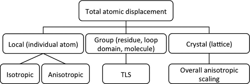
Hierarchy of contributions to atomic displacement parameters and possible ways to model these contributions (bottom row).

Each of these contributions can be described with different accuracy and using different models.

The common displacement of the crystal as a whole (lattice vibrations) (12, 14, 15) contributes equally to all atoms, and therefore it is possible to account for this effect directly while performing overall anisotropic scaling of the model with respect to the diffraction data.

Local atomic vibration can be described using an isotropic model that uses only one parameter per atom. A more detailed and accurate anisotropic parameterization uses six parameters but requires more experimental observations (higher resolution data sets) to be justified.

Similarly to local vibrations, different models can be used to describe group atomic displacement. For example, one can consider a special case of rigid-body motion that occurs around a fixed axis (10, 16). An example of such motion could be an oscillation of a flexible amino-acid side chain around C_α−C_β bond vector. When a rigid group oscillates, the term ‘libration’ is used instead of ‘rotation’ or ‘oscillation’ as it has been introduced in crystallography by Cruickshank (17). Such a libration can be described by a single parameter if the vibration law is known, e.g. for a harmonic one assuming small atomic displacements. More generally, any displacement of a rigid body may be considered as a superposition of a rotation around a given axis and a translation (see, for example (18)). Eventually, these two motions may be correlated. Nowadays the Translation-Libration-Screw-rotation (TLS) model of a rigid-body harmonic displacement (19) is the mostly widely used while other alternatives to modeling harmonic rigid-group displacement and refinement of corresponding parameters have been suggested previously (see for example (20, 21)). Here T, L and S are the model parameters that describe translation, libration and their correlation (screw-rotation), respectively. It has been demonstrated that the TLS model may provide reasonable results even for larger-scale vibrations (see for example (21)).

The aims, scope and results of this review include:

• comprehensive derivation of TLS equations from basic principles, incrementally going from simple special cases to more general ones;

• detailed analysis of TLS equations both for simple and general cases;

• discussion of some practical aspects relevant to TLS modeling.

We address these points, in spite of a very large amount of literature devoted to the TLS modeling (for example 3, 5, 13, 16, 19, 22–30 and references therein), because it is difficult to find corresponding derivations and formulae at a basic mathematical level permitting crystallographers with a non-mathematical background to understand and easily reproduce them. Apart from differences in notation and a few minor typographical errors found in the publications mentioned above, our resulting formulae are no different from those in the previous publications. However, such a comprehensive derivation allows a better understanding of the phenomenon and a better parameterization of the problem using parameters that have clear physical meaning and predictable range of values that they may accept (Section 5.6). The latter is particularly important for numerical protocols that are used to derive TLS matrices from experimental crystallographic data (TLS refinement). Moreover, such detailed analyses are not only important from a didactic viewpoint but also have clear applications in practice. In particular,

• we describe a step-by-step protocol for analysis of TLS matrices in terms of corresponding rigid-body motions of molecules or domains (Section 8.3); ready to program formulas and calculation schemes are provided;

• we consider a special case of TLS modeling to describe rigid-body libration around a fixed axis (Section 7); an illustration of such motion is a libration of an amino-acid residue side chain around corresponding bond; we believe that it is a better alternative to a traditional grouped ADP refinement and allows for modeling local anisotropy at a residue level of detail at medium to low resolution (Section 10) while no macromolecular structure refinement programs account for this type of motion at present;

• we propose a method to analyze TLS matrices in terms of ensemble of atomic models where each individual ensemble model is consistent with the TLS representation of concerted motion (Section 11).

Modeling atomic displacements is a complex subject. For example, TLS modeling requires identification of the rigid groups. Describing total atomic displacement requires not only accounting for TLS but also modeling other contributions (Figure 1). Refining various contributions to ADPs against experimental diffraction data is yet another topic. These problems are important but can be treated separately from each other. Here we focus on TLS modeling only and we refer only to the publications that we find most important or relevant on the subject. Some additional references that are relevant but not specifically discussed here are given in a complementary list at the end of the review.

There are a relatively large number of conventions and notations used in connection with ADPs (see (31) for a comprehensive review). In what follows we consistently use U assuming that the appropriate convention is used based on the context. We use capital letters for matrices, bold letters for vectors and italic for scalar parameters.

2. Description of motion

2.1. Atomic displacement parameter (ADP)

A crystallographic atomic model represents averaged positions r_n of atoms as well as the uncertainties in these positions. These uncertainties result in blurring of atomic peaks in the Fourier maps and they are described by atomic displacement parameters, ADP, in either isotropic or anisotropic form. To simplify the analysis we suppose that all unit cells of the crystal have exactly the same structure and all uncertainties in atomic positions arise from harmonic atomic motion only. Nowhere, except for Section 9, will we discuss diffraction from atoms. Rather, all procedures are purely geometric and for these reasons we consider ‘atoms’ as ‘point scatterers’ or simply as ‘geometric points’.

More formally, we suppose that there is a Cartesian coordinate system with the origin O and the three orthonormal basis vectors i, j,k (the vectors are orthogonal to each other and are of a unit length). A position of an atom n at a moment t is defined by the coordinates (x_n, y_n, z_n) of its averaged r_n position in this coordinate system and by the coordinates (q_nx (t),q_ny (t),q_nz (t)) of an instantaneous deviation q_n (t) from r_n. The electron density in each point r_n + q_n is proportional to the probability p_n (q_n) of finding the atom at q_n. This probability distribution, p_n(q_n), is positive and can be represented in Gaussian form around its peak (i.e. the most frequent position) and developed up to quadratic terms

$$p_n(\mathbf{q})\approx ={\kappa }_n·\text{exp}({\alpha }_{nxx}{q}_x^2+{\alpha }_{nyy}{q}_y^2+{\alpha }_{nzz}{q}_z^2+2{\alpha }_{nxy}{q}_x{q}_y+2{\alpha }_{nxz}{q}_x{q}_z+2{\alpha }_{nyz}{q}_y{q}_z)$$ (2.1)

Non-harmonic approximations are discussed for example in (2, 4, 5) and references therein.

Expression (2.1) can be put into a standard form using the matrix U_n defined as (see for example (32) and references therein)

$$U_n=\langle {\mathbf{q}}_n{\mathbf{q}}_n^{\tau }\rangle =\langle \left(\begin{array}{c}{q}_{nx}\hfill \\ q_{ny}\hfill \\ q_{nz}\hfill \end{array}\right)(\begin{array}{ccc}{q}_{nx}\hfill & q_{ny}\hfill & q_{nz}\hfill \end{array})\rangle =\left(\begin{array}{ccc}\hfill \langle q_{nx}^2\rangle \hfill & \hfill \langle q_{nx}{q}_{ny}\rangle \hfill & \hfill \langle q_{nx}{q}_{nz}\rangle \hfill \\ \hfill \langle q_{nx}{q}_{ny}\rangle \hfill & \hfill \langle q_{ny}^2\rangle \hfill & \hfill \langle q_{ny}{q}_{nz}\rangle \hfill \\ \hfill \langle q_{nx}{q}_{nz}\rangle \hfill & \hfill \langle q_{ny}{q}_{nz}\rangle \hfill & \hfill \langle q_{nz}^2\rangle \hfill \end{array}\right)$$ (2.2)

In (2.2) the symbol 〈〉 means the time average and index n in U_n means that each atom is related to its matrix of displacements. Here, and in what follows, the vector of instantaneous deviation q is represented by a column vector of its coordinates $\left(\begin{array}{c}{q}_x\hfill \\ q_y\hfill \\ q_z\hfill \end{array}\right)$ and τ signifies transposition, $(q_x,q_y,q_z)={\left(\begin{array}{c}{q}_x\hfill \\ q_y\hfill \\ q_z\hfill \end{array}\right)}^{\tau }$. The matrix (2.2) is positive definite. With (2.2) expression (2.1) becomes

$${(2\pi )}^{-3/2}{(\text{det}{U}_n)}^{-1/2}\text{exp}(-\frac{1}{2}{\mathbf{q}}^{\tau }{U}_n^{-1}\mathbf{q})$$ (2.3)

(see for example (4)), where U⁻¹ is the matrix inverse of U.

If a group of atoms moves together oscillating as a rigid body then the displacements q_n of these atoms are not independent but are expressed through some common parameters, and the corresponding U_n also can be expressed through several common parameters. A description of an atomic group as a rigid body is only an approximation; this problem and ways to take the next-level of detail into account have been discussed for example by (24, 33–38) and others.

It is worth noting that a physical phenomenon − the probability of atomic displacement q_n in the crystal − is invariant with respect to the mathematical description used to describe it. This means that if we change the coordinate system, the coordinates of q_n change, so the matrix U_n should change accordingly (Appendix A).

2.2. Rotation axes and their parameterization

To define a displacement of a rigid body with respect to its original position, one needs to know a translation vector, a rotation axis and a rotation angle. An axis may be characterized by a unit vector l = (l_x, l_y, l_z) along it and by a point w = (w_x, w_y, w_z) on the axis.

In order to define a position of the rotation axis parallel, for example, to the coordinate axis k (Figure 2a), two parameters are sufficient. For example these may be Cartesian coordinates of the point w = (w_x,w_y,0) at which this axis crosses the plane Oij. Alternatively, these may be polar coordinates R and α of this point. Note that, by construction, Ow is normal to k and therefore w is closest to the origin O among all points on the axis.

Figure 2.

Schematic illustration of the definition of a rotation axis l. (a) Axis parallel to k; its position is defined by 2 parameters, either by w_x and w_y, or by R and α. (b) Axis in an arbitrary orientation crossing the origin; its orientation is defined by 2 angles. (c) Axis in a general position; n is the vector parallel to l and crossing the origin; the plane normal to n and l is in grey. Similar to (b), two parameters are sufficient to define the orientation of n and l; to define the position of l two more parameters are required as in (a); they are coordinates of the intersection w of l with the grey plane. (d) Normalized Ow and l are the rotated i and k; p is the distance |Ow|.

For an arbitrary axis l that passes through the origin O (Figure 2b) two parameters are sufficient to define its direction. For example these may be two polar angles: the angle ψ between l and the k axis and the angle φ between i and the projection of l onto the plane Oij.

To fully define an axis in an arbitrary position and not crossing the origin O (Figure 2c), two parameters are required for its orientation, for example ψ and φ as above, and two more parameters for its position (l unambiguously defines the plane normal to it and containing the origin O; in this plane the two coordinates, Cartesian or polar, of the point w in which l crosses the plane define its position). Obviously other points w may be chosen as discussed later.

Alternatively, the sufficiency of 4 parameters can be understood as following. Let w be a point on the rotation axis l such that the vectors l and Ow are orthogonal; in other words w is in the plane normal to l and crossing the origin (Figure 2d). Then three Euler angles are sufficient to describe the orientation of Ow and l (for example a rotation of the basis vectors so that rotated i coincides with w and rotated k coincides with l) and the fourth parameter is the shift p of the l axis along the direction Ow.

2.3. Rotation: linear approximation

When considering a libration of a body around a given axis, a displacement of each point may be expanded as a power series in the rotation angle δ. Eventually, high-order series may be considered; see for example, (2, 3, 5) and references therein. Tickle & Moss (28) noted that “The harmonic model is applicable only if the motion is purely translational, but provided the libration amplitudes are not too large it is a good approximation”. Cruickshank (39) gave a value of 8° (0.14 radians) for the oscillation amplitude as a limit of this approximation.

In particular, working with small libration amplitudes means that a displacement towards the rotation axis is of the next order of magnitude compared to the displacement in the direction of the circle’s tangent. For example, when the body is rotated around the coordinate axis k by an angle δ the point r with the coordinates (1,0,0) moves to the coordinates (cosδ, sinδ, 0). Replacing the exact displacement (cosδ-1, sinδ, 0) by its linear approximation v we neglect all terms starting from δ² in the Taylor series for cosine and sine, and the approximate coordinates of the shift are

$$(\text{cos}\delta ,\text{sin}\delta ,0)-(1,0,0)\approx (0,\delta ,0)=\mathbf{v}$$ (2.4)

More generally, for small angles δ any point positioned at the distance R = 1 from the rotation axis is displaced by a distance d_z ≈ Rδ = δ (in radians). In these notes we use the parameter d_z (or d for rotation around an arbitrary axis) instead of δ to define the rotation amplitude.

Similarly (still within a linear approximation) each point in general position r_n = (x_n,y_n,z_n) is shifted in the direction normal to the rotation axis and normal to the vector r_n itself (Figure 3). In this example both points A=(x_n,0,0) and B=(x_n,0,z_n) are shifted by the vector (0, x_nd_z, 0), and the point C=(0,y_n,0) is shifted by (−y_nd_z, 0, 0). A general-position point r_n = (x_n,y_n,z_n) is shifted by

$${\mathbf{q}}_n\approx {\mathbf{v}}_n=(-y_n{d}_z,x_n{d}_z,0)=d_z[\mathbf{k}\times {\mathbf{r}}_n]$$ (2.5)

where × is a cross product.

Figure 3.

(a) Schematic illustration of the instantaneous displacement v (red vectors) of a point r (blue vectors) for a libration around the axis k. Each displacement vector is in the plane normal to k and also normal to the corresponding vector r. (b) Schematic illustration of a point r_n librating around the axis k. The mean (apparent) position of the point (dashed arrow) is in the middle of the circular segment OAB and is closer to the origin than the point itself.

For a rotation around an arbitrary axis l crossing the origin, a linear approximation v_n to the displacement q_n of a point r_n may be expressed similarly as

$${\mathbf{v}}_n=d[\mathit{l}\times {\mathbf{r}}_n]$$ (2.6)

The latter is often represented in an equivalent form

$${\mathbf{v}}_n=d{A}_n\mathit{l}$$ (2.7)

with the matrix

$$A_n=\left(\begin{array}{ccc}\hfill 0\hfill & \hfill z_n\hfill & \hfill -y_n\hfill \\ \hfill -z_n\hfill & \hfill 0\hfill & \hfill x_n\hfill \\ \hfill y_n\hfill & \hfill -x_n\hfill & \hfill 0\hfill \end{array}\right)$$ (2.8)

using Cartesian coordinates (x_n, y_n, z_n) of the point r_n in the coordinate system defined above (Section 2.1). If l passes through a point w = (w_x, w_y, w_z) and not through the origin O (see for example Section 2.2), vector v_n becomes

$${\mathbf{v}}_n=d[\mathit{l}\times ({\mathbf{r}}_n-\mathbf{w})]=d[\mathit{l}\times {\mathbf{r}}_n]-d[\mathit{l}\times \mathbf{w}]=d{A}_n\mathit{l}-d\mathit{l}\times \mathbf{w}$$ (2.9)

Here l × w is a constant vector, the same for all points of the oscillating rigid body; in contrast dA_nl is point-dependent as A_n is.

One can note that (2.9) presents a rotation around an axis in a general position as a rotation around an axis at the origin followed by a translation −dl × w common for all points and normal to the rotation axis. Conversely, a rotation around an axis at the origin (or at any other point) followed by a translation normal to it can be always represented as a pure rotation by the same angle as illustrated in Figure 4. The position of this rotation axis is unique. Figure 4 was inspired by Figure 2 in the TLSView Manual (40).

Figure 4.

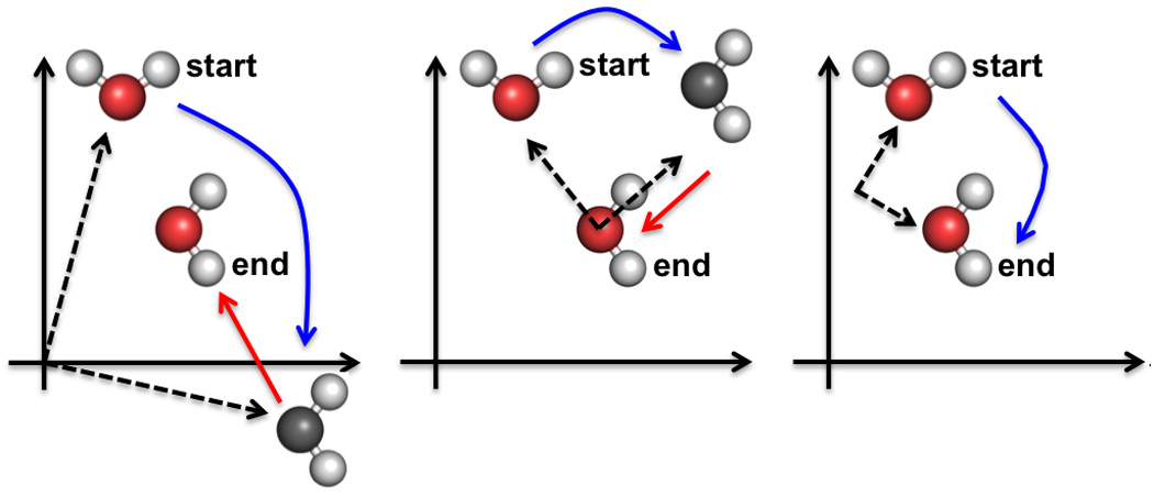
Three examples of possible combinations of a rotation (blue arrow) followed by a translation (red arrow) corresponding to the same transformation. The dashed lines show the vectors from the rotation axis, always perpendicular to the plane of the page, to the object. Left image: the axis crosses the origin. Middle image: the axis passes through the final position of the object; corresponding translation is smaller than in the left image. Right image: the same transformation performed as a pure rotation.

2.4. Choice of the point on the axis

Obviously, the shift (2.9) is independent of the choice of the point on the rotation axis l. If we substitute a point w by another point $\mathbf{w}\prime =(w_x^{\prime },w_y^{\prime },w_z^{\prime })$ on the same axis, this gives:

$${\mathbf{v}}_n^{\prime }=d[\mathit{l}\times ({\mathbf{r}}_n-\mathbf{w}\prime )]=d[\mathit{l}\times ({\mathbf{r}}_n-\mathbf{w}+\mathbf{w}-\mathbf{w}\prime )]==d[\mathit{l}\times ({\mathbf{r}}_n-\mathbf{w})]+d[\mathit{l}\times (\mathbf{w}-\mathbf{w}\prime )]=d[\mathit{l}\times ({\mathbf{r}}_n-\mathbf{w})]={\mathbf{v}}_n$$ (2.10)

since w − w′ is collinear with l.

2.5. Non-linear effects

When developing the libration-based shift (2.4)–(2.5) into the Taylor series on the rotation angle the (omitted) second-order term describes the displacement toward the rotation axis. This term is responsible for two effects (helpful illustrations of both can be found in (41, 42)). The first one is the curvature of electron density for individual atoms that appears as “banana-shaped contours” (27); some authors use the term “boomerang shape”. To the best of our knowledge such effects have not been reported in practical macromolecular studies.

The second effect is a shrinking of an apparent bond length (Figure 3b), the distance between the centers of two covalently linked atoms as we see them at the electron density maps of a high enough resolution, in comparison with the actual bond length. This problem was discussed in (16, 19, 36, 39, 43–46). Similarly, Scheringer (47) and Haestier et al. (48) discuss a modification of apparent bond angles. Cruickshank (39) and Haneef et al. (49) estimated the bond-length correction as 0.010–0.015 Å. According to Howlin et al. (27) these values may range up to 0.06 Å. Interestingly, Burns et al. (50) wrote that “… it has become fairly common practice at the end of a molecular crystal structure determination to analyze the anisotropic temperature parameters on the assumption that the molecule is rigid. Often the purpose is no more than the correction of bond lengths…”. Such examples can be found in (41, 42, 51–55).

We stress that this effect does not influence the atomic positions but, hypothetically, the target restraint values for bond lengths and angles should be libration-corrected thus becoming a function of the atomic displacement parameters.

In these notes we stay within a linear approximation (2.5–2.9).

3. Special case 1: rigid body translation

Translation is a special case of rigid body motion. For such a displacement all points of the body are shifted by the same vector q_n = u. For this particular motion we introduce a special notation for the matrix U_n (see formula 2.2), which is the same for all points of the group:

$$U_n=T=\left(\begin{array}{ccc}\hfill \langle u_x^2\rangle \hfill & \hfill \langle u_x{u}_y\rangle \hfill & \hfill \langle u_x{u}_z\rangle \hfill \\ \hfill \langle u_x{u}_y\rangle \hfill & \hfill \langle u_y^2\rangle \hfill & \hfill \langle u_y{u}_z\rangle \hfill \\ \hfill \langle u_x{u}_z\rangle \hfill & \hfill \langle u_y{u}_z\rangle \hfill & \hfill \langle u_z^2\rangle \hfill \end{array}\right)$$ (3.1)

By definition, T is symmetric and therefore is defined by 6 elements, 3 at the diagonal and 3 off-diagonal.

Also by definition T is non-negative definite, therefore it has three non-negative eigenvalues corresponding to three mutually orthogonal eigenvectors. In the basis composed of these normalized eigenvectors i_t, j_t, k_t, matrix T becomes

$$T_t=\left(\begin{array}{ccc}\hfill \langle t_x^2\rangle \hfill & \hfill 0\hfill & \hfill 0\hfill \\ \hfill 0\hfill & \hfill \langle t_y^2\rangle \hfill & \hfill 0\hfill \\ \hfill 0\hfill & \hfill 0\hfill & \hfill \langle t_z^2\rangle \hfill \end{array}\right)$$ (3.2)

with the eigenvalues at the diagonal. They are variances of the displacement along these three new axes. Zero off-diagonal elements mean that these displacements are uncorrelated with each other and that they can be used as three independent parameters describing the amplitudes of motion along these axes. Note that for an isotropic translational displacement the diagonal elements are all the same, $\langle t_x^2\rangle =\langle t_y^2\rangle =\langle t_z^2\rangle$, and therefore the matrix T is diagonal in any basis.

Since both the basis (i, j,k) and the basis (i_t, j_t, k_t) are orthonormal, the transformation between them may be only a rotation. The corresponding transformation matrix R_t (see Appendix A) can be defined by three rotation angles (56). Together with $\langle t_x^2\rangle ,\langle t_y^2\rangle ,\langle t_z^2\rangle$ this makes the total number of parameters equal to six.

Coordinates (t_x, t_y, t_z) of a shift u in the basis (i_t,j_t,k_t) are related to the coordinates (u_x, u_y, u_z) in the basis (i, j,k) by

$$\left(\begin{array}{c}\hfill u_x\hfill \\ \hfill u_y\hfill \\ \hfill u_z\hfill \end{array}\right)=R_t\left(\begin{array}{c}\hfill t_x\hfill \\ \hfill t_y\hfill \\ \hfill t_z\hfill \end{array}\right)$$ (3.3)

(Appendix A) and the matrix T in the initial basis is

$$T=R_t{T}_t{R}_t^{\tau }$$ (3.4)

4. Special case 2: rotation axis parallel to k

4.1. Rotation around k axis

Now we consider a pure rotation of a rigid body with no translation component. For simplicity, we start from a rotation by a small angle δ around the axis k. As shown in section 2.3, if d_z is a random value for a shift of a point at a distance equal to 1 from k, its probability distribution defines a corresponding shift q_n ≈ v_n = (−y_nd_z, x_nd_z, 0) of a point r_n = (x_n, y_n, z_n)giving its matrix U_n (2.2) as

$$U_n=\left(\begin{array}{ccc}\hfill \langle q_{nx}^2\rangle \hfill & \hfill \langle q_{nx}{q}_{ny}\rangle \hfill & \hfill \langle q_{nx}{q}_{nz}\rangle \hfill \\ \hfill \langle q_{nx}{q}_{ny}\rangle \hfill & \hfill \langle q_{ny}^2\rangle \hfill & \hfill \langle q_{ny}{q}_{nz}\rangle \hfill \\ \hfill \langle q_{nx}{q}_{nz}\rangle \hfill & \hfill \langle q_{ny}{q}_{nz}\rangle \hfill & \hfill \langle q_{nz}^2\rangle \hfill \end{array}\right)=\left(\begin{array}{ccc}\hfill y_n^2\langle d_z^2\rangle \hfill & \hfill -x_n{y}_n\langle d_z^2\rangle \hfill & \hfill 0\hfill \\ \hfill -x_n{y}_n\langle d_z^2\rangle \hfill & \hfill x_n^2\langle d_z^2\rangle \hfill & \hfill 0\hfill \\ \hfill 0\hfill & \hfill 0\hfill & \hfill 0\hfill \end{array}\right)==\langle d_z^2\rangle \left(\begin{array}{ccc}\hfill y_n^2\hfill & \hfill -x_n{y}_n\hfill & \hfill 0\hfill \\ \hfill -x_n{y}_n\hfill & \hfill x_n^2\hfill & \hfill 0\hfill \\ \hfill 0\hfill & \hfill 0\hfill & \hfill 0\hfill \end{array}\right)$$ (4.1)

This can be rewritten using matrix A_n (2.8)

$$U_n=\langle {\mathbf{q}}_n{\mathbf{q}}_n^{\tau }\rangle =\langle (d_z{A}_n\mathbf{k}){(d_z{A}_n\mathbf{k})}^{\tau }\rangle =\langle d_z^2{A}_n\mathbf{k}{\mathbf{k}}^{\tau }{A}_n^{\tau }\rangle =\langle d_z^2\rangle A_n\left(\begin{array}{ccc}\hfill 0\hfill & \hfill 0\hfill & \hfill 0\hfill \\ \hfill 0\hfill & \hfill 0\hfill & \hfill 0\hfill \\ \hfill 0\hfill & \hfill 0\hfill & \hfill 1\hfill \end{array}\right)A_n^{\tau }$$ (4.2)

4.2. Rotation around an axis parallel to k

When the rotation axis is parallel to k and passes through a point ${\mathbf{w}}^{\mathrm{k}}=(w_x^k,w_y^k,0)$ different from the origin, the corresponding shift (section 2.3) is

$${\mathbf{q}}_n\approx {\mathbf{v}}_n=d_z{A}_n\mathbf{k}-d_z\mathbf{k}\times \mathbf{w}=d_z{A}_n\mathbf{k}-d_z{W}_k\mathbf{k}=d_z{A}_n\mathbf{k}+d_z{W}_k^{\tau }\mathbf{k}$$ (4.3)

with

$$W_k=\left(\begin{array}{ccc}\hfill 0\hfill & \hfill 0\hfill & \hfill -w_y^k\hfill \\ \hfill 0\hfill & \hfill 0\hfill & \hfill w_x^k\hfill \\ \hfill w_y^k\hfill & \hfill -w_x^k\hfill & \hfill 0\hfill \end{array}\right)$$ (4.4)

Here matrix W_k is introduced similarly to matrix A_n in (2.6)–(2.7), section 2.3. Similarly to (4.2), expression (4.3) leads to

$$U_n==\langle d^2\rangle W_k^{\tau }(\mathbf{k}{\mathbf{k}}^{\tau })W_k+\langle d^2\rangle A_n(\mathbf{k}{\mathbf{k}}^{\tau })A_n^{\tau }+\langle d^2\rangle A_n(\mathbf{k}{\mathbf{k}}^{\tau })W_k+\langle d^2\rangle W_k^{\tau }(\mathbf{k}{\mathbf{k}}^{\tau })A_n^{\tau }$$ (4.5)

Here

$$\mathbf{k}{\mathbf{k}}^{\tau }=\left(\begin{array}{ccc}\hfill 0\hfill & \hfill 0\hfill & \hfill 0\hfill \\ \hfill 0\hfill & \hfill 0\hfill & \hfill 0\hfill \\ \hfill 0\hfill & \hfill 0\hfill & \hfill 1\hfill \end{array}\right)$$ (4.6)

and

$$\mathbf{k}{\mathbf{k}}^{\tau }{W}_k=\left(\begin{array}{ccc}\hfill 0\hfill & \hfill 0\hfill & \hfill 0\hfill \\ \hfill 0\hfill & \hfill 0\hfill & \hfill 0\hfill \\ \hfill w_y^k\hfill & \hfill -w_x^k\hfill & \hfill 0\hfill \end{array}\right),W_k^{\tau }\mathbf{k}{\mathbf{k}}^{\tau }=\left(\begin{array}{ccc}\hfill 0\hfill & \hfill 0\hfill & \hfill w_y^k\hfill \\ \hfill 0\hfill & \hfill 0\hfill & \hfill -w_x^k\hfill \\ \hfill 0\hfill & \hfill 0\hfill & \hfill 0\hfill \end{array}\right)$$ (4.7)

$$W_k^{\tau }\mathbf{k}{\mathbf{k}}^{\tau }{W}_k=\left(\begin{array}{ccc}\hfill {(w_y^k)}^2\hfill & \hfill -w_x^k{w}_y^k\hfill & \hfill 0\hfill \\ \hfill -w_x^k{w}_y^k\hfill & \hfill {(w_x^k)}^2\hfill & \hfill 0\hfill \\ \hfill 0\hfill & \hfill 0\hfill & \hfill 0\hfill \end{array}\right)$$ (4.8)

The first term in (4.5) is independent of the point and corresponds to an apparent translation even when there was no translation in the initial description of the motion (see section 2.3 for similar examples).

5. Special case 3: rotation around k combined with translation

5.1. Examples

Let's now consider that in addition to the rotation around k (Section 4.1) the body is undergoing a translation as described in Section 3, the total displacement of each point is the superposition of these two kinds of displacements. We start from some simple examples in order to illustrate the possible effects.

Let’s also suppose first that the random translational displacement is isotropic. When this is a single source of displacement, the position of the point will be spherically distributed around its central position r_n = (x_n, y_n, z_n) as shown in Figure 5a. This random distribution of the point’s position is illustrated by ‘electron clouds’ where more frequent positions have a darker color.

Figure 5.

Libration around the axis k and a random translation parallel to the rotation axis. (a) For a random isotropic translational displacement, the atomic position is spherically distributed around the central position A; more frequent positions are shown as darker. (b) In the presence of an additional libration, the spherical electron clouds are distributed along the arc (red arrow) or, in a linear approximation, along a line in the rotation plane and normal to OA. (c,d) When the displacement u (due to translation) along k is correlated with the rotational displacement v, the line along which the clouds are distributed (blue arrow) is no longer in the rotation plane, and its slope depends on the relation between the rotation and translation shifts (parameter s_z in text). The total displacement becomes a screw rotation. See Section 5.1 for more detail.

Let the same point have another source of displacement, a libration around a given axis, say for simplicity axis k. Now the point moves along an arc in the plane normal to the axis (red line in Figure 5b). In a linear approximation this arc can be considered to be a straight line that connects centers of blue spheres (− y_nd_z,x_nd_z,0).

Now let these two sources of displacement coexist. In the simplest case translation and libration are uncorrelated. This means that for any position generated by a libration an additional spherically distributed displacement due to translational movement can be added. In total, this generates the point positions distributed around the arc (Figure 5b).

Correlation of libration and translation displacements means that the individual displacements caused by these two sources are not independent of each other. Let us for the moment switch from a probabilistic to a deterministic model with a single translational component that is along the rotation axis. For example, the displacement along the axis may be proportional to the displacement due to rotation so that they are defined through the same random parameter d_z: (0,0,s_zd_z) and (− y_nd_z,x_nd_z,0), respectively; here s_z is some scale factor between them. The total displacements (− y_nd_z, x_nd_z, s_zd_z) follow a line crossing the rotation plane. It is easy to show that this line is in the plane normal to the vector r_n (blue line in the grey plane in Figures 5c,d). For larger rotational amplitude the displacement is no longer approximately linear and instead follows a helix. This defines a new type of motion, a screw rotation. Depending on the sign of s_z, the helix may be right- or left-handed. If the displacements are again random, the set of displacements form spherical clouds, similarly to Figures 5a,b, centered now on this helix (Figures 5c,d).

Correlated libration and displacement in the direction normal to the rotation axis leads to a totally different effect. Figure 6a represents the displacements (− y_nd_z,x_nd_z,0) of a point in the rotation plane due to libration around k (red arrows). A random isotropic translational displacement is illustrated by a grey ‘cloud’, as in Figure 5a. A superposition of rotation and translation moves the cloud along the circle, or, in linear approximation, along a line normal to the radius; the same as in Figure 5b. Figure 6b shows schematically the displacements in a presence of a dominant translation component in the direction Ox (black arrows) instead of libration; note a similarity of positions for points A and C. When both libration and translational displacement in the direction Ox occur simultaneously and are highly correlated they may be expressed through the same libration parameter d_z. As for the previous example, the corresponding shifts are (− y_nd_z,x_nd_z,0) and (s_xd_z,0,0) with some scale factor s_x, and the total instantaneous displacement (blue arrow in Figures 6d,f) of a point is equal to (s_xd_z − y_nd_z,x_nd_z,0). This means that the point O = (0,0,0), which belongs to the rotation axis, now moves from its position, and also there are new immobile points, those with the coordinates (0,s_x,z). In Figures 6d and 6f the point A is such an immobile point; for smaller s_x the apparent axis will be closer to O. The presence of immobile points means that such a movement is a rotation with the same random parameter d_z but around an apparent axis parallel to k and shifted from the origin by the vector (0,s_x,0). In the presence of random isotropic translation motion, each point’s position is replaced by a cloud around it.

Figure 6.

Correlation of a libration around an axis k and a translation in the normal direction, i; the projection normal to k is shown. (a) For a pure libration around O, in a linear approximation all points (A,B,C,D in this case) move perpendicularly to the corresponding radius, shown as red arrows. The presence of a random isotropic translation displacement is illustrated by spherical clouds around each position. (b) For a pure translation in the direction i, displacements of all points are the same, black arrows. Overall clouds for A and C are the same as in (a). (c) An instantaneous displacement due to counter-clockwise libration (red arrow). Centers of electron clouds shift from their grey positions toward the blue ones. d) A translation component (black arrow) added to libration (c) and highly correlated with it, e.g. it is always equal to the displacement of the point C due to libration. The resulted displacements are shown by blue arrows. Point A is immobile. (e,f) are similar to (c,d) and show a clockwise instantaneous rotation around O and the corresponding translation. Movements in (d) and (f) are rotations around an apparent axis normal to the plane and crossing it in the point A. As for (a) and (b), the random isotropic translation is illustrated by a grey cloud for the initial position and by a blue cloud for a shifted position. See section 5.1 for more details.

Since each rigid-body motion is a combination of rotation and translation, and each translation can be decomposed along the instantaneous rotation axis and normal to it, the examples above cover all possible combinations. Sections below analyze these situations in a more formal and general way.

5.2. Screw axes along k

Let’s analyze a screw rotation around an axis k more formally. As discussed in the previous Section, the corresponding displacement of a point (x_n, y_n, z_n) is

$${\mathbf{q}}_n=(-y_n{d}_z,x_n{d}_z,s_z{d}_z)=d_z{A}_n\mathbf{k}+s_z{d}_z\mathbf{k}$$ (5.1)

The component s_zd_zk is the same for all points of the rigid body and it is a translation component of the group. Accordingly (2.2) the matrix U_n is

$$U_n=s_z^2\langle d_z^2\rangle (\mathbf{k}{\mathbf{k}}^{\tau })+A_n\langle d_z^2\rangle (\mathbf{k}{\mathbf{k}}^{\tau })A_n^{\tau }+A_n(s_z\langle d_z^2\rangle \mathbf{k}{\mathbf{k}}^{\tau })+(s_z\langle d_z^2\rangle \mathbf{k}{\mathbf{k}}^{\tau })A_n^{\tau }$$ (5.2)

One may note a similarity between (5.2) and (4.5). The first term in (5.2) is independent of the atomic coordinates and signifies the translation of the group. The second term is a quadratic function of atomic coordinates (through matrix A_n) and corresponds to the group rotation. Two last terms in (5.2) depend on atomic coordinates linearly and are due to the screw component. Following (19) we associate these terms with the matrices T, L and S that we define here as

$$T=\left(\begin{array}{ccc}\hfill 0\hfill & \hfill 0\hfill & \hfill 0\hfill \\ \hfill 0\hfill & \hfill 0\hfill & \hfill 0\hfill \\ \hfill 0\hfill & \hfill 0\hfill & \hfill s_z^2\langle d_z^2\rangle \hfill \end{array}\right)$$ (5.3)

$$L=\left(\begin{array}{ccc}\hfill 0\hfill & \hfill 0\hfill & \hfill 0\hfill \\ \hfill 0\hfill & \hfill 0\hfill & \hfill 0\hfill \\ \hfill 0\hfill & \hfill 0\hfill & \hfill \langle d_z^2\rangle \hfill \end{array}\right)$$ (5.4)

$$S=\left(\begin{array}{ccc}\hfill 0\hfill & \hfill 0\hfill & \hfill 0\hfill \\ \hfill 0\hfill & \hfill 0\hfill & \hfill 0\hfill \\ \hfill 0\hfill & \hfill 0\hfill & \hfill s_z\langle d_z^2\rangle \hfill \end{array}\right)$$ (5.5)

Using matrices T, L and S we can rewrite (5.2) as

$$U_n=T+A_{n}L{A}_n^{\tau }+A_{n}S+{(A_{n}S)}^{\tau }$$ (5.6)

5.3. TLS representation

Now let’s generalize the examples from Sections 5.1 and 5.2. We keep the same notation and use u for translational displacement (Section 3) and v_n for the displacement due to libration around axis k, always in a linear approximation (Section 2.3).

For an atom n with Cartesian coordinates (x_n, y_n, z_n) the total displacement vector

$${\mathbf{q}}_n=\mathbf{u}+{\mathbf{v}}_n=\mathbf{u}+d_z{A}_n\mathbf{k}$$ (5.7)

has the coordinates

$$\left(\begin{array}{c}\hfill q_{nx}\hfill \\ \hfill q_{ny}\hfill \\ \hfill q_{nz}\hfill \end{array}\right)=\left(\begin{array}{c}\hfill u_x\hfill \\ \hfill u_y\hfill \\ \hfill u_z\hfill \end{array}\right)+\left(\begin{array}{c}\hfill -y_n{d}_z\hfill \\ \hfill x_n{d}_z\hfill \\ \hfill 0\hfill \end{array}\right)=\left(\begin{array}{c}\hfill u_x-y_n{d}_z\hfill \\ \hfill u_y+x_n{d}_z\hfill \\ \hfill u_z\hfill \end{array}\right)$$ (5.8)

where d_z, as previously, defines the linear approximation (0,d_z,0) to the displacement of the point (1,0,0). Note that, as follows from Section 5.2, translation vector u may include the screw component and therefore it can be correlated with the rotation.

Components of the matrix U_n (2.2) in the same coordinate system (i, j, k):

$$U_{nxx}=\langle {(u_x-y_n{d}_z)}^2\rangle =\langle u_x^2+y_n^2{d}_z^2-2y_n{u}_x{d}_z\rangle =\langle u_x^2\rangle +y_n^2\langle d_z^2\rangle -2y_n\langle u_x{d}_z\rangle U_{nyy}=\langle {(u_y+x_n{d}_z)}^2\rangle =\langle u_y^2+x_n^2{d}_z^2+2x_n{u}_y{d}_z\rangle =\langle u_y^2\rangle +x_n^2\langle d_z^2\rangle +2x_n\langle u_y{d}_z\rangle U_{nzz}=\langle u_z^2\rangle U_{nyz}=U_{nzy}=\langle (u_y+x_n{d}_z)u_z\rangle =\langle u_y{u}_z+x_n{u}_z{d}_z\rangle =\langle u_y{u}_z\rangle +x_n\langle u_z{d}_z\rangle U_{nzx}=U_{nxz}=\langle (u_x-y_n{d}_z)u_z\rangle =\langle u_x{u}_z-y_n{u}_z{d}_z\rangle =\langle u_x{u}_z\rangle -y_n\langle u_z{d}_z\rangle U_{nxy}=U_{nyx}=\langle (u_x-y_n{d}_z)(u_y+x_n{d}_z)\rangle =\langle u_x{u}_y-y_n{u}_y{d}_z+x_n{u}_x{d}_z-x_n{y}_n{d}_z^2\rangle ==\langle u_x{u}_y\rangle -y_n\langle u_y{d}_z\rangle +x\langle u_x{d}_z\rangle -x_n{y}_n\langle d_z^2\rangle$$ (5.9)

Similarly to Section 5.2, we can use the form

$$U_n=T+A_{n}L{A}_n^{\tau }+A_{n}S+S^{\tau }{A}_n^{\tau }$$ (5.10)

similar to (5.6), where

$$T=U_T=\left(\begin{array}{ccc}\hfill \langle u_x^2\rangle \hfill & \hfill \langle u_x{u}_y\rangle \hfill & \hfill \langle u_x{u}_z\rangle \hfill \\ \hfill \langle u_x{u}_y\rangle \hfill & \hfill \langle u_y^2\rangle \hfill & \hfill \langle u_y{u}_z\rangle \hfill \\ \hfill \langle u_x{u}_z\rangle \hfill & \hfill \langle u_y{u}_z\rangle \hfill & \hfill \langle u_z^2\rangle \hfill \end{array}\right)$$ (5.11)

$$L=\left(\begin{array}{ccc}\hfill 0\hfill & \hfill 0\hfill & \hfill 0\hfill \\ \hfill 0\hfill & \hfill 0\hfill & \hfill 0\hfill \\ \hfill 0\hfill & \hfill 0\hfill & \hfill \langle d_z^2\rangle \hfill \end{array}\right)$$ (5.12)

$$S=\left(\begin{array}{ccc}\hfill 0\hfill & \hfill 0\hfill & \hfill 0\hfill \\ \hfill 0\hfill & \hfill 0\hfill & \hfill 0\hfill \\ \hfill \langle u_x{d}_z\rangle \hfill & \hfill \langle u_y{d}_z\rangle \hfill & \hfill \langle u_z{d}_z\rangle \hfill \end{array}\right)$$ (5.13)

and

$$A_n=\left(\begin{array}{ccc}\hfill 0\hfill & \hfill z_n\hfill & \hfill -y_n\hfill \\ \hfill -z_n\hfill & \hfill 0\hfill & \hfill x_n\hfill \\ \hfill y_n\hfill & \hfill -x_n\hfill & \hfill 0\hfill \end{array}\right)$$ (5.14)

In 5.10 through 5.14 matrices T, L, S are the same for all points of the rigid body while A_n is expressed through the coordinates of the point.

Expressions 5.11 through 5.13 show the 10 parameters common for the rigid group: 6, 1 and 3 parameters associated with T, L, S, respectively. Together with the matrices A_n, they fully define U_n for all atoms in the rigid group.

5.4. U_n and the choice of origin

5.4.1. Theory

Obviously, matrices U_n do not depend on the choice of the origin of the coordinate system while matrices A_n do. The relation (5.10) means that T, L, S also depend on the origin. We will demonstrate this dependency, which is important for further analysis.

In a new coordinate system with the origin shifted by vector p = (p_x, p_y, p_z)

$$\mathbf{O}\prime =\mathbf{O}+\mathbf{p}$$ (5.15)

the new coordinates are x_n − p_x, y_n − p_y,z_n − p_z defining the matrix

$$A_n^{\prime }=\left(\begin{array}{ccc}\hfill 0\hfill & \hfill z_n-p_z\hfill & \hfill -(y_n-p_y)\hfill \\ \hfill -(z_n-p_z)\hfill & \hfill 0\hfill & \hfill x_n-p_x\hfill \\ \hfill y_n-p_y\hfill & \hfill -(x_n-p_x)\hfill & \hfill 0\hfill \end{array}\right)==\left(\begin{array}{ccc}\hfill 0\hfill & \hfill z_n\hfill & \hfill -y_n\hfill \\ \hfill -z_n\hfill & \hfill 0\hfill & \hfill x\hfill \\ \hfill y_n\hfill & \hfill -x_n\hfill & \hfill 0\hfill \end{array}\right)-\left(\begin{array}{ccc}\hfill 0\hfill & \hfill p_z\hfill & \hfill -p_y\hfill \\ \hfill -p_z\hfill & \hfill 0\hfill & \hfill p_x\hfill \\ \hfill p_y\hfill & \hfill -p_x\hfill & \hfill 0\hfill \end{array}\right)=A_n-P$$ (5.16)

(for convenience of further analysis, we define the shift vector in the opposite way to (28)). Matrix P in (5.16) is the same for all points of the group. Accordingly to (5.10) matrix U_n becomes

$$U_n=T+(A_n^{\prime }+P)L{(A_n^{\prime }+P)}^{\tau }+(A_n^{\prime }+P)S+S^{\tau }{(A_n^{\prime }+P)}^{\tau }==T+(A_n^{\prime }L{A}_n^{\prime \tau }+A_n^{\prime }L{P}^{\tau }+PL{A}_n^{\prime \tau }+PL{P}^{\tau })+(A_n^{\prime }S+PS)+(S^{\tau }{A}_n^{\prime \tau }+S^{\tau }{P}^{\tau })==(T+PL{P}^{\tau }+PS+S^{\tau }{P}^{\tau })+A_n^{\prime }L{A}_n^{\prime \tau }+A_n^{\prime }(S+L{P}^{\tau })+(S^{\tau }+P{L}^{\tau })A_n^{\prime \tau }==T\prime +A_n^{\prime }L\prime A_n^{\prime \tau }+A_n^{\prime }S\prime +S^{\prime \tau }{A}_n^{\prime \tau }=U_n^{\prime }$$ (5.17)

(in the last equality we substituted $PL{A}_n^{\prime \tau }$ by PL^τ $A_n^{\prime \tau }$ using the symmetry L = L^τ). Comparison with (5.10) defines new matrices T′,L′,S′ as

$$T\prime =T+(PL{P}^{\tau }+PS+S^{\tau }{P}^{\tau })L\prime =LS\prime =S+L{P}^{\tau }-LP$$ (5.18)

since P is antisymmetric. It is important that the expressions (5.18) were obtained for the matrices T, L, S with no use of their specific form (5.11–5.13). This means that (5.18) can be applied also to T, L, S in a general case of motion.

A simple example illustrating (5.18) is represented below.

5.4.2. Example

Let’s suppose that a rigid group oscillates around the axis k. In this case the only non-zero matrix is L (5.6) while T and S are zero. For the point M = (0,0,0) its $A_n=\left(\begin{array}{ccc}\hfill 0\hfill & \hfill 0\hfill & \hfill 0\hfill \\ \hfill 0\hfill & \hfill 0\hfill & \hfill 0\hfill \\ \hfill 0\hfill & \hfill 0\hfill & \hfill 0\hfill \end{array}\right)$ giving zero matrix U_n (as the point is on the rotation axis). Now let’s choose another coordinate system shifting the origin by p = (1,0,0). The new coordinates of the point M are (−1,0,0), its new matrix $A_n^{\prime }=\left(\begin{array}{ccc}\hfill 0\hfill & \hfill 0\hfill & \hfill 0\hfill \\ \hfill 0\hfill & \hfill 0\hfill & \hfill -1\hfill \\ \hfill 0\hfill & \hfill 1\hfill & \hfill 0\hfill \end{array}\right)$, and matrix $P=\left(\begin{array}{ccc}\hfill 0\hfill & \hfill 0\hfill & \hfill 0\hfill \\ \hfill 0\hfill & \hfill 0\hfill & \hfill 1\hfill \\ \hfill 0\hfill & \hfill -1\hfill & \hfill 0\hfill \end{array}\right)$. New matrices are

$$S\prime =\left(\begin{array}{ccc}\hfill 0\hfill & \hfill 0\hfill & \hfill 0\hfill \\ \hfill 0\hfill & \hfill 0\hfill & \hfill 0\hfill \\ \hfill 0\hfill & \hfill 0\hfill & \hfill \langle d_z^2\rangle \hfill \end{array}\right)\left(\begin{array}{ccc}\hfill 0\hfill & \hfill 0\hfill & \hfill 0\hfill \\ \hfill 0\hfill & \hfill 0\hfill & \hfill -1\hfill \\ \hfill 0\hfill & \hfill 1\hfill & \hfill 0\hfill \end{array}\right)=\left(\begin{array}{ccc}\hfill 0\hfill & \hfill 0\hfill & \hfill 0\hfill \\ \hfill 0\hfill & \hfill 0\hfill & \hfill 0\hfill \\ \hfill 0\hfill & \hfill \langle d_z^2\rangle \hfill & \hfill 0\hfill \end{array}\right)A_n^{\prime }S\prime =\left(\begin{array}{ccc}\hfill 0\hfill & \hfill 0\hfill & \hfill 0\hfill \\ \hfill 0\hfill & \hfill 0\hfill & \hfill -1\hfill \\ \hfill 0\hfill & \hfill 1\hfill & \hfill 0\hfill \end{array}\right)\left(\begin{array}{ccc}\hfill 0\hfill & \hfill 0\hfill & \hfill 0\hfill \\ \hfill 0\hfill & \hfill 0\hfill & \hfill 0\hfill \\ \hfill 0\hfill & \hfill \langle d_z^2\rangle \hfill & \hfill 0\hfill \end{array}\right)=\left(\begin{array}{ccc}\hfill 0\hfill & \hfill 0\hfill & \hfill 0\hfill \\ \hfill 0\hfill & \hfill -\langle d_z^2\rangle \hfill & \hfill 0\hfill \\ \hfill 0\hfill & \hfill 0\hfill & \hfill 0\hfill \end{array}\right)T\prime =\left(\begin{array}{ccc}\hfill 0\hfill & \hfill 0\hfill & \hfill 0\hfill \\ \hfill 0\hfill & \hfill 0\hfill & \hfill 1\hfill \\ \hfill 0\hfill & \hfill -1\hfill & \hfill 0\hfill \end{array}\right)\left(\begin{array}{ccc}\hfill 0\hfill & \hfill 0\hfill & \hfill 0\hfill \\ \hfill 0\hfill & \hfill 0\hfill & \hfill 0\hfill \\ \hfill 0\hfill & \hfill 0\hfill & \hfill \langle d_z^2\rangle \hfill \end{array}\right)\left(\begin{array}{ccc}\hfill 0\hfill & \hfill 0\hfill & \hfill 0\hfill \\ \hfill 0\hfill & \hfill 0\hfill & \hfill -1\hfill \\ \hfill 0\hfill & \hfill 1\hfill & \hfill 0\hfill \end{array}\right)=\left(\begin{array}{ccc}\hfill 0\hfill & \hfill 0\hfill & \hfill 0\hfill \\ \hfill 0\hfill & \hfill \langle d_z^2\rangle \hfill & \hfill 0\hfill \\ \hfill 0\hfill & \hfill 0\hfill & \hfill 0\hfill \end{array}\right)A_n^{\prime }L\prime A_n^{\prime \tau }=\left(\begin{array}{ccc}\hfill 0\hfill & \hfill 0\hfill & \hfill 0\hfill \\ \hfill 0\hfill & \hfill 0\hfill & \hfill -1\hfill \\ \hfill 0\hfill & \hfill 1\hfill & \hfill 0\hfill \end{array}\right)\left(\begin{array}{ccc}\hfill 0\hfill & \hfill 0\hfill & \hfill 0\hfill \\ \hfill 0\hfill & \hfill 0\hfill & \hfill 0\hfill \\ \hfill 0\hfill & \hfill 0\hfill & \hfill \langle d_z^2\rangle \hfill \end{array}\right)\left(\begin{array}{ccc}\hfill 0\hfill & \hfill 0\hfill & \hfill 0\hfill \\ \hfill 0\hfill & \hfill 0\hfill & \hfill 1\hfill \\ \hfill 0\hfill & \hfill -1\hfill & \hfill 0\hfill \end{array}\right)=\left(\begin{array}{ccc}\hfill 0\hfill & \hfill 0\hfill & \hfill 0\hfill \\ \hfill 0\hfill & \hfill \langle d_z^2\rangle \hfill & \hfill 0\hfill \\ \hfill 0\hfill & \hfill 0\hfill & \hfill 0\hfill \end{array}\right)$$

The new matrix $U_n^{\prime }=T\prime +A_n^{\prime }L\prime A_n^{\prime \tau }+A_n^{\prime }S\prime +S^{\prime \tau }{A}_n^{\prime \tau }$ for the point M is a zero matrix as it should be.

5.5. Search for the apparent rotation axis

An example considered in Section 5.1 shows that a combination of a libration and a translation in the direction normal to the axis may be described by a single motion, a libration around an apparent axis. This simplifies the description of the motion. In this section we show the corresponding results for a rotation around k. Applying (5.18) with matrix P of a general form (5.16) to (5.11–5.13) gives

$$L{P}^{\tau }=\left(\begin{array}{ccc}\hfill 0\hfill & \hfill 0\hfill & \hfill 0\hfill \\ \hfill 0\hfill & \hfill 0\hfill & \hfill 0\hfill \\ \hfill -p_y\langle d_z^2\rangle \hfill & \hfill p_x\langle d_z^2\rangle \hfill & \hfill 0\hfill \end{array}\right)$$ (5.19)

$$S+L{P}^{\tau }=\left(\begin{array}{ccc}\hfill 0\hfill & \hfill 0\hfill & \hfill 0\hfill \\ \hfill 0\hfill & \hfill 0\hfill & \hfill 0\hfill \\ \hfill \langle u_x{d}_z\rangle -p_y\langle d_z^2\rangle \hfill & \hfill \langle u_y{d}_z\rangle +p_x\langle d_z^2\rangle \hfill & \hfill \langle u_z{d}_z\rangle \hfill \end{array}\right)$$ (5.20)

$$PL{P}^{\tau }=\left(\begin{array}{ccc}\hfill p_y^2\langle d_z^2\rangle \hfill & \hfill -p_x{p}_y\langle d_z^2\rangle \hfill & \hfill 0\hfill \\ \hfill -p_x{p}_y\langle d_z^2\rangle \hfill & \hfill p_x^2\langle d_z^2\rangle \hfill & \hfill 0\hfill \\ \hfill 0\hfill & \hfill 0\hfill & \hfill 0\hfill \end{array}\right)$$ (5.21)

$$PS=\left(\begin{array}{ccc}\hfill -p_y\langle u_x{d}_z\rangle \hfill & \hfill -p_y\langle u_y{d}_z\rangle \hfill & \hfill -p_y\langle u_z{d}_z\rangle \hfill \\ \hfill p_x\langle u_x{d}_z\rangle \hfill & \hfill p_x\langle u_y{d}_z\rangle \hfill & \hfill p_x\langle u_z{d}_z\rangle \hfill \\ \hfill 0\hfill & \hfill 0\hfill & \hfill 0\hfill \end{array}\right)$$ (5.22)

$$T+PL{P}^{\tau }+PS+S^{\tau }{P}^{\tau }==\left(\begin{array}{ccc}\hfill \langle u_x^2\rangle +p_y^2\langle d_z^2\rangle -2p_y\langle u_x{d}_z\rangle \hfill & \hfill \{\langle u_x{u}_y\rangle -p_x{p}_y\langle d_z^2\rangle ++p_x\langle u_x{d}_z\rangle -p_y\langle u_y{d}_z\rangle \}\hfill & \hfill \langle u_x{u}_z\rangle -p_y\langle u_z{d}_z\rangle \hfill \\ \hfill \{\langle u_x{u}_y\rangle -p_x{p}_y\langle d_z^2\rangle ++p_x\langle u_x{d}_z\rangle -p_y\langle u_y{d}_z\rangle \}\hfill & \hfill \langle u_y^2\rangle +p_x^2\langle d_z^2\rangle +2p_x\langle u_y{d}_z\rangle \hfill & \hfill \langle u_y{u}_z\rangle +p_x\langle u_z{d}_z\rangle \hfill \\ \hfill \langle u_x{u}_z\rangle -p_y\langle u_z{d}_z\rangle \hfill & \hfill \langle u_y{u}_z\rangle +p_x\langle u_z{d}_z\rangle \hfill & \hfill \langle u_z^2\rangle \hfill \end{array}\right)$$ (5.23)

Expression (5.20) shows the existence of a special origin

$$p_y=\frac{\langle u_x{d}_z\rangle }{\langle d_z^2\rangle },p_x=-\frac{\langle u_y{d}_z\rangle }{\langle d_z^2\rangle }.$$ (5.24)

that reduces the matrix S to

$$S\prime =S+L{H}^{\tau }=\left(\begin{array}{ccc}\hfill 0\hfill & \hfill 0\hfill & \hfill 0\hfill \\ \hfill 0\hfill & \hfill 0\hfill & \hfill 0\hfill \\ \hfill 0\hfill & \hfill 0\hfill & \hfill \langle u_z{d}_z\rangle \hfill \end{array}\right).$$ (5.25)

This means that with the new origin there is no correlation between rotation and translation displacements in the plane normal to the rotation axis (axis k in this example), i.e. that the apparent rotation axis crosses the new origin (see Section 5.1; compare also (5.24) with (4.4)). Logically, the result is independent of p_z which is an origin shift along the rotation axis.

With this choice of the origin, matrix T (5.23) becomes

$$T\prime =\left(\begin{array}{ccc}\hfill \langle u_x^2\rangle -\frac{{\langle u_x{d}_z\rangle }^2}{\langle d_z^2\rangle }\hfill & \hfill \langle u_x{u}_y\rangle -\frac{\langle u_x{d}_z\rangle \langle u_y{d}_z\rangle }{\langle d_z^2\rangle }\hfill & \hfill \langle u_x{u}_z\rangle -\frac{\langle u_x{d}_z\rangle \langle u_z{d}_z\rangle }{\langle d_z^2\rangle }\hfill \\ \hfill \langle u_x{u}_y\rangle -\frac{\langle u_x{d}_z\rangle \langle u_y{d}_z\rangle }{\langle d_z^2\rangle }\hfill & \hfill \langle u_y^2\rangle -\frac{{\langle u_y{d}_z\rangle }^2}{\langle d_z^2\rangle }\hfill & \hfill \langle u_y{u}_z\rangle -\frac{\langle u_y{d}_z\rangle \langle u_z{d}_z\rangle }{\langle d_z^2\rangle }\hfill \\ \hfill \langle u_x{u}_z\rangle -\frac{\langle u_x{d}_z\rangle \langle u_z{d}_z\rangle }{\langle d_z^2\rangle }\hfill & \hfill \langle u_y{u}_z\rangle -\frac{\langle u_y{d}_z\rangle \langle u_z{d}_z\rangle }{\langle d_z^2\rangle }\hfill & \hfill \langle u_z^2\rangle \hfill \end{array}\right)$$ (5.26)

Here all diagonal elements of (5.23) reach their minimum by p, as well as obviously the trace of the matrix, $tr\left(T\right)=T_{xx}+T_{yy}+T_{zz}\to \underset{p_x,p_y,p_z}{\text{min}}$ (19, 28, 57).

5.6. Parameters with a physical meaning

Similarly to Section 3, one may define the elements of T through its eigenvalues (uncorrelated translations) $\langle t_x^2\rangle ,\langle t_y^2\rangle ,\langle t_z^2\rangle$ and the rotation matrix R_t. One may also note that due to relation (3.3)

$$\left(\begin{array}{c}\hfill \langle u_x{d}_z\rangle \hfill \\ \hfill \langle u_y{d}_z\rangle \hfill \\ \hfill \langle u_z{d}_z\rangle \hfill \end{array}\right)=R_t\left(\begin{array}{c}\hfill \langle t_x{d}_z\rangle \hfill \\ \hfill \langle t_y{d}_z\rangle \hfill \\ \hfill \langle t_z{d}_z\rangle \hfill \end{array}\right)$$ (5.27)

where 〈t_xd_z〉, 〈t_yd_z〉, 〈t_zd_z〉 describe correlation of random displacements (t_x, t_y, t_z), uncorrelated with each other, with the displacement due to libration around the axis k, and the matrix R_t is the same as before.

Moreover, one may introduce the correlations

$$-1\le c_x=\frac{\langle t_x{d}_z\rangle }{\sqrt{\langle t_x^2\rangle }\sqrt{\langle d_z^2\rangle }}\le 1,-1\le c_y=\frac{\langle t_y{d}_z\rangle }{\sqrt{\langle t_y^2\rangle }\sqrt{\langle d_z^2\rangle }}\le 1,-1\le c_z=\frac{\langle t_z{d}_z\rangle }{\sqrt{\langle t_z^2\rangle }\sqrt{\langle d_z^2\rangle }}\le 1$$ (5.28)

as independent parameters instead of 〈u_xd_z〉, 〈u_yd_z〉, 〈u_zd_z〉, resulting in another set of ten parameters: $\langle t_x^2\rangle ,\langle t_y^2\rangle ,\langle t_z^2\rangle ,\langle d_z^2\rangle$, c_x, c_y, c_z, and three mutually orthogonal directions of uncorrelated translations described through R_t by three Euler angles. Such a choice has an advantage that all corresponding parameters have a clear physical meaning and predictable range of values.

6. Special case 4: three rotation axes parallel to ijk

6.1. Uncorrelated pure rotations

Now we will extend the analysis from Section 4.2. When a rotation axis is parallel to i or j instead of k, the resulting matrix has always the form (4.5) in which W_k and kk^τ (4.4 and 4.6) are replaced by

$$W_i=\left(\begin{array}{ccc}\hfill 0\hfill & \hfill w_z^i\hfill & \hfill -w_y^i\hfill \\ \hfill -w_z^i\hfill & \hfill 0\hfill & \hfill 0\hfill \\ \hfill w_y^i\hfill & \hfill 0\hfill & \hfill 0\hfill \end{array}\right)\text{and}\mathbf{i}{\mathbf{i}}^{\tau }=\left(\begin{array}{ccc}\hfill 1\hfill & \hfill 0\hfill & \hfill 0\hfill \\ \hfill 0\hfill & \hfill 0\hfill & \hfill 0\hfill \\ \hfill 0\hfill & \hfill 0\hfill & \hfill 0\hfill \end{array}\right)$$ (6.1)

for rotations around i or by

$$W_j=\left(\begin{array}{ccc}\hfill 0\hfill & \hfill w_z^j\hfill & \hfill 0\hfill \\ \hfill -w_z^j\hfill & \hfill 0\hfill & \hfill w_x^j\hfill \\ \hfill 0\hfill & \hfill -w_x^j\hfill & \hfill 0\hfill \end{array}\right)\text{and}\mathbf{j}{\mathbf{j}}^{\tau }=\left(\begin{array}{ccc}\hfill 0\hfill & \hfill 0\hfill & \hfill 0\hfill \\ \hfill 0\hfill & \hfill 1\hfill & \hfill 0\hfill \\ \hfill 0\hfill & \hfill 0\hfill & \hfill 0\hfill \end{array}\right)$$ (6.2)

for rotations around j, respectively.

When three rotations around the axes parallel to i, j and k with the corresponding amplitudes d_x, d_y, d_z are applied simultaneously (see Figure 2 in Schomaker & Trueblood (19) for an illustration) the resulting shift is the sum of the shifts caused by the respective rotations

$${\mathbf{q}}_n\approx {\mathbf{v}}_n=(d_x{A}_n\mathbf{i}+d_x{W}_i^{\tau }\mathbf{i})+(d_y{A}_n\mathbf{j}+d_y{W}_j^{\tau }\mathbf{j})+(d_z{A}_n\mathbf{k}+d_z{W}_k^{\tau }\mathbf{k})$$ (6.3)

For uncorrelated rotations, i.e. such that

$$\langle d_x{d}_y\rangle =\langle d_x{d}_z\rangle =\langle d_y{d}_z\rangle =0,$$ (6.4)

a calculation similar to (4.3–4.8) gives the matrix U_n in the form (5.10) with

$$T==\left(\begin{array}{ccc}\hfill {(w_z^j)}^2\langle d_y^2\rangle +{(w_y^k)}^2\langle d_z^2\rangle \hfill & \hfill -w_x^k{w}_y^k\langle d_z^2\rangle \hfill & \hfill -w_x^j{w}_z^j\langle d_y^2\rangle \hfill \\ \hfill -w_x^k{w}_y^k\langle d_z^2\rangle \hfill & \hfill {(w_z^i)}^2\langle d_x^2\rangle +{(w_x^k)}^2\langle d_z^2\rangle \hfill & \hfill -w_y^i{w}_z^i\langle d_x^2\rangle \hfill \\ \hfill -w_x^j{w}_z^j\langle d_y^2\rangle \hfill & \hfill -w_y^i{w}_z^i\langle d_x^2\rangle \hfill & \hfill {(w_y^i)}^2\langle d_x^2\rangle +{(w_x^j)}^2\langle d_y^2\rangle \hfill \end{array}\right)$$ (6.5)

$$L=\left(\begin{array}{ccc}\hfill \langle d_x^2\rangle \hfill & \hfill 0\hfill & \hfill 0\hfill \\ \hfill 0\hfill & \hfill \langle d_y^2\rangle \hfill & \hfill 0\hfill \\ \hfill 0\hfill & \hfill 0\hfill & \hfill \langle d_z^2\rangle \hfill \end{array}\right)$$ (6.6)

$$S=\left(\begin{array}{ccc}\hfill 0\hfill & \hfill w_z^i\langle d_x^2\rangle \hfill & \hfill -w_y^i\langle d_x^2\rangle \hfill \\ \hfill -w_z^j\langle d_y^2\rangle \hfill & \hfill 0\hfill & \hfill w_x^j\langle d_y^2\rangle \hfill \\ \hfill w_y^k\langle d_z^2\rangle \hfill & \hfill -w_x^k\langle d_z^2\rangle \hfill & \hfill 0\hfill \end{array}\right)$$ (6.7)

6.2. Correlated (screw) rotations around the coordinate axes

Similarly to calculations in Section 5.2, one can derive that three simultaneous uncorrelated rotations around the three coordinate axes with the amplitudes d_x, d_y, d_z and screw components s_x,s_y,s_z give U_n in the form (5.10) with the matrices T, L and S:

$$T=\left(\begin{array}{ccc}\hfill S_x^2\langle d_x^2\rangle \hfill & \hfill 0\hfill & \hfill 0\hfill \\ \hfill 0\hfill & \hfill S_y^2\langle d_y^2\rangle \hfill & \hfill 0\hfill \\ \hfill 0\hfill & \hfill 0\hfill & \hfill S_z^2\langle d_z^2\rangle \hfill \end{array}\right)$$ (6.8)

$$L=\left(\begin{array}{ccc}\hfill \langle d_x^2\rangle \hfill & \hfill 0\hfill & \hfill 0\hfill \\ \hfill 0\hfill & \hfill \langle d_y^2\rangle \hfill & \hfill 0\hfill \\ \hfill 0\hfill & \hfill 0\hfill & \hfill \langle d_z^2\rangle \hfill \end{array}\right)$$ (6.9)

$$S=\left(\begin{array}{ccc}\hfill s_x\langle d_x^2\rangle \hfill & \hfill 0\hfill & \hfill 0\hfill \\ \hfill 0\hfill & \hfill s_y\langle d_y^2\rangle \hfill & \hfill 0\hfill \\ \hfill 0\hfill & \hfill 0\hfill & \hfill s_z\langle d_z^2\rangle \hfill \end{array}\right)$$ (6.10)

One may observe certain complementarity between (6.8)–(6.10) and (6.5)–(6.7).

7. Rotation around an axis in a general position

7.1. Rotation around a fixed bond

A libration of an atomic group around a given axis plays a special role in macromolecular modeling where dihedral angles are relatively flexible compared to bond angles and lengths. This may be a libration of a residue side chain around such a bond (C_αC_β bond in the example shown in Figure 7a) or, in general, a libration of an atomic group or a domain around a bond between two given atoms. Detailed studies of a rotation around a bond can be found in (10, 11, 58, 59).

Figure 7.

Schematic illustration of a libration around a bond. a) The peptide group of the arginine is considered fixed. Angle δ is the parameter describing random oscillations around the bond C_αC_β. A shift of each atom is proportional to its distance to this rotation axis (conformations A, B, C). The bond C_αC_β is considered as a fixed rotation axis in Sections 7.1–7.2. If NεCς and C_αC_β are roughly parallel, the libration around C_αC_β translates the bond NεCς rather than changes its orientation (conformations A, B, C) (Sections 7.4–7.5). b) On the contrary, the rotation around C_βC_γ changes the orientation of NεCς (conformations A and D) (Section 7.6).

In this section we consider a rotation around the vector g between two fixed points G₁ = (G_1x, G_1y, G_1z) and G₂ = (G_2x, G_2y, G_2z), thus g being fixed as well. In Figure 7a point G₁ correspond to Cα and G₂ corresponds to C_β when the peptide group is fixed. It is trivial to express a unit vector l = (l_x,l_y,l_z) along the rotation axis through the coordinates of the two chosen points:

$$\mathbf{g}=(g_x,g_y,g_z)=(G_{2x}-G_{1x},G_{2y}-G_{1y},G_{2z}-G_{1z})$$ (7.1)

$$\mathit{l}=(l_x,l_y,l_z)=\mathbf{g}/\Vert \mathbf{g}\Vert =\mathbf{g}/\sqrt{g_x^2+g_y^2+g_z^2}$$ (7.2)

The point w at the rotation axis can be taken for example as

$$\mathbf{w}=(w_x,w_y,w_z)=(G_{1x},G_{1y},G_{1z})$$ (7.3)

In fact, as discussed before, 4 parameters and not 6 (coordinates of the two points) are sufficient to define a rotation axis (Section 2.2).

The shift q_n of a point (x_n, y_n, z_n) is defined now as (see Section 2.3)

$$\left(\begin{array}{c}\hfill q_{nx}\hfill \\ \hfill q_{ny}\hfill \\ \hfill q_{nz}\hfill \end{array}\right)=d{A}_n\left(\begin{array}{c}\hfill l_x\hfill \\ \hfill l_y\hfill \\ \hfill l_z\hfill \end{array}\right)-dW\left(\begin{array}{c}\hfill l_x\hfill \\ \hfill l_y\hfill \\ \hfill l_z\hfill \end{array}\right)=d{A}_{nw}\left(\begin{array}{c}\hfill l_x\hfill \\ \hfill l_y\hfill \\ \hfill l_z\hfill \end{array}\right)$$ (7.4)

where

$$W=\left(\begin{array}{ccc}\hfill 0\hfill & \hfill w_z\hfill & \hfill -w_y\hfill \\ \hfill -w_z\hfill & \hfill 0\hfill & \hfill w_x\hfill \\ \hfill w_y\hfill & \hfill -w_x\hfill & \hfill 0\hfill \end{array}\right)A_{nw}=\left(\begin{array}{ccc}\hfill 0\hfill & \hfill z_n-w_z\hfill & \hfill -(y_n-w_y)\hfill \\ \hfill -(z_n-w_z)\hfill & \hfill 0\hfill & \hfill x_n-w_x\hfill \\ \hfill y_n-w_y\hfill & \hfill -(x_n-w_x)\hfill & \hfill 0\hfill \end{array}\right)$$ (7.5)

and, as previously, is a random parameter describing the amplitude of libration. If similarly to (4.2) in (7.4) we use the single-term representation through A_nw, the averaging of ${\mathbf{q}}_n{\mathbf{q}}_n^{\tau }$ gives

$$U_n=\langle {\mathbf{q}}_n{\mathbf{q}}_n^{\tau }\rangle =A_{nw}L{A}_{nw}^{\tau }=A_{nw}{L}_d{A}_{nw}^{\tau }$$ (7.6)

with

$$L=\langle d^2\rangle \left(\begin{array}{c}\hfill l_x\hfill \\ \hfill l_y\hfill \\ \hfill l_z\hfill \end{array}\right){\left(\begin{array}{c}\hfill l_x\hfill \\ \hfill l_y\hfill \\ \hfill l_z\hfill \end{array}\right)}^{\tau }=\langle d^2\rangle \left(\begin{array}{ccc}\hfill l_x^2\hfill & \hfill l_x{l}_y\hfill & \hfill l_x{l}_z\hfill \\ \hfill l_x{l}_y\hfill & \hfill l_y^2\hfill & \hfill l_y{l}_z\hfill \\ \hfill l_x{l}_z\hfill & \hfill l_y{l}_z\hfill & \hfill l_z^2\hfill \end{array}\right)=\langle d^2\rangle L_d$$ (7.7)

Here 〈d²〉 characterizes the random distribution of the libration angle (libration amplitude), and this is the single random parameter to be adjusted with respect to the experimental data. As mentioned above, six fixed parameters, 4 of them being independent, are used to define matrices L_d.

In this case using the two-terms representation in (7.4) requires more computing than that using A_nw (7.5). Section 7.3 gives an alternative example when the two-term representation is more appropriate.

7.2. Local coordinate system aligned with the bond

One may note that using matrix A_nw (7.5) instead of A_n (7.4) in fact implies a ‘hidden’ change of the origin of the coordinate system, which simplifies subsequent calculations. We may further simplify the situation choosing new basis vectors (i_l, j_l,k_l) such that the new vector k_l = l coincides with the rotation bond. To do so, for the previous example of a libration abound fixed bond l we define the angle ψ between l and the initial axis k

$$\psi =\text{arccos}(\mathbf{k}\mathit{l})=\text{arccos}(l_z)$$ (7.8)

and the angle φ between the initial axis i and the projection l_xy = (l_x,l_y,0) of l into the plane Oij :

$$\mathit{c}os(\phi )=\raisebox{1ex}{$l_x$}\!\left/ \!\raisebox{-1ex}{$\sqrt{l_x^2+l_y^2}$}\right.,\text{sin}(\phi )=\raisebox{1ex}{$l_y$}\!\left/ \!\raisebox{-1ex}{$\sqrt{l_x^2+l_y^2}$}\right.$$ (7.9)

(for illustration see Figure 2b). Now matrix

$$R_l=\left(\begin{array}{ccc}\hfill \text{cos}\phi \text{cos}\psi \hfill & \hfill -\text{sin}\phi \hfill & \hfill \text{cos}\phi \text{sin}\psi \hfill \\ \hfill \text{sin}\phi \text{cos}\psi \hfill & \hfill \text{cos}\phi \hfill & \hfill \text{sin}\phi \text{sin}\psi \hfill \\ \hfill -\text{sin}\psi \hfill & \hfill 0\hfill & \hfill \text{cos}\psi \hfill \end{array}\right)$$ (7.10)

describes the transformation of the original coordinate system (Appendix A) with the basis vectors (i, j,k) into an intermediate system with the basis vectors (i_l, j_l,k_l), in particular

$$\left(\begin{array}{c}\hfill l_x\hfill \\ \hfill l_y\hfill \\ \hfill l_z\hfill \end{array}\right)=R_l\left(\begin{array}{c}\hfill 0\hfill \\ \hfill 0\hfill \\ \hfill 1\hfill \end{array}\right)$$ (7.11)

and inversely

$$\left(\begin{array}{c}\hfill 0\hfill \\ \hfill 0\hfill \\ \hfill 1\hfill \end{array}\right)=R_l^{-1}\left(\begin{array}{c}\hfill l_x\hfill \\ \hfill l_y\hfill \\ \hfill l_z\hfill \end{array}\right)$$ (7.12)

The coordinates in the new system, with the origin shifted to G₁ = (G_1x, G_1y, G_1z), are calculated from the original coordinates of a point as a

$$\left(\begin{array}{c}\hfill x_n^{\prime }\hfill \\ \hfill y_n^{\prime }\hfill \\ \hfill z_n^{\prime }\hfill \end{array}\right)=R_l^{-1}\left(\begin{array}{c}\hfill x_n-C_{1x}\hfill \\ \hfill y_n-C_{1y}\hfill \\ \hfill z_n-C_{1z}\hfill \end{array}\right)=\left(\begin{array}{ccc}\hfill \text{cos}\psi \text{cos}\phi \hfill & \hfill \text{cos}\psi \text{sin}\phi \hfill & \hfill -\text{sin}\psi \hfill \\ \hfill -\text{sin}\phi \hfill & \hfill \text{cos}\phi \hfill & \hfill 0\hfill \\ \hfill \text{sin}\psi \text{cos}\phi \hfill & \hfill \text{sin}\psi \text{sin}\phi \hfill & \hfill \text{cos}\psi \hfill \end{array}\right)\left(\begin{array}{c}\hfill x_n-C_{1x}\hfill \\ \hfill y_n-C_{1y}\hfill \\ \hfill z_n-C_{1z}\hfill \end{array}\right)$$ (7.13)

and matrix $U_n^{\prime }$ (see (4.2)) is

$$U_n^{\prime }=\langle d^2\rangle A_n^{\prime }\left(\begin{array}{ccc}\hfill 0\hfill & \hfill 0\hfill & \hfill 0\hfill \\ \hfill 0\hfill & \hfill 0\hfill & \hfill 0\hfill \\ \hfill 0\hfill & \hfill 0\hfill & \hfill 1\hfill \end{array}\right)A_n^{\prime \tau }=\langle d^2\rangle \left(\begin{array}{ccc}\hfill y_n^{\prime 2}\hfill & \hfill -x_n^{\prime }{y}_n^{\prime }\hfill & \hfill 0\hfill \\ \hfill -x_n^{\prime }{y}_n^{\prime }\hfill & \hfill x_n^{\prime 2}\hfill & \hfill 0\hfill \\ \hfill 0\hfill & \hfill 0\hfill & \hfill 0\hfill \end{array}\right)$$ (7.14)

resulting in (Appendix A)

$$U_n=\langle d^2\rangle R_l\left(\begin{array}{ccc}\hfill y_n^{\prime 2}\hfill & \hfill -x_n^{\prime }{y}_n^{\prime }\hfill & \hfill 0\hfill \\ \hfill -x_n^{\prime }y\prime \hfill & \hfill x_n^{\prime 2}\hfill & \hfill 0\hfill \\ \hfill 0\hfill & \hfill 0\hfill & \hfill 0\hfill \end{array}\right)R_l^{\tau }$$ (7.15)

7.3. Moving axis with a fixed direction

Now let’s suppose that the libration axis l (e.g. C_α and C_β atoms in Figure 7) oscillates as a whole such that it keeps its direction unchanged. In Figure 7a, this may be the group N_εC_ςN_η1N_η2 for which the bond N_εC_ς practically conserves its orientation when the whole side chain librates around C_αC_β (conformations A,B,C). Another case is a bond if it is much longer than displacement of the corresponding atoms.

The displacement (7.4) with the definitions (7.5) becomes

$$\left(\begin{array}{c}\hfill q_{nx}\hfill \\ \hfill q_{ny}\hfill \\ \hfill q_{nz}\hfill \end{array}\right)=\left(\begin{array}{c}\hfill u_x\hfill \\ \hfill u_y\hfill \\ \hfill u_z\hfill \end{array}\right)+d{A}_n\left(\begin{array}{c}\hfill l_x\hfill \\ \hfill l_y\hfill \\ \hfill l_z\hfill \end{array}\right)-dW\left(\begin{array}{c}\hfill l_x\hfill \\ \hfill l_y\hfill \\ \hfill l_z\hfill \end{array}\right)=\left(\begin{array}{c}\hfill {û}_x\hfill \\ \hfill {û}_y\hfill \\ \hfill {û}_z\hfill \end{array}\right)+d{A}_n\left(\begin{array}{c}\hfill l_x\hfill \\ \hfill l_y\hfill \\ \hfill l_z\hfill \end{array}\right)$$ (7.16)

where we introduce a new random vector, the same for all points of the rigid group

$$\left(\begin{array}{c}\hfill {û}_x\hfill \\ \hfill {û}_y\hfill \\ \hfill {û}_z\hfill \end{array}\right)=\left(\begin{array}{c}\hfill u_x\hfill \\ \hfill u_y\hfill \\ \hfill u_z\hfill \end{array}\right)-dW\left(\begin{array}{c}\hfill l_x\hfill \\ \hfill l_y\hfill \\ \hfill l_z\hfill \end{array}\right)$$ (7.17)

In contrast to Section 7.1, here the two-terms representation is preferable and the averaging of ${\mathbf{q}}_n{\mathbf{q}}_n^{\tau }$ gives the sum

$$U_n=\langle {\mathbf{q}}_n{\mathbf{q}}_n^{\tau }\rangle =T+A_{n}L{A}_n^{\tau }+(A_{n}S+S^{\tau }{A}_n^{\tau })$$ (7.18)

always in the same form as (5.10) where the matrix A_n in the basis (i, j,k) is always (2.7) and other matrices are

$$T=\left(\begin{array}{ccc}\hfill \langle {û}_x^2\rangle \hfill & \hfill \langle {û}_x{û}_y\rangle \hfill & \hfill \langle {û}_x{û}_z\rangle \hfill \\ \hfill \langle {û}_x{û}_y\rangle \hfill & \hfill \langle {û}_y^2\rangle \hfill & \hfill \langle {û}_y{û}_z\rangle \hfill \\ \hfill \langle {û}_x{û}_z\rangle \hfill & \hfill \langle {û}_y{û}_z\rangle \hfill & \hfill \langle {û}_z^2\rangle \hfill \end{array}\right)L=\langle d^2\rangle \left(\begin{array}{c}\hfill l_x\hfill \\ \hfill l_y\hfill \\ \hfill l_z\hfill \end{array}\right){\left(\begin{array}{c}\hfill l_x\hfill \\ \hfill l_y\hfill \\ \hfill l_z\hfill \end{array}\right)}^{\tau }=\langle d^2\rangle \left(\begin{array}{ccc}\hfill l_x^2\hfill & \hfill l_x{l}_y\hfill & \hfill l_x{l}_z\hfill \\ \hfill l_x{l}_y\hfill & \hfill l_y^2\hfill & \hfill l_y{l}_z\hfill \\ \hfill l_x{l}_z\hfill & \hfill l_y{l}_z\hfill & \hfill l_z^2\hfill \end{array}\right)S=\left(\begin{array}{c}\hfill l_x\hfill \\ \hfill l_y\hfill \\ \hfill l_z\hfill \end{array}\right){\left(\begin{array}{c}\hfill \langle d{û}_x\rangle \hfill \\ \hfill \langle d{û}_y\rangle \hfill \\ \hfill \langle d{û}_z\rangle \hfill \end{array}\right)}^{\tau }=\left(\begin{array}{ccc}\hfill l_x\langle d{û}_x\rangle \hfill & \hfill l_x\langle d{û}_y\rangle \hfill & \hfill l_x\langle d{û}_z\rangle \hfill \\ \hfill l_y\langle d{û}_x\rangle \hfill & \hfill l_y\langle d{û}_y\rangle \hfill & \hfill l_y\langle d{û}_z\rangle \hfill \\ \hfill l_z\langle d{u}_x\rangle \hfill & \hfill l_z\langle d{u}_y\rangle \hfill & \hfill l_z\langle d{u}_z\rangle \hfill \end{array}\right)$$ (7.19)

This demonstrates that ten random parameters are required to define U_n: six independent elements of the matrix T, libration amplitude 〈d²〉 in L, and three parameters 〈dû_x〉,〈dû_y〉,〈dû_z〉 for the correlations of the rotation and translation components of S. All other values necessary to calculate U_n (7.18) for all points are defined through the coordinates of G₁ and G₂ (7.1–7.2) and the coordinates of atoms used to calculate A_n.

7.4. Axis with a fixed direction – modified coordinate systems

As above, we can switch to an equivalent set of parameters that have a clearer physical interpretation. First, we diagonalize T as discussed in Section 3.1 and obtain the matrix R_t that describes the transformation (3.3) from the common system (i, j,k) to another Cartesian coordinate system (i_t,j_t,k_t) with the axes along the three principal axes of vibration (by its construction, this new coordinate system has nothing to do with the geometry of the rigid body but is defined by the nature of its movement). This leads to

$$\left(\begin{array}{c}{q}_{nx}\hfill \\ q_{ny}\hfill \\ q_{nz}\hfill \end{array}\right)=\left(\begin{array}{c}{û}_x\hfill \\ {û}_y\hfill \\ {û}_z\hfill \end{array}\right)+d{A}_n\left(\begin{array}{c}{l}_x\hfill \\ l_y\hfill \\ l_z\hfill \end{array}\right)=R_t\left(\begin{array}{c}{t}_x\hfill \\ t_y\hfill \\ t_z\hfill \end{array}\right)+d{A}_n\left(\begin{array}{c}{l}_x\hfill \\ l_y\hfill \\ l_z\hfill \end{array}\right)$$ (7.20)

and

$$T=\langle R_t\left(\begin{array}{c}\hfill t_x\hfill \\ \hfill t_y\hfill \\ \hfill t_z\hfill \end{array}\right){\left(\begin{array}{c}\hfill t_x\hfill \\ \hfill t_y\hfill \\ \hfill t_z\hfill \end{array}\right)}^{\tau }{R}_t^{\tau }\rangle =R_t\left(\begin{array}{ccc}\hfill \langle t_x^2\rangle \hfill & \hfill \langle t_x{t}_y\rangle \hfill & \hfill \langle t_x{t}_z\rangle \hfill \\ \hfill \langle t_x{t}_y\rangle \hfill & \hfill \langle t_y^2\rangle \hfill & \hfill \langle t_y{t}_z\rangle \hfill \\ \hfill \langle t_x{t}_z\rangle \hfill & \hfill \langle t_y{t}_z\rangle \hfill & \hfill \langle t_z^2\rangle \hfill \end{array}\right)R_t^{\tau }=R_t\left(\begin{array}{ccc}\hfill \langle t_x^2\rangle \hfill & \hfill 0\hfill & \hfill 0\hfill \\ \hfill 0\hfill & \hfill \langle t_y^2\rangle \hfill & \hfill 0\hfill \\ \hfill 0\hfill & \hfill 0\hfill & \hfill \langle t_z^2\rangle \hfill \end{array}\right)R_t^{\tau }L=\langle d^2\rangle \left(\begin{array}{c}\hfill l_x\hfill \\ \hfill l_y\hfill \\ \hfill l_z\hfill \end{array}\right){\left(\begin{array}{c}\hfill l_x\hfill \\ \hfill l_y\hfill \\ \hfill l_z\hfill \end{array}\right)}^{\tau }=\langle d^2\rangle \left(\begin{array}{ccc}\hfill l_x^2\hfill & \hfill l_x{l}_y\hfill & \hfill l_x{l}_z\hfill \\ \hfill l_x{l}_y\hfill & \hfill l_y^2\hfill & \hfill l_y{l}_z\hfill \\ \hfill l_x{l}_z\hfill & \hfill l_y{l}_z\hfill & \hfill l_z^2\hfill \end{array}\right)S=\left(\begin{array}{c}\hfill l_x\hfill \\ \hfill l_y\hfill \\ \hfill l_z\hfill \end{array}\right){\left(\begin{array}{c}\hfill \langle d{t}_x\rangle \hfill \\ \hfill \langle d{t}_y\rangle \hfill \\ \hfill \langle d{t}_z\rangle \hfill \end{array}\right)}^{\tau }{R}_t^{\tau }=\left(\begin{array}{ccc}\hfill l_x\langle d{t}_x\rangle \hfill & \hfill l_x\langle d{t}_y\rangle \hfill & \hfill l_x\langle d{t}_z\rangle \hfill \\ \hfill l_y\langle d{t}_x\rangle \hfill & \hfill l_y\langle d{t}_y\rangle \hfill & \hfill l_y\langle d{t}_z\rangle \hfill \\ \hfill l_z\langle d{t}_x\rangle \hfill & \hfill l_z\langle d{t}_y\rangle \hfill & \hfill l_z\langle d{t}_z\rangle \hfill \end{array}\right)R_t^{\tau }$$ (7.21)

We can also consider the Cartesian coordinate system (i_l,j_l,k_l) where k_l is aligned with the rotation axis and the corresponding matrix R_l being (7.10). Then (7.21) can be represented as

$$T=R_{lt}\left(\begin{array}{ccc}\hfill \langle t_x^2\rangle \hfill & \hfill 0\hfill & \hfill 0\hfill \\ \hfill 0\hfill & \hfill \langle t_y^2\rangle \hfill & \hfill 0\hfill \\ \hfill 0\hfill & \hfill 0\hfill & \hfill \langle t_z^2\rangle \hfill \end{array}\right)R_{lt}^{\tau }L=\langle d^2\rangle R_l\left(\begin{array}{ccc}\hfill 0\hfill & \hfill 0\hfill & \hfill 0\hfill \\ \hfill 0\hfill & \hfill 0\hfill & \hfill 0\hfill \\ \hfill 0\hfill & \hfill 0\hfill & \hfill 1\hfill \end{array}\right)R_l^{\tau }S=R_l\left(\begin{array}{ccc}\hfill 0\hfill & \hfill 0\hfill & \hfill 0\hfill \\ \hfill 0\hfill & \hfill 0\hfill & \hfill 0\hfill \\ \hfill \langle d{t}_x\rangle \hfill & \hfill \langle d{t}_y\rangle \hfill & \hfill \langle d{t}_z\rangle \hfill \end{array}\right)R_{lt}^{\tau }$$ (7.22)

with

$$R_{lt}=R_t{R}_l^{-1}$$ (7.23)

Working with diagonalized matrices is more convenient and helps better understand the parameters of the TLS model. We will see below in Section 7.6 that there exists a special origin shift that also diagonalizes matrix S. Section 8.3 shows that in fact it is more convenient to start from diagonalization of L and S and only then diagonalize T.

7.5. A libration axis that may change its direction

At the next level of generalization we suppose that the direction of the rotation axis can vary. From now on let’s assume that the coordinates (l_x,l_y,l_z) of the vector l be also random values. This may correspond to a general case of a group motion and not necessarily to a rotation around a covalent bond (see Figure 7b). If we introduce a new vector

$$\mathbf{d}=\left(\begin{array}{c}\hfill d_x\hfill \\ \hfill d_y\hfill \\ \hfill d_z\hfill \end{array}\right)=\left(\begin{array}{c}\hfill d{l}_x\hfill \\ \hfill d{l}_y\hfill \\ \hfill d{l}_z\hfill \end{array}\right)=d\left(\begin{array}{c}\hfill l_x\hfill \\ \hfill l_y\hfill \\ \hfill l_z\hfill \end{array}\right)$$ (7.24)

then matrices (7.19) in (7.18) become

$$T=\left(\begin{array}{ccc}\hfill \langle {û}_x^2\rangle \hfill & \hfill \langle {û}_x{û}_y\rangle \hfill & \hfill \langle {û}_x{û}_z\rangle \hfill \\ \hfill \langle {û}_x{û}_y\rangle \hfill & \hfill \langle {û}_y^2\rangle \hfill & \hfill \langle {û}_y{û}_z\rangle \hfill \\ \hfill \langle {û}_x{û}_z\rangle \hfill & \hfill \langle {û}_y{û}_z\rangle \hfill & \hfill \langle {û}_z^2\rangle \hfill \end{array}\right)$$ (7.25)

$$L=\left(\begin{array}{ccc}\hfill \langle d_x^2\rangle \hfill & \hfill \langle d_x{d}_y\rangle \hfill & \hfill \langle d_x{d}_z\rangle \hfill \\ \hfill \langle d_x{d}_y\rangle \hfill & \hfill \langle d_y^2\rangle \hfill & \hfill \langle d_y{d}_z\rangle \hfill \\ \hfill \langle d_x{d}_z\rangle \hfill & \hfill \langle d_y{d}_z\rangle \hfill & \hfill \langle d_z^2\rangle \hfill \end{array}\right)$$ (7.26)

$$S=\left(\begin{array}{ccc}\hfill \langle d_x{û}_x\rangle \hfill & \hfill \langle d_x{û}_y\rangle \hfill & \hfill \langle d_x{û}_z\rangle \hfill \\ \hfill \langle d_y{û}_x\rangle \hfill & \hfill \langle d_y{û}_y\rangle \hfill & \hfill \langle d_y{û}_z\rangle \hfill \\ \hfill \langle d_z{û}_x\rangle \hfill & \hfill \langle d_z{û}_y\rangle \hfill & \hfill \langle d_z{û}_z\rangle \hfill \end{array}\right)$$ (7.27)

Calculating explicitly the elements of U_n through elements of the composite matrices (7.25–7.27) and atomic coordinates gives (we use the symmetry of the L and T matrices)

$$U_{nxx}=T_{xx}+(y_n^2{L}_{zz}+z_n^2{L}_{yy}-2y_n{z}_n{L}_{yz})-2(y_n{S}_{zx}-z_n{S}_{yx})U_{nyy}=T_{yy}+(z_n^2{L}_{xx}+x_n^2{L}_{zz}-2z_n{x}_n{L}_{zx})-2(z_n{S}_{xy}-x_n{S}_{zy})U_{nzz}=T_{zz}+(x_n^2{L}_{yy}+y_n^2{L}_{xx}-2x_n{y}_n{L}_{xy})-2(x_n{S}_{yz}-y_n{S}_{xz})U_{nyz}=T_{yz}+x_n(y_n{L}_{zx}+z_n{L}_{xy}-x_n{L}_{yz})-y_n{z}_n{L}_{xx}+(x_n(S_{zz}-S_{yy})+y_n{S}_{xy}-z_n{S}_{xz})U_{nzx}=T_{zx}+y_n(z_n{L}_{xy}+x_n{L}_{yz}-y_n{L}_{zx})-z_n{x}_n{L}_{yy}+(y_n(S_{xx}-S_{zz})+z_n{S}_{yz}-x_n{S}_{yx})U_{nxy}=T_{xy}+z_n(x_n{L}_{yz}+y_n{L}_{zx}-z_n{L}_{xy})-x_n{y}_n{L}_{zz}+(z_n(S_{yy}-S_{xx})+x_n{S}_{zx}-y_n{S}_{zy})$$ (7.28)

Note the “+” sign at x_ny_nL_zx term in the fourth equation in comparison with 1.2.11.5 in (5); this agrees with Table 1 in the TLSView Manual (40).

Apparently this general situation (7.25–7.27) is characterized by 21 parameters: 6 to describe T, 6 to describe L, and 9 to describe an asymmetric matrix S. It has been pointed out in the literature (5, 19) that the linear combinations (7.28) of the T, L, S elements use only differences between S_xx,S_yy,S_zz and not the values themselves. Knowledge of two of these differences defines the third one. This means that simultaneous increasing or decreasing 〈d_xû_x〉, 〈d_yû_y〉, 〈d_zû_z〉 by the same quantity does not change U_n. Some consequences of this are discussed below in Section 7.9.

7.6. Libration around several consecutive bonds

Another practically important scenario is when there are several rotations occurring simultaneously, as shown in Figure 7. Here atoms past C_β onwards rotate around C_αC_β, atoms past C_γ rotate around C_βC_γ.

As an approximation we consider such two librations as totally independent. Then the matrix U_n for each point is a sum of the matrices U_n,αβ and U_n,βγ corresponding to these librations. This means that if we consider the points C_α and C_β as fixed, the point C_γ has a contribution only from the first rotation, U_n, = U_n,αβ, and all other points of the side chain have U_n = U_n,αβ + U_n,βγ. In addition we may consider the average direction of the bond C_βC_γ as fixed, i.e. that its variation contributes to the matrix U_n much less than the rotation around C_βC_γ. Then, following Section 7.1, two parameters, one per bond, are sufficient to describe the motion of all points of the side chain. This consideration can be naturally extended to the next bonds in the chain.

If the displacement of C_βC_γ cannot be ignored, matrices U_n,βγ become of a general form (Section 7.5). The same happens for U_n,αβ when C_αC_β has a translational or orientational disorder. However, their sum is again a matrix of the same form (7.18) with (7.25–7.27) being described by 20 parameters (Section 7.5), not 40. This can be understood from the fact that the combination of several rigid-body motions is always equivalent to a translation with an instantaneous rotation around a single axis. A formal analysis of several simultaneous motions in a linear approximation (small time-scale) is given in Section 8. Obviously, on a long time-scale the motion is different from a simple rotation but its study is outside the scope of this review.

7.7. Symmetrization of S

We saw in Section 5.5 that for the special case of rotation around k there exists a choice of the origin that makes S symmetric and that reduces the number of its independent elements down to one. This origin corresponds to uncorrelated rotation and translation and is also specific for the matrix T by minimizing its trace. Below we show that for a general case of S there also exists a special origin which makes S symmetric (60) and that minimizes the trace of T.

According to Section 5.4,

$${(S\prime )}^{\tau }=S^{\tau }-{(LP)}^{\tau }$$ (7.29)

and

$${(S\prime )}^{\tau }-S\prime =S^{\tau }-S+LP-{(LP)}^{\tau }$$ (7.30)

If with some choice of the origin matrix S′ is symmetric, the expression (7.30) is equal to 0 giving

$$S^{\tau }-S={(LP)}^{\tau }-LP=D$$ (7.31)

where D by construction is an antisymmetric matrix with diagonal elements equal to zero and off-diagonal elements equal to

$$D_{yz}=-D_{zy}=p_y{L}_{yx}+p_z{L}_{zx}-p_x(L_{yy}+L_{zz})=S_{zy}-S_{yz}{D}_{zx}=-D_{xz}=p_z{L}_{zy}+p_x{L}_{xy}-p_y(L_{zz}+L_{xx})=S_{xz}-S_{zx}{D}_{xy}=-D_{yx}=p_x{L}_{xz}+p_y{L}_{yz}-p_z(L_{xx}+L_{yy})=S_{yx}-S_{xy}$$ (7.32)

Here p_x, p_y, p_z are unknown parameters and the right-hand expressions contain corresponding elements of (7.27). The determinant of this system of linear equations, after insertion of the values from (7.26), is equal to

$$(\langle d_x^2\rangle +\langle d_y^2\rangle )(\langle d_x^2\rangle \langle d_y^2\rangle -{\langle d_x{d}_y\rangle }^2)+(\langle d_x^2\rangle +\langle d_z^2\rangle )(\langle d_x^2\rangle \langle d_z^2\rangle -{\langle d_x{d}_z\rangle }^2)++(\langle d_y^2\rangle +\langle d_z^2\rangle )(\langle d_y^2\rangle \langle d_z^2\rangle -{\langle d_y{d}_z\rangle }^2)++2(\langle d_x^2\rangle \langle d_y^2\rangle \langle d_z^2\rangle -\langle d_x{d}_y\rangle \langle d_x{d}_z\rangle \langle d_y{d}_z\rangle )$$ (7.33)

and is non-negative by the Cauchy-Schwarz inequality. It is equal to zero only in the case of full correlation of all three motions, which never occurs in practice. This means that the system of equations (7.32) always has a unique solution. The corresponding point (p_x, p_y, p_z) is called the center of libration (19, 20, 25, 61), center of diffusion or center of reaction (28, 60).

While (7.29)–(7.33) give explicit ways to symmetrize S, it can be proven directly as follows. Section (5.5) proves this when the rotation axis coincides with the axis k. Section 7.2 shows how a rotation around any axis can be reduced to a rotation around k by a different choice of the basis vectors. However, the symmetry property is conserved with the rotation of the coordinate system (Appendix A). Moreover, symmetrization of S for the rotation axis k minimizes the trace of T (Section 5.5), while the trace of a matrix is also invariant with the coordinate system (Appendix A). Therefore, this proves that symmetrizing S by (7.29)–(7.33) also minimizes the trace of the corresponding T, $tr\left(T\right)\to \underset{p_x,p_y,p_z}{\text{min}}$.

When symmetrizing the matrix S, the number of the independent elements in it is reduced from 9 to 6. There is no contradiction since the three ‘disappearing’ parameters are now the a priori unknown coordinates of the center of reaction.

7.8. T and L parameterization

As discussed in section 7.4, both symmetric matrices T and L can be diagonalized

$$T=R_t\left(\begin{array}{ccc}\hfill t_x^2\hfill & \hfill 0\hfill & \hfill 0\hfill \\ \hfill 0\hfill & \hfill t_y^2\hfill & \hfill 0\hfill \\ \hfill 0\hfill & \hfill 0\hfill & \hfill t_z^2\hfill \end{array}\right)R_t^{\tau }$$ (7.34)

$$L=R_d\left(\begin{array}{ccc}\hfill d_{lx}^2\hfill & \hfill 0\hfill & \hfill 0\hfill \\ \hfill 0\hfill & \hfill d_{ly}^2\hfill & \hfill 0\hfill \\ \hfill 0\hfill & \hfill 0\hfill & \hfill d_{lz}^2\hfill \end{array}\right)R_d^{\tau }$$ (7.35)

(see also (29) about the diagonalization of L). In contrast to Section 7.2, R_l defined in (7.10) is no longer relevant and is substituted by R_d that is generated from the coordinates of the eigenvectors of L, similarly to R_t (see Section 3). These eigenvectors describe three mutually orthogonal axes around which the rigid body has uncorrelated librations with the parameters d_lx, d_ly,d_lz, similarly to (6.6). So both T and L are each characterized by three mutually orthogonal directions and by three displacements corresponding to these directions. Other types of efficient parameterization have been suggested (57, 62, 63). In particular, the parameterization suggested by Rae (62, 63) provides a straightforward way of imposing constraints on the TLS parameters.

7.9. Parameterization of S

A non-symmetric matrix S is defined by its nine elements. However, only the differences between its diagonal elements are used in (7.28). The relation

$$(S_{yy}-S_{xx})+(S_{xx}-S_{zz})+(S_{zz}-S_{yy})=0$$ (7.36)

means that only 2 of these differences are sufficient to define U_n unambiguously reducing the total number of parameters to 20 = 6 + 6 + 8. Therefore the knowledge of U_n cannot unambiguously define the diagonal elements of S, and an arbitrary constant can be added to all of them simultaneously. This constant cannot be too large since by definition the resulting diagonal elements (7.27) should satisfy the Cauchy-Schwarz inequalities

$$S_{xx}^2\le \langle {û}_x^2\rangle \langle d_x^2\rangle ,S_{yy}^2\le \langle {û}_y^2\rangle \langle d_y^2\rangle ,S_{zz}^2\le \langle {û}_z^2\rangle \langle d_z^2\rangle$$ (7.37)

A typical practice is to choose this constant such that it makes the trace of the S matrix equal to 0:

$$S_{xx}+S_{yy}+S_{zz}=0$$ (7.38)

The condition (7.38) can be justified by the following equality:

$$tr\left(S\right)=\langle d_x{û}_x\rangle +\langle d_y{û}_y\rangle +\langle d_z{û}_z\rangle =\langle d_x{û}_x+d_y{û}_y+d_z{û}_z\rangle =\langle (d\mathit{l},\mathbf{u}-dw\mathit{l})\rangle ==\langle (d\mathit{l},\mathbf{u}-d\mathit{l}\times \mathbf{w})\rangle =\langle d(\mathit{l},\mathbf{u})-d^2(\mathit{l},\mathit{l}\times \mathbf{w})\rangle =\langle d(\mathit{l},\mathbf{u})\rangle$$ (7.39)

The second term in (7.39) disappeared as a scalar product of two orthogonal vectors, l and l × w. Therefore, condition (7.38) becomes

$$\langle d(\mathit{l},\mathbf{u})\rangle =\langle \left(d{l}_x\right)u_x+\left(d{l}_y\right)u_y+\left(d{l}_z\right)u_z\rangle =0$$ (7.40)

which is a requirement that among all possible decompositions of U_n we choose the one with no correlation between the translation and rotation. This is consistent with the remarks by some authors that the difficulty of finding individual S_xx,S_yy,S_zz “arises from incomplete knowledge about the correlation of atomic motions” (37); see also (25). It is also important to note that although the correlated motion of a rigid body can be described by a TLS model, the converse is not necessarily true. For example, such a motion may be anti-correlated and thus non rigid-body.

8. General case

8.1. Several axes in a general position

Let’s suppose now that a rigid body participates in several simultaneous librations, K in total, of different amplitudes (16). These librations are defined by axes l_k, k = 1,K, by the points w_k at the corresponding axis, and by the elementary shifts d_k, due to rotations (Section 2.3). The axes are not necessarily mutually intersecting. The displacement vector v due to rotations becomes (see (2.9))

$${\mathbf{v}}_n=\sum _k{d}_k{A}_n{\mathit{l}}_k-\sum _k{d}_k{\mathit{l}}_k\times {\mathbf{w}}_k=A_n\sum _k{d}_k{\mathit{l}}_k-\sum _k{d}_k{\mathit{l}}_k\times {\mathbf{w}}_k=d{A}_n\mathit{l̂}-{\mathbf{d̂}}_w$$ (8.1)

Now, with d = ‖d̂‖ and l̂ = d̂ / d, both

$$\mathbf{d̂}=\sum _k{d}_k{\mathit{l}}_k=\left(\begin{array}{c}\sum _k{d}_k{l}_{kx}\hfill \\ \sum _k{d}_k{l}_{ky}\hfill \\ \sum _k{d}_k{l}_{kz}\hfill \end{array}\right)=\left(\begin{array}{c}\hfill {\mathrm{d̂}}_x\hfill \\ \hfill {\mathrm{d̂}}_y\hfill \\ \hfill {\mathrm{d̂}}_z\hfill \end{array}\right)=d\mathit{l̂}$$ (8.2)

And

$${\mathbf{d̂}}_w=\sum _k{d}_k{\mathit{l}}_k\times {\mathbf{w}}_k=\sum _k{d}_k{w}_k{\mathit{l}}_k=\sum _k{d}_k\left(\begin{array}{ccc}\hfill 0\hfill & \hfill w_{kz}\hfill & \hfill -w_{ky}\hfill \\ \hfill -w_{kz}\hfill & \hfill 0\hfill & \hfill w_{kx}\hfill \\ \hfill w_{ky}\hfill & \hfill -w_{kx}\hfill & \hfill 0\hfill \end{array}\right)\left(\begin{array}{c}\hfill l_{kx}\hfill \\ \hfill l_{ky}\hfill \\ \hfill l_{kz}\hfill \end{array}\right)=\left(\begin{array}{c}\sum _k{d}_k(w_{kz}{l}_{ky}-w_{ky}{l}_{kz})\hfill \\ \sum _k{d}_k(w_{kx}{l}_{ky}-w_{kz}{l}_{kx})\hfill \\ \sum _k{d}_k(w_{ky}{l}_{kx}-w_{kx}{l}_{ky})\hfill \end{array}\right)=\left(\begin{array}{c}\hfill {\mathrm{d̂}}_{wx}\hfill \\ \hfill {\mathrm{d̂}}_{wy}\hfill \\ \hfill {\mathrm{d̂}}_{wz}\hfill \end{array}\right)$$ (8.3)

are random vectors depending on random variables dk and on the parameters of the axes. The second term in (8.1) is common for all points and acts as an apparent (random) translation of the rigid body (see Section 4.2). Expression (8.1) shows that a multiple-axes rotation may be considered as a rotation around a single random rotation axis (Section 7.5), which is in line with a previous remark that any rigid-body movement is a combination of a rotation and a translation. The normalized vector l̂, ‖l̂‖ = 1, defines the rotation axis and d is the parameter for the rotation angle as discussed in section 2.3.

8.2. General formulae

When a translational displacement is combined with rotations, the total displacement q_n = u + v_n of the atom n at a point r_n is the sum of u and v_n due to rigid body translation and libration, respectively:

$$\left(\begin{array}{c}\hfill q_{xn}\hfill \\ \hfill q_{yn}\hfill \\ \hfill q_{zn}\hfill \end{array}\right)=\left(\begin{array}{c}\hfill u_x\hfill \\ \hfill u_y\hfill \\ \hfill u_z\hfill \end{array}\right)+A_n\left(\begin{array}{c}\hfill {\mathrm{d̂}}_x\hfill \\ \hfill {\mathrm{d̂}}_y\hfill \\ \hfill {\mathrm{d̂}}_z\hfill \end{array}\right)-\left(\begin{array}{c}\hfill {\mathrm{d̂}}_{wx}\hfill \\ \hfill {\mathrm{d̂}}_{wy}\hfill \\ \hfill {\mathrm{d̂}}_{wz}\hfill \end{array}\right)=\left(\begin{array}{c}\hfill u_x-{\mathrm{d̂}}_{wx}\hfill \\ \hfill u_y-{\mathrm{d̂}}_{wy}\hfill \\ \hfill u_z-{\mathrm{d̂}}_{wz}\hfill \end{array}\right)+A_n\left(\begin{array}{c}\hfill {\mathrm{d̂}}_x\hfill \\ \hfill {\mathrm{d̂}}_y\hfill \\ \hfill {\mathrm{d̂}}_z\hfill \end{array}\right)=\left(\begin{array}{c}\hfill {û}_x\hfill \\ \hfill {û}_y\hfill \\ \hfill {û}_z\hfill \end{array}\right)+A_n\left(\begin{array}{c}\hfill {\mathrm{d̂}}_x\hfill \\ \hfill {\mathrm{d̂}}_y\hfill \\ \hfill {\mathrm{d̂}}_z\hfill \end{array}\right)$$ (8.4)

where random values are û_x, û_y, û_z, d̂_x, d̂_y, d̂_z. For atom n, the components of U_n expressed in the original Cartesian coordinate system (i, j,k) as (7.19) are

$$T=\left(\begin{array}{ccc}\hfill \langle {û}_x^2\rangle \hfill & \hfill \langle {û}_x{û}_y\rangle \hfill & \hfill \langle {û}_x{û}_z\rangle \hfill \\ \hfill \langle {û}_x{û}_y\rangle \hfill & \hfill \langle {û}_y^2\rangle \hfill & \hfill \langle {û}_y{û}_z\rangle \hfill \\ \hfill \langle {û}_x{û}_z\rangle \hfill & \hfill \langle {û}_y{û}_z\rangle \hfill & \hfill \langle {û}_z^2\rangle \hfill \end{array}\right)$$ (8.5)

$$L=\left(\begin{array}{ccc}\hfill \langle {\mathrm{d̂}}_x^2\rangle \hfill & \hfill \langle {\mathrm{d̂}}_x{\mathrm{d̂}}_y\rangle \hfill & \hfill \langle {\mathrm{d̂}}_x{\mathrm{d̂}}_z\rangle \hfill \\ \hfill \langle {\mathrm{d̂}}_x{\mathrm{d̂}}_y\rangle \hfill & \hfill \langle {\mathrm{d̂}}_y^2\rangle \hfill & \hfill \langle {\mathrm{d̂}}_y{\mathrm{d̂}}_z\rangle \hfill \\ \hfill \langle {\mathrm{d̂}}_x{\mathrm{d̂}}_z\rangle \hfill & \hfill \langle {\mathrm{d̂}}_y{\mathrm{d̂}}_z\rangle \hfill & \hfill \langle {\mathrm{d̂}}_z^2\rangle \hfill \end{array}\right)$$ (8.6)

$$S=\left(\begin{array}{ccc}\hfill \langle {\mathrm{d̂}}_x{û}_x\rangle \hfill & \hfill \langle {\mathrm{d̂}}_x{û}_y\rangle \hfill & \hfill \langle {\mathrm{d̂}}_x{û}_z\rangle \hfill \\ \hfill \langle {\mathrm{d̂}}_y{û}_x\rangle \hfill & \hfill \langle {\mathrm{d̂}}_y{û}_y\rangle \hfill & \hfill \langle {\mathrm{d̂}}_y{û}_z\rangle \hfill \\ \hfill \langle {\mathrm{d̂}}_z{û}_x\rangle \hfill & \hfill \langle {\mathrm{d̂}}_z{û}_y\rangle \hfill & \hfill \langle {\mathrm{d̂}}_z{û}_z\rangle \hfill \end{array}\right)$$ (8.7)

Equations (8.5) – (8.7) are very similar to (7.25)–(7.27).

8.3. Analysis of the TLS matrices

Both examples discussed in previous sections and the demonstration in Section 8.2 show that for all kinds of rigid-body oscillations, considered as a harmonic approximation, the set of matrices U_n for all atoms of the group can be expressed as a sum (5.10) of four terms, where T, L and S are common for all atoms, while antisymmetric matrix A_n depends on individual coordinates of the atom n. Matrices T and L are symmetric while S is not necessary symmetric.

Given T, L and S matrices (that can be obtained as discussed in Section 9, for instance) one can analyze the underlying rigid body motion. This can be done in several steps as following. We remind the reader that rotation axes that do not necessarily pass through the origin in addition to the rotation-translation correlation contribute to an apparent translation. Therefore these contributions should be removed properly in order to define the pure translation component.

Naturally, the procedure below corresponds to the previous TLS descriptions in particular to those from the original article by Schomaker & Trueblood (19).

1. Origin shift. Shift the origin into the center of reaction p_x, p_y, p_z (Section 7.6), which is the solution of the system of linear equations (7.32). The new matrices T′,L′,S′ in this new coordinate system are obtained according to (5.18). In this coordinate system matrix S′ is symmetric, and the trace of T′ is as minimal as possible; both these properties are maintained for further rotation of the coordinate system (Appendix A). New atomic coordinates $(x_n^{\prime },y_n^{\prime },z_n^{\prime })$ are obtained by subtracting (p_x, p_y, p_z), ${\mathbf{r}}_n^{\prime }={\mathbf{r}}_n-\mathbf{p}$. In fact here, and later, we do not need atomic coordinates for the interpretation of T, L, and S; the transformation is done simply for completeness.

2. Diagonalization of L. Find 3 non-negative eigenvalues of matrix L′ and three mutually orthogonal eigenvectors; the rotation matrix R_d (7.35) is composed from the coordinates of these eigenvectors. Choose a new coordinate system with the new axes along the three eigenvectors; R_d is the transformation matrix to this system. Recalculate the matrices $L″=R_{d}L\prime R_d^{\tau }$ (7.35), $T″=R_{d}T\prime R_d^{\tau },S″=R_{d}S\prime R_d^{\tau }$ and new atomic coordinates as ${\mathbf{r}}_n^{″}=R_d^{-1}{\mathbf{r}}_n^{\prime }=R_d^{\tau }{\mathbf{r}}_n^{\prime }$ in this new system (Appendix A). In the new coordinate system matrix L″ is diagonal with the elements $L_{xx}^{″},L_{yy}^{″},L_{zz}^{″}$. The rotation axes are parallel to the new coordinate axes and pass through the points $(0,w_y^i,w_z^i),(w_x^j,0,w_z^j),(w_x^k,w_y^k,0)$ that will be defined next.

3. Position of rotation axes. Obtain estimates ${\mathrm{d̅}}_x=\sqrt{L_{xx}^{″}},{\mathrm{d̅}}_y=\sqrt{L_{yy}^{″}},{\mathrm{d̅}}_z=\sqrt{L_{zz}^{″}}$ of the rotation parameters around the three axes defined at the previous step (as follows from (6.6)); calculate the positions of the rotation axes (6.7):

   $$w_y^i=\frac{S_{xz}^{″}}{L_{xx}^{″}},w_z^i=\frac{S_{xy}^{″}}{L_{xx}^{″}},w_x^j=\frac{S_{yz}^{″}}{L_{yy}^{″}},w_z^j=\frac{S_{yx}^{″}}{L_{yy}^{″}},w_x^k=\frac{S_{zy}^{″}}{L_{zz}^{″}},w_y^k=\frac{S_{zx}^{″}}{L_{zz}^{″}}$$ (8.8)
4. Contribution of rotations to T due to axes displacement. Calculate contribution (6.5) of the rotations to the translation of the group due to the displacement of the axes

   $${\mathrm{\Delta }}_T=\left(\begin{array}{ccc}\hfill {\left(w_z^j\right)}^2{L}_{yy}^{″}+{\left(w_y^k\right)}^2{L}_{zz}^{″}\hfill & \hfill -w_x^k{w}_y^k{L}_{zz}^{″}\hfill & \hfill -w_x^j{w}_z^j{L}_{yy}^{″}\hfill \\ \hfill -w_x^k{w}_y^k{L}_{zz}^{″}\hfill & \hfill {\left(w_z^i\right)}^2{L}_{xx}^{″}+{\left(w_x^k\right)}^2{L}_{zz}^{″}\hfill & \hfill -w_y^i{w}_z^i{L}_{xx}^{″}\hfill \\ \hfill -w_x^j{w}_z^j{L}_{yy}^{″}\hfill & \hfill -w_y^i{w}_z^i{L}_{xx}^{″}\hfill & \hfill {\left(w_y^i\right)}^2{L}_{xx}^{″}+{\left(w_x^j\right)}^2{L}_{yy}^{″}\hfill \end{array}\right);$$ (8.9)

   the residual translation matrix after removal of this contribution is

   $$T‴=T″-{\mathrm{\Delta }}_T$$ (8.10)
5. Minimization of correlation between translation and rotation. Calculate the trace $trS″=S_{xx}^{″}+S_{yy}^{″}+S_{zz}^{″}$ of S″ and obtain a new S̃ (Section 7.8) with the minimal correlation between translation and rotation (7.40)

   $$\mathrm{S̃}=S″-\left(\begin{array}{ccc}\hfill \raisebox{1ex}{$1$}\!\left/ \!\raisebox{-1ex}{$3$}\right.trS″\hfill & \hfill 0\hfill & \hfill 0\hfill \\ \hfill 0\hfill & \hfill \raisebox{1ex}{$1$}\!\left/ \!\raisebox{-1ex}{$3$}\right.trS″\hfill & \hfill 0\hfill \\ \hfill 0\hfill & \hfill 0\hfill & \hfill \raisebox{1ex}{$1$}\!\left/ \!\raisebox{-1ex}{$3$}\right.trS″\hfill \end{array}\right)$$ (8.11)
6. Contribution of screw motion to T. Obtain estimates ${\mathrm{s̅}}_x=\frac{{\mathrm{S̃}}_{xx}}{L_{xx}^{″}},{\mathrm{s̅}}_y=\frac{{\mathrm{S̃}}_{yy}}{L_{yy}^{″}},{\mathrm{s̅}}_z=\frac{{\mathrm{S̃}}_{zz}}{L_{zz}^{″}}$ of the screw parameters (6.9) – (6.10) following the rotation axes currently aligned with the coordinate axes; remove the contribution of the screw motion from the translation matrix (6.8):

   $$\mathrm{T̃}=T‴-\left(\begin{array}{ccc}\hfill {\mathrm{s̅}}_x{\mathrm{S̃}}_{xx}\hfill & \hfill 0\hfill & \hfill 0\hfill \\ \hfill 0\hfill & \hfill {\mathrm{s̅}}_y{\mathrm{S̃}}_{yy}\hfill & \hfill 0\hfill \\ \hfill 0\hfill & \hfill 0\hfill & \hfill {\mathrm{s̅}}_z{\mathrm{S̃}}_{zz}\hfill \end{array}\right)$$ (8.12)

   The resulting matrix T̃ signifies the pure translation of the rigid group with the contribution of other movements removed.

7. Three uncorrelated translations. Find 3 non-negative eigenvalues of matrix T̃ and three mutually orthogonal eigenvectors (Section 3). The three eigenvectors give the directions of the uncorrelated translations, and the corresponding eigenvalues are mean square displacements along these axes. Note that these vectors are given in the coordinate system with the axes parallel to the rotation axes and not in the original one.

9. Search for the optimal TLS decomposition

Displacement U_n of a point belonging to a rigid group that undergoes a harmonic oscillation can be expressed through three common (to all other points of the rigid group) matrices T, L and S, and matrices A_n specific to each individual point (5.10). Sections 3–8 show how to calculate the contribution U_TLS,n, of a rigid group motion into atomic displacement parameters U_n of the corresponding atoms when the movement is known. An inverse problem is not uncommon (13, 22, 29, 64, 65): given a set of matrices Ū_n for a group of atoms, find the approximate TLS matrices assuming that the group undergoes rigid-body motion. This means that one wishes to find elements of all three matrices T, L and S such that the corresponding U_n calculated using formula (5.10) reproduces Ū_n as well as possible.

The problem of decomposing the set of Ū_n into TLS is non-trivial as in reality the matrices Ū_n contain contributions arising from things other than rigid-body movements, such as individual atomic vibrations as well as errors. In addition a composition of rigid groups is a priori unknown (13, 22, 29, 65).

To find an optimal solution of the problem, a least-squares residual

$$\sum _{n=1,N}\{{(U_{TLS,nxx}-{Ū}_{nxx})}^2+{(U_{TLS,nyy}-{Ū}_{nyy})}^2+{(U_{TLS,nzz}-{Ū}_{nzz})}^2+{(U_{TLS,nxy}-{Ū}_{nxy})}^2+{(U_{TLS,nxz}-{Ū}_{nxz})}^2+{(U_{TLS,nyz}-{Ū}_{nyz})}^2\}\to \text{min}$$ (9.1)

may be minimized with respect to twenty elements of TLS matrices (29). Since the elements of U_TLS,n, are linear functions of the elements of the TLS matrices and the target is a quadratic function of elements of U_n, a reasonable solution to the problem can be obtained analytically by solving a system of linear equations.

The target (9.1) has a number of, at least potential, deficiencies; such as it may be sensitive to errors in the parameters of atoms that are located farther away from the center of reaction (since the elements of matrices A_n grow as the distance of the atom from the center of reaction grows). Also it does not distinguish atom types (i.e. a proper modeling of U_n for a heavy atom may be more important considering its contribution to the electron density and structure factors). Also the unweighted sum over all elements of the matrix U_n is probably nonoptimal since the contribution of more distant atoms to the shape of electron clouds is more significant. Merritt (66) suggested a more sophisticated density-correlation-based target expressed through anisotropic atomic displacement parameters

$$\frac{{\left(\text{det}{Ū}^{-1}\text{det}{Ū}_{TSL}^{-1}\right)}^{1/4}}{\left[\text{det}\right({Ū}^{-1}+{Ū}_{TSL}^{-1})/8]}\to \text{max}$$ (9.2)

Fitting TLS matrices to a set of Ū_n values, one should aim to include as much as possible of common atomic movements into TLS leaving the remainder to individual atomic movements. To start the procedure, one can try to assign all possible common motion to the T matrix. When all atomic displacement factors are isotropic the search for the maximal T is trivial: in this case the T matrix is diagonal with all three diagonal elements equal to the minimal value of isotropic displacement over all atoms of the group. A correlation of the trace of the T matrix with individual isotropic atomic displacement complicates their determination but reduces the number of TLS parameters by one. When the displacement parameter is anisotropic for some of atoms of the group, the ‘maximal’ T can be found following the algorithm described by Afonine & Urzhumtsev (67). Estimating a priori L and S is less evident; by this reason initially their elements are assigned zero values unless they are known from previous refinement cycles or from other considerations.

When defining nontrivial L and S, the choice of the origin becomes important. It is not defined initially since it does not affect the matrices U. Typically, the origin is taken as center of mass or center of geometry of a TLS group (the difference is to use or not use atomic weight for averaging the atomic coordinates; usually this difference is insignificant) as suggested by Rae (62) and used for example in the RESTRAIN program (68). Citing Tickle & Moss (28), “…for a molecule constrained by intermolecular forces in a crystalline environment, the center of gravity loses the special significance that it has for freely moving rigid bodies.” The natural origin for this model is a center of reaction, and the idea that the body is oscillating around some bond(s) suggests that it is rather at a periphery of the body and not at its center. Unlike for the center of mass, the center of reaction is initially unknown.

If a rotation axis is known in advance, one can initially choose any point on it as the origin instead of the center of mass. In any case, it seems useful to find the coordinates of the center of reaction from diagonalization of S (Section 7.6) when it becomes known and to reassign the origin for further calculations (69).

10. TLS modeling and crystallographic structure refinement

Crystallographic structure refinement is an optimization problem involving parameterization of a crystal and its content, choosing a target function that relates crystal model parameters to measured diffraction data (intensities or amplitudes of structure factors and their phases, if available) and a tool to optimize the target function with respect to model parameters in order to obtain a model that describes best the diffraction data (70).

As pointed out in the Introduction, atomic displacements have diverse sources (Figure 1) and therefore different models may be employed to account for each of them. Concerted motion of rigid groups is accounted for by using the TLS model. CORELS (71) and RESTRAIN (68) were the pioneering macromolecular structure refinement programs that used TLS. A breakthrough was an FFT based refinement method (72) that made it possible to use the TLS parameterization as a routine tool in other refinement programs, for example REFMAC (13,73), BUSTER (74) and Phenix (75).

Modern refinement programs allow complex parameterization and refinement of atomic displacement parameters such as combing a TLS model for rigid-body motions with individual ADPs to model local atomic displacements, as it is implemented, for example, in the phenix. refine program (70). A special TLS parameterization with a fixed axis to model libration displacements for amino-acid side chains, as discussed in Section 7, is being implemented in phenix. refine.

Discussion of features of TLS refinement by each of these programs is outside the scope of this manuscript, and readers are encouraged to read the papers cited in this section.

11. Interpretation of TLS matrices by ensemble of models

The T, L and S matrices statistically describe a rigid-body motion of a given group of points (atoms) reflecting the frequency of their presence at different positions. Therefore one may wish to generate explicit random models corresponding to this statistical description. To do so one needs to decompose the set of matrices T, L, S into corresponding random motions, then obtain the probability laws for these motions and finally generate corresponding atomic coordinates.

As previous sections show, deriving corresponding uncorrelated motions from T, L and S is not straightforward in the general case but may be simple in some other more trivial cases. For example let the rigid group motion be a translational one with no rotation component (Section 3). This means that all points have the same matrix U = T corresponding to the given Cartesian coordinate system.

Matrix U defined above always has three real positive eigenvalues, λ_u ≥ λ_v ≥ λ_w > 0, and the corresponding eigenvectors t_u,t_v,t_w are mutually orthogonal (Section 3). In the new coordinate system based on these eigenvectors the matrix U becomes diagonal which means that the displacements along (new) coordinate axes are uncorrelated. The diagonal elements λ_u,λ_v,λ_w define the mean shift in the corresponding directions. In the harmonic approximation, the random shifts are distributed by corresponding Gaussian laws:

$$P\left(u\right)=\frac{1}{\sqrt{2\pi {\lambda }_u}}\text{exp}(-\frac{u^2}{2{\lambda }_u}),P\left(v\right)=\frac{1}{\sqrt{2\pi {\lambda }_v}}\text{exp}(-\frac{{\nu }^2}{2{\lambda }_v}),P\left(w\right)=\frac{1}{\sqrt{2\pi {\lambda }_w}}\text{exp}(-\frac{w^2}{2{\lambda }_w})$$ (11.1)

We may use a generator of random numbers to obtain particular values u₀,v₀,w₀ accordingly to these laws. The shift equal to t₀ = u₀t_u + v₀t_v + w₀t_w can be added to each point of this rigid group. Generating many sets of u₀, v₀, w₀ will give a set of models reproducing the given TLS description.

In the general case, the overall procedure is more complicated. First, one needs to define motions applying the procedures (a–g) of Section 8.3 to T, L, S matrices. In particular, the procedure shifts the origin to the center of reaction and suggests new base vectors for which the matrix L becomes a diagonal one, L″. The set of Cartesian coordinates (x_n, y_n, z_n) is recalculated accordingly (Appendix A). Then the rotational displacements d_x,d_y,d_z (Section 6) around determined screw axes, parallel to new base vectors, are defined randomly accordingly to the distributions

$$P\left(d_x\right)=\frac{1}{\sqrt{2\pi L_{xx}^{″}}}\text{exp}(-\frac{d_x^2}{2L_{xx}^{″}}),P\left(d_y\right)=\frac{1}{\sqrt{2\pi L_{yy}^{″}}}\text{exp}(-\frac{d_y^2}{2L_{yy}^{″}}),P\left(d_z\right)=\frac{1}{\sqrt{2\pi L_{zz}^{″}}}\text{exp}(-\frac{d_z^2}{2L_{zz}^{″}})$$ (11.2)

These values correspond to the rotation angles, in radians, which makes it trivial to calculate coordinates of the rotated atoms around the known axes. The translational displacements corresponding to the recalculated matrix T̃ are generated similarly to the example discussed above and added to the positions of the rotated atoms. Finally, the back transformation to the original coordinate system gives the displaced atomic group.

Repeating these steps as many times as necessary generates a set of models distributed accordingly to the given T, L, S matrices.

12. Further reading

A list of relevant applications of TLS modeling in crystallographic studies can be found in references (76–128).

Biographies

Alexandre Urzhumtsev is a full professor at the Université de Lorraine, Nancy, and a researcher at the IGBMC, Illkirch. After the Kolmogorov’s internat and the Faculty of Computational Mathematics at the Moscow State University, he moved to Pushchino where he got his PhD in X-ray macromolecular crystallography. His main research interests are the development of computational methods and programs for structure solution, refinement and validation, as well as solution of “difficult” structures where development and application of original algorithms are required.

Pavel V. Afonine obtained his BS&MS degrees in applied physics and mathematics, biology and biotechnology at the Moscow Institute of Physics and Technology (Russian state university) in 2000. At present, Pavel is a research scientist at Lawrence Berkeley National Laboratory, which he joined in the year of 2003 after receiving his PhD degree at the Henri Poincaré University, Nancy, France. His main scientific activities include development of Phenix software for complete automated crystallographic structure solution where he focuses on both low-level core routines and end-user applications, work on theoretical and computational aspects of X-ray and neutron crystallography.

Paul D. Adams is a senior scientist at Lawrence Berkeley National Laboratory and an adjunct professor in the Department of Bioengineering at UC Berkeley. He also is Vice President for Technology at the Joint BioEnergy Institute, and is Deputy Director of the LBNL Physical Biosciences Division. His research focuses on the development of new algorithms and methods for crystallography, structural studies of large macromolecular machines, and development of cellulosic biofuels. He earned his doctorate in biochemistry at the University of Edinburgh and performed postdoctoral work at Yale University.

Appendix A

Changing the coordinate system

Let (x, y, z) be coordinates of a vector q in some coordinate system with the basis vectors (i, j,k), and (x′, y′, z′) coordinates of the same vector in another coordinate system with the basis vectors (i′, j′,k′). Let $(i_x^{\prime },i_y^{\prime },i_z^{\prime }),(j_x^{\prime },j_y^{\prime },j_z^{\prime })$, and $(k_x^{\prime },k_y^{\prime },k_z^{\prime })$ be coordinates of the vectors (i′, j′,k′) in the initial coordinate system (i,j,k). We define the basis transformation matrix

$$Q=\left(\begin{array}{ccc}\hfill i_x^{\prime }\hfill & \hfill j_x^{\prime }\hfill & \hfill k_x^{\prime }\hfill \\ \hfill i_y^{\prime }\hfill & \hfill j_y^{\prime }\hfill & \hfill k_y^{\prime }\hfill \\ \hfill i_z^{\prime }\hfill & \hfill j_z^{\prime }\hfill & \hfill k_z^{\prime }\hfill \end{array}\right)$$ (A1)

It is easy to see the rule

$$\left(\begin{array}{c}\hfill i_x^{\prime }\hfill \\ \hfill i_y^{\prime }\hfill \\ \hfill i_z^{\prime }\hfill \end{array}\right)=Q\left(\begin{array}{c}\hfill 1\hfill \\ \hfill 0\hfill \\ \hfill 0\hfill \end{array}\right),\left(\begin{array}{c}\hfill j_x^{\prime }\hfill \\ \hfill j_y^{\prime }\hfill \\ \hfill j_z^{\prime }\hfill \end{array}\right)=Q\left(\begin{array}{c}\hfill 0\hfill \\ \hfill 1\hfill \\ \hfill 0\hfill \end{array}\right),\left(\begin{array}{c}\hfill k_x^{\prime }\hfill \\ \hfill k_y^{\prime }\hfill \\ \hfill k_z^{\prime }\hfill \end{array}\right)=Q\left(\begin{array}{c}\hfill 0\hfill \\ \hfill 0\hfill \\ \hfill 1\hfill \end{array}\right)$$ (A2)

relating the initial coordinates of the basis vectors (i, j,k) with their coordinates in the new system. The same rule can be applied to any vector q:

$$\left(\begin{array}{c}\hfill x\hfill \\ \hfill y\hfill \\ \hfill z\hfill \end{array}\right)=Q\left(\begin{array}{c}\hfill x\prime \hfill \\ \hfill y\prime \hfill \\ \hfill z\prime \hfill \end{array}\right)$$ (A3)

Let (q_x, q_y, q_z) and $(q_x^{\prime },q_y^{\prime },q_z^{\prime })$ be coordinates of a vector q in the coordinate systems with the same basis vectors (i, j,k) and (i′, j′,k′) as above.

Let’s suppose a quadratic function of the coordinates

$$f\mathit{(}\mathbf{q}\mathit{)}=\left({\mathbf{q}}^{\tau }{U}^{-1}\mathbf{q}\right)=\left(q_x{q}_y{q}_z\right)U^{-1}\left(\begin{array}{c}\hfill q_x\hfill \\ \hfill q_y\hfill \\ \hfill q_z\hfill \end{array}\right)$$ (A4)

which does not change with the basis. This means that, using (A3),

$$U{\prime }^{-1}=Q^{\tau }{U}^{-1}Q$$ (A5)

Or

$$U\prime =Q^{-1}U{\mathit{(}{Q}^{\tau }\mathit{)}}^{-1}$$ (A6)

The last relation is satisfied for U defined as (2.2).

With the property Q⁻¹ = Q^τ being true for any rotation matrix given in the orthonormal coordinate system the transformations (A5–A6) become

$$U_n^{\prime }=Q^{-1}{U}_{n}Q{U}_n^{\prime -1}=Q^{-1}{U}_n^{-1}Q$$ (A7)

Note the property Q⁻¹ (φ) = Q^τ(φ) of the rotation matrices is not necessarily obeyed for non-orthonormal coordinate systems.

In a given coordinate system with the basis vectors (i, j,k) a linear transformation of vectors of the three-dimensional can be defined by a matrix

$$R=\left(\begin{array}{ccc}\hfill i_x\hfill & \hfill j_x\hfill & \hfill k_x\hfill \\ \hfill i_y\hfill & \hfill j_y\hfill & \hfill k_y\hfill \\ \hfill i_z\hfill & \hfill j_z\hfill & \hfill k_z\hfill \end{array}\right)$$ (A8)

in which columns are coordinates of the transformed basis vectors i, j,k, respectively. It is easy to see that the coordinates (p_x, p_y, p_z) of each transformed vector are related to the coordinates (q_x, q_y, q_z)of the initial vector by relation

$$\left(\begin{array}{c}\hfill p_x\hfill \\ \hfill p_y\hfill \\ \hfill p_z\hfill \end{array}\right)=R\left(\begin{array}{c}\hfill q_x\hfill \\ \hfill q_y\hfill \\ \hfill q_z\hfill \end{array}\right)$$ (A9)

Note that here (A9) links coordinates of different vectors in the same coordinate system while (A3) links coordinates of the same vector but in different coordinate system.

When changing the coordinate system, the matrix of a linear operator is transformed following the rule:

$$R\prime =Q^{-1}RQ$$ (A10)

For the matrices with the property (A7) or (A10)

$$tr(U\prime )=tr(Q^{-1}UQ)=tr(UQ{Q}^{-1})=tr(U),$$ (A11)

the trace is conserved when changing the coordinate system.

Another property used in the main text is that for such matrices the symmetry of the matrix U^τ = U is conserved with the rotation of the coordinate system:

$${(U\prime )}^{\tau }={(Q^{-1}UQ)}^{\tau }=Q^{\tau }{U}^{\tau }{\left(Q^{-1}\right)}^{-1}=Q^{-1}UQ=U\prime$$ (A12)

References

- 1.Debay P. Interferenz von Röntgenstrahlen und Wärmebewegung (in German) Ann. d. Phys. 1913;348:49–92. (1913). [Google Scholar]
- 2.Johnson CK, Levy HA. Thermal-Motion Analysis Using Bragg Diffraction Data. In: Ibers JA, Hamilton WC, editors. International Tables for X-ray Crystallography. IV. Birmingham: Kynoch Press; 1974. pp. 311–336. [Google Scholar]
- 3.Johnson CK. Thermal motion analysis. In: Diamond R, Ramaseshan S, Venkatesan K, editors. Computing in Crystallography. Bangalor, India: Indian Academy of Sciences; 1980. pp. 14.01–14.19. [Google Scholar]
- 4.Trueblood KN, Bürgi H-B, Burzlaff H, Dunitz JD, Grammaccioli CM, Schulz HH, Shmueli U, Abrahams SC. Atomic displacement parameter nomenclature. Report of a subcommittee on atomic displacement parameter nomenclature. Acta Cryst. 1996;A52:770–781. [Google Scholar]
- 5.Coppens P. The structure factor. In: Shmueli U, editor. International Tables for Crystallography. B. Dordrecht/Boston/London: Kluwer Academic Publishers; 2006. pp. 10–24. [Google Scholar]
- 6.Burling FT, Brünger AT. Thermal motion and conformational disorder in protein crystal structures: Comparison of multi-conformer and time-averaging models. Israel Journal of Chemistry. 1994;34:165–175. [Google Scholar]
- 7.Schiffer CA, Gros P, Vangunsteren WF. Time-Averaging Crystallographic Refinement - Possibilities and Limitations Using Alpha-Cyclodextrin as a Test System. Acta Cryst. 1995;D51:85–92. doi: 10.1107/S0907444994007158. [DOI] [PubMed] [Google Scholar]
- 8.Levin EJ, Kondrashov DA, Wesenberg GE, Phillips GN. Ensemble refinement of protein crystal structures: Validation and application. Structure. 2007;15:1040–1052. doi: 10.1016/j.str.2007.06.019. [DOI] [PMC free article] [PubMed] [Google Scholar]
- 9.Burnley BT, Afonine PV, Gros P. Modelling dynamics in protein crystal structures by ensemble refinement. eLife. 2012;1:1:e00311. doi: 10.7554/eLife.00311. [DOI] [PMC free article] [PubMed] [Google Scholar]
- 10.Dunitz JD, White DNJ. Non-rigid-body thermal-motion analysis. Acta Cryst. 1973;A29:93–94. [Google Scholar]
- 11.Prince E, Finger LM. Use of constraints on thermal motion in structure refinement of molecules with librating side groups. Acta Cryst. 1972;B29:179–183. [Google Scholar]
- 12.Sheriff S, Hendrickson WA. Acta Cryst. 1987;A43:118–121. [Google Scholar]
- 13.Winn MD, Isupov MN, Murshudov GN. Use of TLS parameters to model anisotropic displacements in macromolecular refinement. Acta Cryst. 2001;D57:122–133. doi: 10.1107/s0907444900014736. [DOI] [PubMed] [Google Scholar]
- 14.Usón I, Pohl E, Schneider TR, Dauter Z, Schmidt A, Fritz HJ, Sheldrick GM. Acta Cryst. 1999;D55:1158–1167. doi: 10.1107/s0907444999003972. [DOI] [PubMed] [Google Scholar]
- 15.Afonine PV, Grosse-Kunstleve RW, Adams PD, Urzhumtsev A. Acta Cryst. 2013;D69:625–634. doi: 10.1107/S0907444913000462. [DOI] [PMC free article] [PubMed] [Google Scholar]
- 16.Stuart DI, Phillips DC. Description of overall anisotropy in diffraction from macromolecular crystals. Methods in Enzymology. 1985;115:117–142. doi: 10.1016/0076-6879(85)15011-1. [DOI] [PubMed] [Google Scholar]
- 17.Cruickshank DWJ. The analysis of the anisotropic thermal motion of molecules in crystals. Acta Cryst. 1956;9:754–756. [Google Scholar]
- 18.Goldstein H. Classical Mechanics. Cambridge, Massachusetts: Addison-Wesley; 1950. [Google Scholar]
- 19.Schomaker V, Trueblood KN. On the rigid-body motion of molecules in crystals. Acta Cryst. 1968;B24:63–76. [Google Scholar]
- 20.Pawley GS. On the least-squares analysis of the rigid body vibrations of non-centrosymmetrical molecules. Acta Cryst. 1963;16:1204–1208. [Google Scholar]
- 21.Pawley GS. Least-squares structure refinement assuming molecular rigidity. Acta Cryst. 1964;17:457–458. [Google Scholar]
- 22.Painter J, Merritt EA. A molecular viewer for the analysis of TLS rigid-body motion in macromolecules. Acta Cryst. 2005;D62:439–450. doi: 10.1107/S0907444905001897. [DOI] [PubMed] [Google Scholar]
- 23.Johnson CK. The Effect of Thermal Motion on Interatomic Distances and Angles. In: Ahmed FR, editor. Crystallographic Computing. Munksgaard, Copenhagen: 1970. pp. 220–226. [Google Scholar]
- 24.Johnson CK. Generalized treatments for Thermal Motion. In: Willis BTM, editor. Thermal Neutron Diffraction. London: Oxford University Press; 1970. pp. 132–136. [Google Scholar]
- 25.Scheringer CA. Lattice-dynamics interpretation of molecular rigid-body vibration tensonrs. Acta Cryst. 1973;A29:554–570. [Google Scholar]
- 26.Dunitz JD. X-ray analysis and the structure of organic molecules. Ithaca and London: Cornell University Press; 1979. [Google Scholar]
- 27.Howlin B, Moss DS, Harris GW. Segmented anisotropic refinement of bovine ribonuclease A by the application of the rigid-body TLS model. Acta Cryst. 1989;A45:851–861. doi: 10.1107/s0108767389009177. [DOI] [PubMed] [Google Scholar]
- 28.Tickle I, Moss DS. Probabilistic approach and geometric interpretation of the model and consequences. Notes from IUCr Cryst. Computing School. 1999 http://public-1.cryst.bbk.ac.uk/~tickle/iucr99/iucrcs99.htm. [Google Scholar]
- 29.Painter J, Merritt EA. Optimal description of a protein structure in terms of multiple groups undergoing TLS motion. Acta Cryst. 2006;D61:465–471. doi: 10.1107/S0907444906005270. [DOI] [PubMed] [Google Scholar]
- 30.Zucker F, Champ PC, Merritt EA. Validation of crystallographic models containing TLS or other descriptors of anisotropy. Acta Cryst. 2010;D66:889–900. doi: 10.1107/S0907444910020421. [DOI] [PMC free article] [PubMed] [Google Scholar]
- 31.Grosse-Kunstleve RW, Adams PD. J. Appl. Cryst. 2002;35:477–480. [Google Scholar]
- 32.Cruickshank DWJ. The determination of the anisotropic thermal motion of atoms in crystals. Acta Cryst. 1956;9:747–753. [Google Scholar]
- 33.Scheringer C. Temperature factors for large librations of molecules. Expression in a general crystal metric and for any site symmetry. Acta Cryst. 1978;A34:702–709. [Google Scholar]
- 34.Scheringer C. Dynamic density and structure factors for rigid molecules with large librations. Acta Cryst. 1978;A34:905–908. [Google Scholar]
- 35.Schomaker V, Trueblood KN. Acta Cryst. 1984;A40:C339. [Google Scholar]
- 36.Dunitz JD, Schomaker V, Trueblood KN. Interpretation of atomic displacement parameters from diffraction studies of crystals. J. Phys. Chem. 1988;92:856–867. [Google Scholar]
- 37.Bürgi HB. Interpretation of atomic displacement parameters: intramolecular translational oscillation and rigid-body motion. Acta Cryst. 1989;B45:383–390. [Google Scholar]
- 38.Moore PB. On the relationship between diffraction Patterns and motion in macromolecular crystals. Structure. 2009;17:1307–1315. doi: 10.1016/j.str.2009.08.015. [DOI] [PubMed] [Google Scholar]
- 39.Cruickshank DWJ. Errors in bond lengths due to rotational oscillations of molecules. Acta Cryst. 1956;9:757–758. [Google Scholar]
- 40.Merritt EA. TLSView Manual. pymmlib.sourceforge.net/tlsview/tlsview.html [Google Scholar]
- 41.Reilly AM, Morrison CA, Rankin DWH. Using molecular-dynamics simulations to understand and improve the treatment of anharmonic vibrations. I. Study of positional parameters. Acta Cryst. 2011;A67:336–345. doi: 10.1107/S0108767311013948. [DOI] [PubMed] [Google Scholar]
- 42.Reilly AM, Morrison CA, Rankin DWH, McLean KR. Using molecular-dynamics simulations to understand and improve the treatment of anharmonic vibrations. II. Developping and assessing new Debye-Walles factors. Acta Cryst. 2011;A67:346–356. doi: 10.1107/S010876731101395X. [DOI] [PubMed] [Google Scholar]
- 43.Cruickshank DWJ. The variation of apparent bond lengths with temperature in molecular crystals. Acta Cryst. 1961;14:896–897. [Google Scholar]
- 44.Busing WR, Levy HA. The effect of thermal motion on the estimation of bond lengths from diffraction measurements. Acta Cryst. 1964;17:142–146. [Google Scholar]
- 45.Scheringer CA. lattice-dynamical treatment of the thermal-motion bond-length correction. Acta Cryst. 1972;A29:616–619. [Google Scholar]
- 46.Scheringer CA. lattice-dynamical bond-length correction for diatomic and triatomic molecules. Acta Cryst. 1972;A29:619–628. [Google Scholar]
- 47.Scheringer C. The thermal-motion correction for bond angles. Acta Cryst. 1978;A34:428–431. [Google Scholar]
- 48.Haestier J, Sadki M, Thompson A, Watkin D. Error estimates on bond-length and angle corrections from TLS analysis. J. Appl. Cryst. 2008;41:531–536. [Google Scholar]
- 49.Haneef I, Moss DS, Stanford MJ, Borkakoti N. Restrained structure-factor least-squares refinement of protein structures using a vector-processing computer. Acta Cryst. 1985;A41:426–433. [Google Scholar]
- 50.Burns DM, Ferrier WG, McMullan JT. The rigid-body vibrations of molecules in crystals. Acta Cryst. 1967;22:623–629. [Google Scholar]
- 51.Becka LN, Cruickshank DWJ. Coordinate errors due to rotational oscillations of molecules. Acta Cryst. 1961;14 1092-1092. [Google Scholar]
- 52.Birnbaum GI. The crystal and molecular structure of the trans-syn photodimer of methyl orotate. Acta Cryst. 1972;B28:1248–1254. [Google Scholar]
- 53.Downs RT, Gibbs GV, Barletmehs KL, Boisen MB., Jr Variation of bond lengths and volumes of silicate tetrahedra with temperature. American Mineral. 1992;77:751–757. [Google Scholar]
- 54.Steiner T, Seanger W. Distribution of observed C-H bond lengths in neutron crystal structures and temperature dependence of the mean values. Acta Cryst. 1993;A49:379–384. [Google Scholar]
- 55.Dunitz JD. A curiously short carbon-carbon double bond ? Chem. Communication. 1999:2574–2574. [Google Scholar]
- 56.Urzhumtseva LM, Urzhumtsev AG. Tcl/Tk based programs. II. CONVROT: program to recalculate different rotation descriptions. J. Appl. Cryst. 1997;30:402–410. [Google Scholar]
- 57.Pawley GS. Rigid-body molecular motion in crystals. The centre of libration. Acta Cryst. 1970;A26:289–292. [Google Scholar]
- 58.Sygusch J. Constrained thermal motion refinement for a rigid molecule with librating side groups. Acta Cryst. 1976;B32:3295–3298. [Google Scholar]
- 59.Schomaker V, Trueblood KN. Correlation of internal torsional motion with overall molecular motion in crystals. Acta Cryst. 1998;B54:507–514. [Google Scholar]
- 60.Brenner H. Coupling between the translational and rotational Brownian motions of rigid particles of arbitrary shape. J. Colloid Interface Chem. 1967;23:407–435. [Google Scholar]
- 61.Hirshfeld FL, Sandler S, Schmidt GMJ. The structure of overcrowded aromatic compounds. VI. The crystal structure of benzo[c]phenanthrene and of 1,12-dimethylbenzo[c]phenanthrene. J. Chem. Soc. 1963:2108–2125. [Google Scholar]
- 62.Rae AD. Crystal structure refinement using a number of orthogonal axial systems. Acta Cryst. 1975;A31:560–570. [Google Scholar]
- 63.Rae AD. Rigid-body motion in crystals - the application of constraints on the TLS model. Acta Cryst. 1975;A31:570–574. [Google Scholar]
- 64.Sternberg MJE, Grace DEP, Phillips DC. Dynamic information from protein crystallography. An analysis of temperature factors from refinement of the hen egg-white lysozyme structure. J. Molec. Biol. 1979;130:231–253. doi: 10.1016/0022-2836(79)90539-4. [DOI] [PubMed] [Google Scholar]
- 65.Painter J, Merritt EA. TLSMD web server for the generation of multi-group TLS models. J. Appl. Cryst. 2006;39:109–111. [Google Scholar]
- 66.Merritt EA. Comparing anisotropic displacement parameters in protein structres. Acta Cryst. 1999;D55:1997–2004. doi: 10.1107/s0907444999011853. [DOI] [PubMed] [Google Scholar]
- 67.Afonine PV, Urzhumtsev A. On determination of T matrix in TLS modelling. CCP4 Newsletter on Protein Crystallography. 2007;45 http://www.ccp4.ac.uk/newsletters/ [Google Scholar]
- 68.Driessen H, Haneef MIJ, Harris GW, Howlin B, Khan G, Moss DS. RESTRAIN: restrained structure-factor least-squares refinement program for macromolecules. J. Appl. Cryst. 1989;22:510–516. [Google Scholar]
- 69.Howlin B, Butler SA, Moss DS, Harris GW, Driessen HPC. TLSANL: TLS parameter-analysis program for segmented anisotropic refinement of macromolecular structures. J. Appl. Cryst. 1993;26:622–626. [Google Scholar]
- 70.Afonine PV, Grosse-Kunstleve RW, Echols N, Headd JJ, Moriarty NW, Mustyakimov M, Terwilliger T, Urzhumtsev A, Zwart PH, Adams PD. Towards automated crystallographic structure refinement with phenix. refine. Acta Cryst. 2012;D68:352–367. doi: 10.1107/S0907444912001308. [DOI] [PMC free article] [PubMed] [Google Scholar]
- 71.Sussman JL, Holbrook SR, Church GM, Kim S-H. A structure-factor least-squares refinement procedure for macromolecular structures using constrained and restrained parameters. Acta Cryst. 1977;A33:800–804. [Google Scholar]
- 72.Lunin VY, Urzhumtsev A. Program construction for macromolecule atomic model refinement based on the fast Fourier transform and fast differentiation algorithms. Acta Cryst. 1985;A41:327–333. [Google Scholar]
- 73.Murshudov GN, Vagin AA, Dodson EJ. Refinement of Macromolecular Structures by the Maximum-Likelihood Method. Acta Cryst. 1997;D53:240–255. doi: 10.1107/S0907444996012255. [DOI] [PubMed] [Google Scholar]
- 74.Bricogne G, Blanc E, Brandl M, Flensburg C, Keller P, Paciorek W, Roversi P, Smart O, Vonrhein C, Womack TO. BUSTER v.2.8.0. Cambridge: Global Phasing Ltd; 2009. [Google Scholar]
- 75.Adams PD, Afonine PV, Bunkóczi G, Chen VB, Davis IW, Echols N, Headd JJ, Hung L-W, Kapral GJ, Grosse-Kunstleve RW, McCoy AJ, Moriarty NW, Oeffner R, Read RJ, Richardson DC, Richardson JS, Terwilliger TC, Zwart PH. PHENIX: a comprehensive Python-based system for macromolecular structure solution. Acta Cryst. 2010;D66:213–221. doi: 10.1107/S0907444909052925. [DOI] [PMC free article] [PubMed] [Google Scholar]
- 76.Afonine PV, Urzhumtsev A, Grosse-Kunstleve RW, Adams PD. Atomic displacement parameters (ADPs), their parameterization and refinement in PHENIX. Cryst. Comput. Newsletters. 2010;1:24–31. [Google Scholar]
- 77.Aragao D, Frazao C, Sieker L, Sheldrick GM, LeGall J, Carrondo MA. Structure of dimeric cytochrome c3 from Desulfovibrio gigas at 1.2 A resolution. Acta Cryst. 2003;D59:644–653. doi: 10.1107/s090744490300194x. [DOI] [PubMed] [Google Scholar]
- 78.Arnoux B, Ducruix A, Prange T. Anisotropic behavious of the C-terminal Kunitz-type domain of the a3 chain of human type VI collagen at atomic resolution (0.9 A) Acta Cryst. 2002;D58:1252–1254. doi: 10.1107/s0907444902007333. [DOI] [PubMed] [Google Scholar]
- 79.Artymiuk PJ, Blake CCF, Grace DEP, Oatley SJ, Phillips DC, Sternberg MJE. Crystallographic studies of the dynamic properties of lysozyme. Nature. 1979;280:563–568. doi: 10.1038/280563a0. [DOI] [PubMed] [Google Scholar]
- 80.Blessing R. Hydrogen bonding and thermal vibrations in crystalline phosphate salts of histidine and imidazole. Acta Cryst. 1986;B42:613–621. [Google Scholar]
- 81.Bloch F. Zur Theorie des Austauschproblems und der Remanenzerscheinung der Ferromagnetika (On the theory of the exchange problem and the remanence phenomenon of ferromagnets) Zeitschrift für Physika. 1932;74:295–335. [Google Scholar]
- 82.Bürgi HB, Capelli SC. Dynamics of molecules in crystals from multitemperature anisotropic displacement parameters. I. Theory. Acta Cryst. 2000;A56:403–412. doi: 10.1107/s0108767300005626. [DOI] [PubMed] [Google Scholar]
- 83.Byrom PG, Hoffmann SE, Lucas BW. MORGUE, a new powder diffraction profile refinement program with control-file factility to include structural and rigid-body thermal-motion constraints. J. Appl. Cryst. 1989;22:629–633. [Google Scholar]
- 84.Capelli SC, Fortsch M, Bürgi HB. Dynamics of molecules in crystals from multitemperature anisotropic displacement parameters. II. Application to benzene (C6D6) and urea [OC(NH)2] Acta Cryst. 2000;A56:413–424. doi: 10.1107/s0108767300005638. [DOI] [PubMed] [Google Scholar]
- 85.Chaudhry C, Horwich AL, Brunger AT, Adams PD. Exploring the structural dynamics of the E.coli chaperonin GroEL using translation-libration-screw crystallographic refinement of intermediate states. J. Molec. Biol. 2004;342:229–245. doi: 10.1016/j.jmb.2004.07.015. [DOI] [PubMed] [Google Scholar]
- 86.Cochran W. The structures of pyrimidines and purines. V. The electron density distribution in adenine hydrochloride. Acta Cryst. 1951;4:81–92. [Google Scholar]
- 87.Cochran W. Some Properties of the (Fo-Fc)-Synthesis. Acta Cryst. 1951;4:408–411. [Google Scholar]
- 88.Diamond R. On the Use of Normal Modes in Thermal Parameter Refinement: Theory and Application to the Bovine Pancreatic Trypsin Inhibitor. Acta Cryst. 1990;A46:425–435. doi: 10.1107/s0108767390002082. [DOI] [PubMed] [Google Scholar]
- 89.Ducros VM-A, Lewis R, Verna CS, Dodson EJ, Leonard G, Turkenburg JP, Murshudov GN, Wilkinson AJ, Brannigan JA. Crystal structure of GerE, the ultimate transcriptional regulator of spore formation in Bacillus subtilis. J. Molec. Biol. 2001;306:759–771. doi: 10.1006/jmbi.2001.4443. [DOI] [PubMed] [Google Scholar]
- 90.Garcia P, Dahaoui S, Fertey P, Wenger E, Lecomte C. Crystallographic investigation of temperature-induced phase transition of the tetrathiafulvalene-p-bromanil, TTF-BA charge transfer complex. Phys. Rev. 2005;B72:104–115. [Google Scholar]
- 91.Harata K, Abe Y, Muraki M. Full-matrix least-squares refinement of lysozymes and analysis of anisotropic thermal motion. Proteins Struct. Funct. Genet. 1998;30:232–243. doi: 10.1002/(sici)1097-0134(19980215)30:3<232::aid-prot3>3.0.co;2-m. [DOI] [PubMed] [Google Scholar]
- 92.Harata K, Abe Y, Muraki M. Crystallographic evaluation of internal motion of human alpha-lactalbumin refined by full-matrix least-squares method. J. Molec. Biol. 1999;287:347–358. doi: 10.1006/jmbi.1999.2598. [DOI] [PubMed] [Google Scholar]
- 93.Harata K. Crystallographic analysis of the thermal motion of the inclusion complex of cyclomaltoheptaose (beta-cyclodextrin) with hexamethylentetramine. Carbohydrate Res. 2003;338:353–359. doi: 10.1016/s0008-6215(02)00444-5. [DOI] [PubMed] [Google Scholar]
- 94.Harris GW, Pickersgill RW, Howlin B, Moss DS. The segmented anisotropic refinement of monoclinic papain by the application of the rigid-body TLS model and comparison to bovine ribonuclease A. Acta Cryst. 1992;B48:67–75. doi: 10.1107/s0108768191006663. [DOI] [PubMed] [Google Scholar]
- 95.Hirshfeld FL, Shmueli U. Covariances of thermal parameters and their effect on rigid-body calculations. Acta Cryst. 1972;A28:648–652. [Google Scholar]
- 96.Holbrook SR, Kim S-H. Local mobility of nucleic acids as determined from crystallographic data. I. RNA and B form DNA. J. Molec. Biol. 1984;173:361–388. doi: 10.1016/0022-2836(84)90126-8. [DOI] [PubMed] [Google Scholar]
- 97.Holbrook SR, Dickerson RE, Kim S-H. Anisotropic thermal parameter refinement of the DNA dodecamer CGCGAATTCGCG by the segmented rigid-body method. Acta Cryst. 1985;B41:225–262. [Google Scholar]
- 98.Hummel W, Raselli A, Burgi H-B. Analysis of atomic displacement parameters and molecular motion in crystals. Acta Cryst. 1990;B46:683–692. [Google Scholar]
- 99.Johnson CK. An Introduction to Thermal Motion Analysis. In: Ahmed FR, Hall SR, Huber CP, editors. Crystallographic Computing. Munksgaard, Copnhagen: 1970. pp. 207–219. [Google Scholar]
- 100.Kidera A, Gö N. Refinement of protein dynamic structure: normal mode refinement. Proc. Natl. Acad. Sci. USA. 1990;87:3718–3722. doi: 10.1073/pnas.87.10.3718. [DOI] [PMC free article] [PubMed] [Google Scholar]
- 101.Kidera A, Gö N. Normal mode refinement: crystallographic refinement of protein dynamic structure. I. Theory and test by simulated diffraction data. J. Molec. Biol. 1992;225:457–475. doi: 10.1016/0022-2836(92)90932-a. [DOI] [PubMed] [Google Scholar]
- 102.Kidera A, Matsushima M, Gö N. Dynamic structure of human lysozyme derived from X-ray crystallography: normal mode refinement. Biophys. Chem. 1994;50:25–31. doi: 10.1016/0301-4622(94)85017-8. [DOI] [PubMed] [Google Scholar]
- 103.Kuriyan J, Weis WI. Rigid protein motion as a model for crystallographic temperature factors. Proc. Natl. Acad. Sci. USA. 1991;88:2773–2777. doi: 10.1073/pnas.88.7.2773. [DOI] [PMC free article] [PubMed] [Google Scholar]
- 104.Merritt EA. Expanding the model: anisotropic displacement parameters in protein structure refinement. Acta Cryst. 1999;D55:1109–1117. doi: 10.1107/s0907444999003789. [DOI] [PubMed] [Google Scholar]
- 105.Moroz OV, Antson AA, Murshudov GN, Maitland NJ, Dodson GG, Wilson KS, Skibshoj I, Lukanidin EM, Bronstein IB. The three-dimensional structure of human S100A12. Acta Cryst. 2001;D57:20–29. doi: 10.1107/s090744490001458x. [DOI] [PubMed] [Google Scholar]
- 106.Moss DS, Tickle IJ, Theis O, Wostrack A. X-ray analysis of domain motions in protein crystals. In: Dodson E, Moore M, Ralph A, Bailey S, editors. Proceeding of the CCP4 Study Weekend. Macromolecular refinement. Warrington, UK: Daresbury Laboratory; 1996. pp. 105–114. [Google Scholar]
- 107.Murshudov GN, Vagin AA, Lebedev A, Wilson KS, Dodson EJ. Efficient anisotropic refinement of macromolecular structures using FFT. Acta Cryst. 1999;D55:247–255. doi: 10.1107/S090744499801405X. [DOI] [PubMed] [Google Scholar]
- 108.Papiz MZ, Prince SM. Group anisotropic thermal parameter refinement of the light-harvesting complex from purple bacteria Rhodopseudomonas acidophila. In: Dodson E, Moore M, Ralph A, Bailey S, editors. Proceeding of the CCP4 Study Weekend. Macromolecular refinement. Warrington, UK: Daresbury Laboratory; 1996. pp. 115–123. [Google Scholar]
- 109.Papiz MZ, Prince SM. The structure and thermal motion of the B800–850 LH2 complex from Rps.acidophila at 2.0 A resolution and 100 K: new structural features and functionally relevant motions. J. Molec. Biol. 2003;326:1523–1538. doi: 10.1016/s0022-2836(03)00024-x. [DOI] [PubMed] [Google Scholar]
- 110.Pawley GS. Refinement of azulene assuming rigid-body thermal motion. Acta Cryst. 1965;18:560–561. [Google Scholar]
- 111.Pawley GS. Further refinements of some rigid boron compounds. Acta Cryst. 1966;20:631–638. [Google Scholar]
- 112.Pawley GS. Anisotropic temperature factors and screw rotation coefficients from a lattice dynamical viewpoint. Acta Cryst. 1968;B24:485–486. [Google Scholar]
- 113.Pawley GS. The use of molecular lattice dynamical motion. In: Ahmed FR, Hall SR, Huber CP, editors. Crystallographic Computing. Munksgaard, Copnhagen: 1970. pp. 243–249. [Google Scholar]
- 114.Perez J, Faure P, Benoit J-P. Molecular rigid-body displacements in a tetragonal lysozyme crystal confirmed by X-ray diffuse scattering. Acta Cryst. 1996;D52:722–729. doi: 10.1107/S0907444996002594. [DOI] [PubMed] [Google Scholar]
- 115.Phillips C, Gover S, Adams MJ. Structure of 6-phosphogluconate dehydrogenase refined at 2 A resolution. Acta Cryst. 1995;D51:290–304. doi: 10.1107/S0907444994012229. [DOI] [PubMed] [Google Scholar]
- 116.Raaijmakers H, Toro I, Birkenbihl R, Kemper B, Suck D. Conformational flexibility in T4 endonuclease VII revealed by crystallography: implications for substrate binding and cleavage. J. Molec. Biol. 2001;308:311–323. doi: 10.1006/jmbi.2001.4592. [DOI] [PubMed] [Google Scholar]
- 117.Sali A, Veerapandian B, Cooper JB, Moss DS, Hofmann T, Blundell TL. Domain flexibility in aspartic proteinases. Proteins Struct. Funct. Genet. 1992;12:158–170. doi: 10.1002/prot.340120209. [DOI] [PubMed] [Google Scholar]
- 118.Sarma GN, Savvidis SN, Becker K, Schirmer M, Schirmer RH, Karplus PA. Glutathione reductase of the malarial parasite Plasmodium falciparum: crystal structure and inhibitor development. J. Molec. Biol. 2003;328:893–907. doi: 10.1016/s0022-2836(03)00347-4. [DOI] [PubMed] [Google Scholar]
- 119.Schneider TR. What we can learn from anisotropic temperature factors? In: Dodson E, Moore M, Ralph A, Bailey S, editors. Proceeding of the CCP4 Study Weekend. Macromolecular refinement. Warrington, UK: Daresbury Laboratory; 1996. pp. 133–144. [Google Scholar]
- 120.Stec B, Zhou R, Teeter MM. Full-matrix refinement of the protein crambin at 0.83 A and 130 K. Acta Cryst. 1995;D51:663–681. doi: 10.1107/S0907444994014484. [DOI] [PubMed] [Google Scholar]
- 121.Sternberg MJE, Grace DEP, Phillips DC. Dynamic information from protein crystallography. An analysis of temperature factors from refinement of the hen egg-white lysozyme structure. J. Molec. Biol. 1979;130:231–253. doi: 10.1016/0022-2836(79)90539-4. [DOI] [PubMed] [Google Scholar]
- 122.Sussman JL, Holbrook SR, Church GM, Kim SH. A structure-factor least-squares refinement procedure for macromolecular structures using constrained and restrained parameters. Acta Cryst. 1977;A33:800–804. [Google Scholar]
- 123.Trueblood KN. Analysis of molecular motion with allowance for intramolecular torsion. Acta Cryst. 1978;A34:950–955. [Google Scholar]
- 124.Verlinde CL, De Ranter CJ. Furan revisited : when to avoid ab initio studies on crystal structures. J. Molec. Struct. (Therochem.) 1989;187:161–167. [Google Scholar]
- 125.Wilson MA, Brunger AT. The 1.0 A crystal structure of Ca2+ -bound calmodulin: an analysis of disorder and implications for functionally relevant plasticity. J. Molec. Biol. 2000;301:1237–1256. doi: 10.1006/jmbi.2000.4029. [DOI] [PubMed] [Google Scholar]
- 126.Wilson MA, Brunger AT. Macromolecular TLS refinement in REFMAC at moderate resolutions. Acta Cryst. 2003;D59:1782–1792. doi: 10.1016/S0076-6879(03)74014-2. [DOI] [PubMed] [Google Scholar]
- 127.Winn MD, Murshudov GN, Papiz MZ. Macromolecular TLS refinement in REFMAC at moderate resolutions. Methods in Enzymology. 2003;374:300–321. doi: 10.1016/S0076-6879(03)74014-2. [DOI] [PubMed] [Google Scholar]
- 128.Yousef MS, Fabiola F, Gattis JL, Somasundaram T, Chapman MS. Refinement of the arginine kinase transition-state analogue complex at 1.2 A resolution: mechanistic insights. Acta Cryst. 2002;D58:2009–2017. doi: 10.1107/s0907444902014683. [DOI] [PubMed] [Google Scholar]