BIOLOGICAL NETWORK EXPLORATION WITH CYTOSCAPE 3

Abstract

Cytoscape is one of the most popular open-source software tools for the visual exploration of biomedical networks composed of protein, gene and other types of interactions. It offers researchers a versatile and interactive visualization interface for exploring complex biological interconnections supported by diverse annotation and experimental data, thereby facilitating research tasks such as predicting gene function and pathway construction. Cytoscape provides core functionality to load, visualize, search, filter and save networks, and hundreds of Apps extend this functionality to address specific research needs. The latest generation of Cytoscape (version 3.0 and later) has substantial improvements in function, user interface and performance relative to previous versions. This protocol aims to jump-start new users with specific protocols for basic Cytoscape functions, such as installing Cytoscape and Cytoscape Apps, loading data, visualizing and navigating the network, visualizing network associated data (attributes) and identifying clusters. It also highlights new features that benefit experienced users.

Introduction

A network model (or graph in mathematics) represents associations between entities in a system. It is commonly used to study complex systems in many disciplines, including computer science, social science, and life sciences. The molecules in a biological system interact with each other and form molecular complexes, modules or pathways that carry out various biological functions. In a biological network, nodes (or vertices) often represent proteins, genes, or metabolites, while edges often represent relationships, such as physical interactions or gene expression regulation (Merico et al., 2009).

These networks can be generated from prior knowledge as well as deduced from experimental data. Many online repositories, such as KEGG (Kanehisa, 2002; UNIT 1.12), Reactome; UNIT 8.7), BIND (Bader et al., 2001), HPRD (Goel et al., 2012), IntAct (Kerrien et al., 2012), iRefWeb (Turinsky et al., 2014), MiMI (Tarcea et al., 2009), STRING (Franceschini et al., 2013), GeneMANIA (Zuberi et al., 2013), host a large amount of data that can be readily represented as a network and then analyzed. On the other hand, rapid technological advances in high throughput technology have improved the feasibility of constructing networks automatically from tens of thousands of molecular profiles (Dutkowski et al., 2014; Dutkowski and Kramer, 2012; Margolin et al., 2006). Cytoscape supports visualization, analysis and interpretation of these networks and helps better understand the biological systems they model.

Cytoscape was developed as a response to this network data explosion and the visualization and analytical challenges it poses, starting in 2001 (Shannon et al., 2003). While many tools can be used for general-purpose network visualization or analysis (e.g., Pajek (Batagelj and Mrvar, 1998), Gephi (Bastian et al., 2009), Jung (Fisher et al., 2005), GraphStream (Dutot et al., 2007), igraph (Csardi and Nepusz, 2006), Cytoscape aims to satisfy the unique needs of biologists needing to interactively explore biological networks, such as metabolic pathways or gene regulatory networks, in the context of corresponding experimental data. For example, gene expression changes obtained from a transcriptomics experiment can be used to color nodes in a disease pathway so that researchers can study genes of interest (e.g., the most differentially expressed genes) in the context of existing pathway knowledge, and then infer potential novel gene functionality. A variety of text and numeric data, such as gene function annotations, pathways, and expression profiles can be imported and projected onto Cytoscape networks. In addition to these core capabilities, Cytoscape differentiates itself from other network visualization tools by enabling and encouraging active third-party development of add-on visualization and analysis Apps. A large number of Cytoscape Apps (known previously as plugins) designed for biological networks are available from the Cytoscape App Store, providing functionality including data import from external repositories, functional annotation and discovery, module detection, literature search, network layouts and network filtering (Lotia et al., 2013; Saito et al., 2012). This rapidly growing App ecosystem makes Cytoscape very attractive for users who need easy to use analysis tools for biological network data.

In the following text, we introduce several analysis protocols, addressing frequently encountered Cytoscape usage scenarios. Following these protocols, you will learn how to set up Cytoscape, install and use Apps, import biological networks, use visual styles to map attribute data, find highly inter-connected clusters and generate network layouts to aid visualization.

Support Protocol 1: Set up Cytoscape

Cytoscape 3 was developed on Oracle Java and can be run on most operating systems (OS). In order to use Cytoscape, the following hardware and software requirements should be met:

Hardware Requirements

Minimum Requirements

1Ghz CPU or higher, dedicated graphics card, 500MB hard-drive space, 1GB free physical memory, a display that supports 1024 × 768 or higher resolution. Certain Apps such as literature search or pathway retrieval require an Internet connection.

Recommended Requirements

dual core or quad core CPU at 2Ghz or higher, dedicated graphics card with 512MB or more video memory, 1GB or more available hard-drive space, 4GB or more physical memory, two high definition (HD) displays (1920×1080 or 1366×768), high speed Internet connection. For best performance, we recommend using a solid state disk (SSD) instead of a hard disk.

Operating System (OS)

Windows

Windows 8, 7, XP or Vista; 64bit OS is recommended for large networks

Macintosh

OSX 10.7 or later (with Intel CPUs), recommended 10.8 or later

Linux

Ubuntu 13.x, 12.x, 11.x, or Fedora

Java Runtime (JRE)

64bit Java Virtual Machine (JVM) is recommended – the latest Oracle distribution can be found at http://www.java.com/en/. As of this writing, Cytoscape has been tested with Java 6 and 7, but not later versions. For Windows systems, the 32bit JVM is supplied at java.com by default – the 64bit version is available at http://java.com/en/download/manual.jsp and is recommended. For Linux systems, Oracle Java 7 has caused Cytoscape crashes on some platforms, and OpenJDK7 (http://openjdk.java.net) is a good alternative. For Mac systems, the Cytoscape installer automatically triggers JVM6 to install if no other Java version is present.

For additional information, select the Release Notes button on the Cytoscape web site (http://cytoscape.org).

Note: if your computer does not meet the above requirements, earlier versions of Cytoscape are available from the Cytoscape website, and they may run on older computer hardware.

Installation

1. Use a web browser to load the Cytoscape web page (http://cytoscape.org) and select the ‘Download Cytoscape’ button.

2. Fill in your name, organization and e-mail address to register as a user (user registration helps with Cytoscape grant renewals). Check to agree the terms of use (Lesser GNU Public License (LGPL)) and optionally join the email list. Click on the ‘Proceed to Download’ button.

3. Click on the name of the distribution that matches your operating system (OS) – choose Windows 32bit only if you have 32bit Windows (e.g., Windows XP).

4. Execute the downloaded Cytoscape bundle to install – the instructions for this depend on your web browser.

5. Launch Cytoscape – the instructions for this depend on your OS. For Mac or Linux, double click on the Cytoscape icon in the installation folder. For Windows, open the Cytoscape folder through the Start Button and All Programs list, then click on the Cytoscape icon.

6. The Cytoscape desktop and the welcome screen should now appear.

Support Protocol 2: Search and Install Apps

Cytoscape Apps are optional extensions to the Cytoscape software that provide specific additional features. (In Cytoscape 2.x, Apps were called plugins – Cytoscape 2.x plugins are not compatible with Cytoscape 3.x.) Many of these apps are available for public browsing and download at the Cytoscape App Store (http://apps.cytoscape.org/). Apps can be searched by keyword or browsed by function tags. Each App has its own App page, containing a feature description, details on usage, download statistics, links to available tutorials, and user rating information. Apps can be installed directly from the App Store or from within Cytoscape (using the Cytoscape App Manager).

To install an App (e.g., the BiNGO gene set enrichment analysis App) directly from the App Store website:

1. Launch Cytoscape and keep it running.

2. Use a browser to load the BiNGO web page: http://apps.cytoscape.org/apps/bingo

3. Click on the ‘Install’ button.

4. A dialog should pop out showing the progress.

5. When installed, the button on the BiNGO web page will change to ‘Installed’.

To install an App (e.g., the MCODE network module detection App) from within Cytoscape using the Cytoscape App Manager:

1. Launch Cytoscape – close the Welcome screen if it is still visible.

2. Go to menu Apps → App Manager

3. In the ‘Search:’ text box, type ‘MCODE’ (no quotes).

4. Select the MCODE App.

5. Click on the ‘Install’ button.

6. When installed, the ‘Installed’ button will become grey.

Multiple Apps can be installed one after the next. For instance, you can follow either of the above protocols to install the cluster Maker network clustering App and the enhanced Graphics App that provides additional rich information visualization features for Cytoscape network nodes. Note: Apps should be tested after being installed – before installing another App – to enable tracing any issue that may arise from a particular App.

When installation is complete, click on the ‘Currently Installed’ tab. All installed apps should be shown.

Basic Protocol 1: Analyzing Gene Expression Data in Cytoscape

One common use of Cytoscape is to map attribute data (such as experimental data or text annotations) onto a biological network, such as a protein-protein interaction network or metabolic pathway. This helps visualize multiple types of data in the same plot to help identify patterns and relationships between data of diverse types. In this protocol, we will use a yeast protein-protein interaction network and a classic gene expression experiment to illustrate the process of integrative data visualization using ‘attribute mapping’. We will also use a Cytoscape App to identify regions (sub-networks) that could be biologically important.

We begin by retrieving the gene expression dataset from a classic yeast experiment by Gasch et al. (Gasch et al., 2000) that explored how yeast gene expression changes in response to environmental stimuli. The data that reflects gene expression changes in response to temperature shock will be used for subsequent exploration. The dataset is stored in the NCBI Gene Expression Omnibus (GEO) data repository (Edgar et al., 2002; Barrett et al., 2007) with the accession number GDS112.

Fetch Expression Data from GEO

• 1The full GEO data (.SOFT) format can be directly downloaded via a web browser from this link: ftp://ftp.ncbi.nlm.nih.gov/geo/datasets/GDSnnn/GDS112/soft/GDS112_full.soft.gz. You can also interactively explore this data using online tools via http://www.ncbi.nlm.nih.gov/sites/GDSbrowser?acc=GDS112.
• 2The downloaded file is compressed in gzip format (with a .gz extension). You can decompress the file directly by using the 7-Zip utility (http://7-zip.org/) on Windows or the Archive utility on Macintosh.

Load the Protein-protein Interaction Network into Cytoscape

• 3Launch Cytoscape.
• 4At the Welcome screen, click on the ‘S. cerevisiae’ (yeast) button under From Organism Network. This will load a BioGRID (Chatr-Aryamontri et al., 2012) interaction network for Saccharomyces cerevisiae (baker’s yeast). This network contains approximately 6,600 nodes and 340,000 edges, depending on the network version your Cytoscape loads. (Note that due to its large size, no network view is created automatically. This saves computer resources. Also, very large networks are often too dense to effectively visualize). The imported network can be found listed in the Network tab.

Import the Gene Expression Data

• 5Go to menu File → Import → Table → File…, and select the unzipped SOFT dataset (GDS112_full.soft) that was downloaded above.
• 6Note that there are a number of comment lines at the start of the file. We can skip over those comments by selecting ‘Show Text File Import Options’ and setting ‘Start Import Row:’ to 83, and then click on ‘Refresh Preview’.
• 7To associate the experimental gene expression data with the network, the same gene identifiers must be used in both datasets. The BioGRID yeast dataset uses Entrez Gene identifiers (IDs) as the node primary identifiers. Conveniently, we already have that data in our SOFT dataset labeled as ‘Gene ID’. To link these datasets, select ‘Show Mapping Options’ and under ‘Select the primary key column in table:’ and select ‘Gene ID’ (as in Figure 1).
• 8
  Select ‘OK’ to import the data as attributes. The imported data includes fold changes at five different time points after shifting the temperature from 30°C to 37°C:

  Sample Accession	Time Point
  GSM1029	0 minutes
  GSM1030	5 minutes
  GSM1032	15 minutes
  GSM1033	30 minutes
  GSM1034	60 minutes

  These attributes include not only a number of numeric attributes, but also various symbols. We will use that in the next step.

Figure 1.

Prepare parameters to import data into Cytoscape.

Filter the Network with the Genes that have Expression Data

The BioGRID network contains too many nodes and edges to visually explore effectively. To explore a biologically relevant subset, we can obtain a sub-network using only genes in the experimental data:

• 9Click on the ‘Select’ tab in the left side panel (Control Panel) in Cytoscape.
• 10Click ‘+’ to create a new filter and select ‘Column Filter’. A new selection box should be shown with the label ‘Choose column…’.
• 11Click on ‘Choose column…’, select ‘Node: Gene Symbol’, click on the ‘contains’ button, and change it to ‘matches regex’. This allows us to define a regular expression (a way to define text patterns for searching, http://en.wikipedia.org/wiki/Regular_expression) as the way to match the genes we would like to select.
• 12In the text box, type the term without the quotes: ‘[A-Z0-9]*’. This selects all entries that have upper case letters or numbers. Note that all of the gene expression data has gene symbols that match that regular expression, but if the gene only exists in the BioGRID interaction network, that field will be blank (as in Figure 2).
• 13Click on ‘Apply’ to apply the selection. This should select approximately 5,500 nodes, as indicated at the bottom of the Select panel.

Figure 2.

Entering regular expressions for Cytoscape.

Create a New Network with the Selected Subset

Now with the selected nodes, we would like to create a sub-network from the original BioGRID network:

• 14Go to menu ‘File → New → Network → From selected nodes all edges’ to create a new network. Depending on the default settings, a network view may be created. This may take some time.
• 15Click on the ‘Network’ tab in the Control Panel. There should now be two network entries listed: ‘BIOGRID-ORGANISM-Saccharomyces_cerevisiae-3.2.105.mitab’ and ‘BIOGRID-ORGANISM-Saccharomyces_cerevisiae-3.2.105.mitab(1)’. The first one is the original network and the second one is the sub-network filtered by the experiment. Right click on the first entry and select ‘Destroy Network’ to save memory on your system.
• 16If a view was not created for the new network, right-click on the new (and only remaining) network and select ‘Create View’. Otherwise, just click on that network to select it.
• 17Layout the network by going to ‘Layout → Prefuse Force Directed Layout’. This may take some time, after which you can add graphical details by going to ‘View → Show Graphics Details’. This may take some time, too. The result should look similar to Figure 3.
• 18Go to menu ‘Layout → Bundle Edges → All Nodes and Edges’. In the dialog, click ‘OK’. Edge bundling is a new Cytoscape feature that simplifies the view of a complex network by ‘bundling’ edges that are close to each other like ropes. This may take some time.

Figure 3.

Initial display of loaded network.

Using Apps for Additional Analysis

A unique strength of Cytoscape is its rich collection of Apps that can perform various analyses. We will now use some of these Apps to analyze our data. Ensure you have the specific App installed (as described in Support Protocol 2) before you attempt the protocol.

Identify Network Modules

One common task in biological network analysis is to identify clusters (or modules) of biological molecules that share similar properties. For instance, a cluster of genes whose expression changes similarly to external stimuli may have related function and participate in the same biological processes. The clusterMaker App (Morris et al., 2011) provides many frequently used network clustering algorithms. For instance, we can choose to find clusters in a gene network based on expression profiles using hierarchical or K-means clustering, or identify densely intra-connected sub-networks using Markov clustering or community clustering (Su et al., 2010).

• 19Launch the clusterMaker App and the hierarchical cluster dialog: Apps → clusterMaker → Hierarchical cluster. (First, apply Support Protocol 2 to install the clusterMaker App if you haven’t already done so.)
• 20Select all of the expression data columns: GSM 1029, GSM 1030, GSM 1032, GSM 1033 and GSM 1034. Since this is a time series data, we probably don’t want to cluster the attributes, so deselect ‘Cluster attributes as well as nodes’ and select ‘Show TreeViewer when complete’. Select ‘OK’.
• 21A clustered heatmap should now be shown similar to Figure 4. Some well-defined clustering patterns can be identified. The first cluster has a single protein (HSP12), but the next cluster contains 178 genes. The corresponding nodes in a cluster can be selected by clicking on the horizontal lines in the dendrogram (as shown in Figure 4). These 178 genes are all characterized by a tendency to have elevated expression at the time of the temperature change and significantly decreased expression after 15 minutes. Some of the other genes also show a tendency towards decreased expression after 30 minutes.

Figure 4.

Heatmap and dendrogram display.

Perform an Enrichment Analysis using BiNGO

When we obtain gene clusters from a network, a natural follow-up question is how do these clusters map to known gene function? BiNGO is a Cytoscape App that identifies statistically over-represented Gene Ontology (GO) gene function annotation terms in a gene set or sub-network (Maere et al., 2005). We will now use BiNGO to identify enriched functions in the previously identified clusters.

• 22Launch the BiNGO App ‘Apps → BiNGO’.
• 23Select a name for the cluster (e.g., Cluster 2) and make sure the ‘Get Cluster from Network’ option is selected (as in Figure 5).
• 24Click on ‘Start BiNGO’ to run BiNGO. The results are displayed both as a table (ordered by p-value of term enrichment) and a network of ontology terms where the node color represents the p-value of the over-represented terms (as in Figure 6). As might be expected, the top scoring p-values are all related to ribosome biogenesis and RNA processing. As the cell is shocked, the first step is to ramp-up its ability to make proteins to respond to the new conditions. Later on the cell’s response, the cell no longer requires additional ribosomes and RNA processing machinery, so it ramps down the expression of these genes.

Figure 5.

Bingo parameter configurations.

Figure 6.

Force based view of a Cytoscape network.

Basic Protocol 2: Explore a Human Disease Network

In this protocol, we import data from the human disease network constructed by Goh et al. (Goh et al., 2007) This study constructed a global association network between diseases and genes using curated mutation data from the Online Mendelian Inheritance in Man (OMIM) (Hamosh et al., 2005) database. A human disease network (HDN) was constructed by connecting diseases that share the same gene mutations, and a disease gene network (DGN) was constructed similarly via associated diseases. Some of the resulting functional modules were interpreted quantitatively using microarray and protein-protein interaction networks. We will now explore the network from this paper.

Obtain Human Disease Network Dataset

• 1Use a browser to load the http://www.barabasilab.com/pubs/CCNR-ALB_Publications/200705-14_PNAS-HumanDisease/Suppl/webpage.
• 2Download ‘Supporting Table S2: Network characteristics of diseases’ (http://www.barabasilab.com/pubs/CCNR-ALB_Publications/200705-14_PNAS-HumanDisease/Suppl/supplementary_tableS2.txt), ‘Supporting Table S3: Network characteristics of disease genes’ (http://www.barabasilab.com/pubs/CCNR-ALB_Publications/200705-14_PNAS-HumanDisease/Suppl/supplementary_tableS3.txt), ‘Supporting Table S4: List of human protein-protein interactions’ (http://www.barabasilab.com/pubs/CCNR-ALB_Publications/200705-14_PNAS-HumanDisease/Suppl/supplementary_tableS4.txt).
• 3Download Network data, ‘Human Disease Network’ (http://www.barabasilab.com/pubs/CCNR-ALB_Publications/200705-14_PNAS-HumanDisease/Suppl/disease.net.w), and ‘Disease Gene Network’ (http://www.barabasilab.com/pubs/CCNR-ALB_Publications/200705-14_PNAS-HumanDisease/Suppl/gene.net.w). Rename the human disease network file from ‘disease.net.w’ to ‘disease.net.txt’, and human gene network file from ‘gene.net.w’ to ‘gene.net.txt’.

Explore the Protein-protein Interaction Network

• 4Launch Cytoscape 3.
• 5Go to menu ‘File → Import →Network →File’, choose ‘supplementary_tableS4.txt’.
• 6The file import dialog should be shown.
• 7In the Delimiter tab, check only ‘Tab’.
• 8In the Column Names tab, check ‘Transfer first line as column names’.
• 9In the ‘Start Import Row’ text box, click the spinner to change number to 2. We want to skip the comment lines.
• 10Click on ‘Refresh Preview’
• 11In the ‘Interaction Definition’ tab, choose ‘Column 2’ as the ‘Source Interaction’, and choose ‘Column 4’ as the ‘Target Interaction’.
• 12In the ‘Interaction Type’ column, choose Column 5. There are three interaction sources: R and S indicate two literature sources, and L indicates literature curation.
• 13Check the ‘Show Text File Import Options’ checkbox.
• 14If any of the columns are shown as blue, click on the column header to make them grey. We don’t want to import the gene IDs as edge attributes.

If all settings are correct, the import dialog should look similar to Figure 7. Click on the ‘OK’ button.

Figure 7.

Network import panel parameters.

Layout and Overlay Information on the Network

When a network is imported from a file, it has no layout information – by default Cytoscape lays out the network as a grid. We will demonstrate different layouts.

• 15Go to menu ‘Layout → Apply Preferred Layout’ (or hit the corresponding button in the toolbar) to apply a force directed layout. Depending on your computer, this step may take a few minutes. Your view should look similar to Figure 8.
• 16Click on the Styles tab to reveal the visual styles manager in the control panel.
• 17Click on the ‘Edge’ tab on the bottom to reveal edge attribute mappings. Click on the ‘Properties’ drop down button to reveal the popup menu. Click on ‘Show all’ to reveal all possible mappings.
• 18Scroll down to reveal ‘Stroke Color (Unselected)’. Click on the arrow on the right to reveal possible options.
• 19In the Column field, click and select ‘interaction’.
• 20In the ‘Mapping Type’ field, choose ‘Discrete Mapping’.
• 21Choose a color for each of the interaction data sources for L, R, and S. For example, you can use Red, Green and Blue for the three data sources and use the mixed color Teal, Purple, Yellow and Grey for LR, RS, and so on.
• 22Now let’s make the nodes a little bit more transparent to reveal the distribution of data sources. Click on the ‘Node’ tab. Click on the ‘Properties’ drop down and click on ‘Show All’. Scroll to the ‘Fill Color’ tab and choose a shade of grey. Scroll to ‘Transparency’ and click on ‘255’, then change the value to 100. Your view should look similar to Figure 9.
• 23Cytoscape sometimes hide labels, node graphics and other information to improve visualization speed. You can force Cytoscape to draw all Graphics detail by going to menu ‘View → Show Graphics Details’.

Figure 8.

Force based view on a very large network.

Figure 9.

Using viz-mapper to add annotation with attributes.

You can see that even though this is a very dense network, protein interactions from the same source tend to cluster with each other.

Discover Local Gene Clusters Using MCODE

Identifying densely connected nodes (e.g. genes) from a very densely connected network is useful for identifying biological modules, such as complexes, pathways or other related sets of nodes. MCODE (Bader and Hogue, 2003) is one of many Cytoscape Apps that identifies local clusters that can be used to identify interesting modules.

• 24Launch MCODE by going to menu ‘Apps → MCODE → Open MCODE’. The MCODE panel should now be visible in the control panel.
• 25In ‘Find Cluster(s)’ tab, choose ‘in Whole Network’, then click on the ‘Analyze current network’.
• 26After some processing, the MCODE panel should open, and the identified clusters should be displayed.
• 27Each of the clusters can be exported as a sub-network. Select the second cluster and click on the ‘Create Sub-Network’ button. You should now see a network like Figure 10. There are mostly LSM genes, associated with small nuclear RNAs. In this case MCODE identified a functionally homogenous cluster from a large interaction network purely based on how densely interconnected the nodes were.
• 28You can grow or shrink the discovered local clusters by adjusting the Size Threshold slider. The clusters will change accordingly with regard to the ‘seed’ genes. Drag the slider several notches and the cluster will expand. You can create a new sub-network and check the functional term association using BiNGO following similar procedures in protocol 3.

Figure 10.

A sub-cluster of LSM genes.

Explore the Human Disease Network

Although Cytoscape is often used to visualize gene, protein and metabolic networks, it can be used to visualize other biomedical networks as well. In the following example, we will illustrate how to visualize the human disease network.

• 29Start a new session in Cytoscape by go to menu ‘File → New → Session’.
• 30Go to menu ‘File → Import → Network → File’, choose previously downloaded ‘disease.net.txt’.
• 31In the ‘Interaction Definition’ tab within the ‘Import Network From Table’ dialog, choose ‘Column 1’ as the ‘Source Interaction’, and ‘Column 2’ as the ‘Target Interaction’.
• 32Check ‘Show Text File Import Options’ in the ‘Advanced’ tab, and check ‘Transfer first line as column names.’
• 33Click on the ‘Weight’ column header in the ‘newTable’ preview to use Weight as an edge attribute. Your import dialog should look like Figure 11.
• 34Click on the ‘OK’ button.
• 35Go to ‘Layout → Apply Preferred Layout’ to apply a layout to the network. Your network view should be similar to Figure 12.
• 36Note that there are many duplicate edges. The diseases are linked by shared gene mutations and each link is documented twice in this file. We can remove the duplicated edges by going to menu ‘Edit → Remove Duplicated Edges’. Click on the network you would like to remove duplicated edges, and then check ‘Ignore edge direction’. Click on the ‘OK’ button. If the view is not automatically refreshed – pan or zoom the network view and the duplicate edges will disappear.

Figure 11.

Attribute import configurations.

Figure 12.

Force based view of the human disease network (HDN).

We can import additional attribute data to overlay on the disease network.

• 37Open ‘supplementary_tableS2.txt’ with a text editor. On the second row, change ‘Name’ to ‘Disease Name’. (Cytoscape attribute tables come preconfigured with a ‘name’ column when importing a network – importing this attribute again may cause a conflict.)
• 38Go to menu ‘File → Import → Table → File’, and choose previous downloaded ‘supplementary_tableS2.txt’.
• 39In the ‘Import Column From Table’ dialog:

  1. Make sure the disease network is selected in the ‘Network Collection’ combo.

  2. Check ‘Show Mapping Options’ and ‘Show Text File Import Options’ in the ‘Advanced’ tab.

  3. In the ‘Text File Import Options’ tab, check ‘Transfer first line as column names’, set ‘Start Import Row’ to 2, click on the ‘Refresh Preview’ button.

  4. Select ‘1..9 Disease ID’ for ‘Select the primary key column in table’.

  5. Your import dialog should look like Figure 13. Click on the ‘OK’ button.

• 40After import, in the ‘Table Panel’, click on the first button ‘Change Table Mode’, and check ‘Show all’ in the pop-up menu. You can check the imported disease attributes (as in Figure 14). Click on the ‘Change Table Mode’ button again to switch back to show only attributes associated with selected nodes.
• 41To search for diseases with keywords, you can type the search terms in the top right corner of the toolbar. Type ‘Neuro*’ to select all diseases associated with Neurological disorders – they are quite close to each other in the network.

Figure 13.

Node attribute import parameters.

Figure 14.

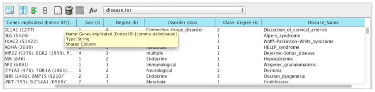
Using attribute table to verify data were imported correctly.

We can overlay the network with the attributes using visual styles:

• 42Click on the ‘Style’ tab to edit your visual styles.
• 43Click on the ‘Node’ tab to reveal Node properties.
• 44Click on the ‘Properties’ drop down and click on ‘Show All’.
• 45Scroll to ‘Fill Color’. In the ‘Column’ field, choose ‘Disorder class’, and then choose ‘Discrete Mapping’.
• 46Since the network contains many disease classes, we can right click and choose ‘Mapping Value Generators → Random Color’ in the popup menu. Each disease class is then automatically assigned a random color as node fill.
• 47Click on the ‘Edge’ tab. Click on the ‘Properties’ button and click on ‘Show All’. Find the ‘Width’ field, and choose Weight for the ‘Column’ field. This value indicates how many gene mutations different diseases share. Choose Discrete Mapping, right click to activate popup menu, choose ‘Mapping Value Generators’, and choose ‘Number Series’. Set the start width to 1, and set the increment to 3. The network should look like Figure 15. Disorders that are connected with thick edges indicate more shared number of genetic mutations. For example, the ‘Leigh_syndrome’ is closely connected to ‘mitochondrial_complex_deficiency’.
• 48Click on the ‘Node’ tab. Find ‘Label’, and choose ‘Disease_Name’. Now Disease name will be displayed in each disorder instead of disease IDs.
• 49Double Click on ‘Height’, and choose ‘Degree (k)’. Choose ‘Continuous Mapping’. Double click on the mapping bar, and drag vertical ticks to make the node size range from 30 – 300 (mapped to degree 1 – 50). Repeat this step for ‘Width’.
• 50We could now reproduce the visual style used in the poster at http://www.barabasilab.com/pubs/CCNR-ALB_Publications/200705-14_PNAS-HumanDisease/Suppl/Goh_etal_poster.pdf. Your network view should look similar to Figure 16. The two selected nodes are Leukemia and Deafness classes, respectively. Diseases in the same class tend to be placed near each other and form clusters that share similar gene mutations.

Figure 15.

Visualize closely associated human diseases using attributes and vizmapper.

Figure 16.

Fully annotated Human Disease Network (HDN).

Guidelines for Understanding Results

The protocols provided here can stand alone as methods for analyzing biological networks and also serve as a starting point for more in-depth analysis using various Cytoscape analysis and visualization apps. The two basic protocols have focused on protein-protein interaction networks, but Cytoscape has been used to explore structural networks (Morris et al., 2007; Doncheva et al., 2011), protein-protein similarity networks (Atkinson et al., 2009), and biological pathways (see the Wikipathways App, the CyKEGG Parser App, and the MetScape App (Gao et al., 2010). If the starting point is a list of genes and no source network is available, apps like the AgilentLiteratureSearch App (Vailaya et al., 2005) and GeneMANIA (Montojo et al., 2010) can provide useful starting points as well as sources for information to augment existing networks. Additional Apps are available to extend the analysis and visualization we present here and delve further into the biological meaning of the interactions – they are available with documentation at http://apps.cytoscape.org.

Basic Protocol 1 demonstrates the annotation of a protein-protein interaction network with expression data, although the approach could be used to annotate networks with a wide variety of additional data. The hierarchical clusters derived from the expression data provide just one approach to exploring this data set. For instance, critical genes and proteins tend to be hubs (nodes connected to many other nodes) or part of the shortest path through the network between two other nodes (Yu et al., 2007). Various network parameters may be calculated using Cytoscape’s built-in NetworkAnalyzer (via Tools→NetworkAnalyzer) (Doncheva et al., 2012) or through Cytoscape apps such as CentiScaPe (Scardoni et al., 2009), which calculates an even larger number of network parameters. In addition to the traditional hierarchical clustering and heat map visualization, clusterMaker2 may be used to create a co-expression network where the edges between nodes represent expression profile similarities. The resulting similarity network can be further clustered to partition the network into “modules” of genes with similar expression patterns.

To explore the concept of modules in more detail, Cytoscape apps such as jActiveModules (Ideker et al., 2002) can be used to find subnetworks where nodes show significant changes in expression levels. Unlike the co-expression network approach mentioned above, jActiveModules takes the network topology into account. This can highlight subnetworks where the genes in that subnetwork experience similar expression patterns. A plausible biological explanation for co-expression of genes or proteins is functional relatedness. This is especially true in prokaryotes, where functionally-related genes may be organized into the same operons in the genome. Genes involved in a complex can exhibit just-in-time assembly, where one highly regulated critical gene controls the overall activity of the entire complex (de Lichtenberg et al., 2005) Comparing different expression patterns across experimental conditions can also reveal different mechanisms that cause the same end result. As we saw, the BiNGO app finds significantly over-represented Gene Ontology terms annotated to the genes of interest. This helps identify functions enriched in a set of genes, including sets of genes that are co-expressed.

Basic Protocol 2 demonstrates the workflow of using Cytoscape to visualize and annotate large biomedical networks. One important and useful Cytoscape feature is its Style Manager (formerly called VizMapper), which allows researchers to translate a variety of attribute data, such as gene expression profiles, functional gene groups and pathways, and protein-protein interaction types, to intuitive graphic representations that facilitate exploratory knowledge discovery. In our examples, we used BiNGO, clusterMaker and MCODE to identify closely associated gene and protein clusters. These clusters can be immediately visualized in the Network view, which is especially helpful for visualizing and understanding the local topologies and functional features in very large networks such as the Human Disease Network having thousands of nodes and edges. The Cytoscape App store contains many other examples (http://apps.cytoscape.org/apps/with_tag/datavisualization) tailored for visualizing data from various biological sources.

In our protocol, we imported disease network and additional annotation data containing disease categories, and utilize such information to aid network visualization. Such data can also be imported directly from many external sources. As mentioned above, there are many other Cytoscape 3 apps that enables data importing from data repositories such as Reactome (Joshi-Tope and Gillespie, 2005), KEGG (Kanehisa, 2002), WikiPathways (Kelder et al., 2012), MetScape (Karnovsky et al., 2012), Agilent Literature Search (Vailaya et al., 2005). Using Cytoscape, users can also integrate their own experimental data with existing network data and functional annotations.

Commentary

Background Information

The term biological network usually refers to two types of data: those human-curated from the literature and those that are experimentally derived. The former is built on curated and verified knowledge such as those stored in pathway and protein interaction databases. The latter is derived from experiments, such as protein interaction screens or gene expression correlations. Combining these two data sources and other functional annotations enables researchers to support their experiment and identify new patterns from the data. Visual exploration tools are required for this, especially if the data are large.

The omics era has brought many opportunities and challenges for network analysis. The sharp decline in the cost of high-throughput technology has made it possible to efficiently measure tens of thousands of molecular profiles at once, for hundreds of different sample groups and experimental conditions. Such rich repositories of experimental data, along with the human curated annotations from the literature, enable researchers to quickly identify novel connections between their observations and existing knowledge, thereby enabling testing of new hypotheses. In addition to the traditional genomics, transcriptomics and proteomics, accurate metabolomics, phenomics, lipidomics are also becoming more accessible. Together, these data offer different snapshots of a target organism. Even though robust and scalable computational and statistical methods have been developed to mine new signals, it is often difficult for the researcher to explore such data without high-performance, versatile and interactive visualization software.

Cytoscape was originally designed as a simple tool to visualize networks with hundreds, or maybe a few thousands, of nodes. Thanks to the continuous community support, it has expanded its capabilities and scope to handle bigger, more complex data and evolved into a sophisticated platform that can be used for many network analysis purposes. New features include:

• improved performance of network layouts and visualizations of very large networks (using edge curving and bundling to reduce edge clutter),

• flexible and fast search functions that enable the user to quickly find sets of nodes or edges with custom criteria (such as a molecular function GO term),

• connectivity to many external data repositories (e.g., Pathway Commons, Reactome),

• a more user-friendly online/local App management mechanism,

• a new network property table that supports complex annotations from a variety of sources,

• comprehensive support for many network formats for import/export,

• and a metanode (subnetwork) mechanism that enables the user to build hierarchy in a network (a network can be a node in another network), enabling a ‘high level’, ‘functional’ or ‘structural’ view of big networks (instead of a ‘flat’ hairball of tens of thousands of nodes or edges).

With these new capabilities, users can:

• explore a network obtained from experiments or annotations in Cytoscape,

• overlay the nodes or edges with experimental values (using Styles),

• obtain additional functional annotation from external sources such as Gene Ontology (GO),

• partition the network for potential functional modules (e.g. using MCODE or clusterMaker Apps),

• or merge a network with existing curated networks (e.g. using Michigan Molecular Interaction, MiMI or GeneMANIA databases).

Our protocols above demonstrate common workflows, though many other workflows are possible. New protocols are regularly posted at http://tutorials.cytoscape.org. Also, new Apps are regularly posted to the Cytoscape App store, many enabling new workflows. A good way to find popular Apps is to rank all Apps by popularity (Number of downloads) on the App store website. From the App store homepage, click ‘All Apps’ at the top left, then click the ‘downloads’ button at the top to sort Apps by number of downloads.

Critical Parameters and Troubleshooting

Out of memory errors

Symptoms

When loading a network from either a database source or from a Cytoscape session file, a “loading” message box is displayed, the progress animation continues, but no network is displayed either in the Networks tab or a network window. The Memory button in the lower right of the Cytoscape window contains “Low” instead of “OK”.

Possible causes

Cytoscape has run out of memory to load the network, or the operating system is swapping RAM to the hard disk because your Cytoscape.vmoptions file allocates more RAM to Java than your workstation has.

Remedies

Add more memory, then register the new memory with Cytoscape per the Note on Memory Consumption section of the Cytoscape user manual. If you have installed 32 bit Java and 32 bit Cytoscape, and already have 4GB of RAM, consider using 64 bit Java, 64 bit Cytoscape, adding more RAM.

Mismatch between Java and Cytoscape

Symptoms

When starting Cytoscape on Windows, you receive messages indicating that the JMV could not be found, is defective, or the maximum heap size is too large.

Possible causes

You may have inadvertently installed 32 bit Java, which is the default download from java.com on all Windows systems. If you have installed a 64 bit Cytoscape, the 32 bit Java is inappropriate.

Remedies

Uninstall 32 bit Java and install 64 bit Java instead. Oracle maintains the latest Java at http://java.com/en/download/manual.jsp. When you restart Cytoscape, you should see its splash screen.

Cytoscape Freezes during Startup

Symptoms

When starting Cytoscape, the splash screen appears and nothing more happens, or it shows the names of Cytoscape modules being loaded, but then freezes before showing a Cytoscape window.

Possible causes

Cytoscape and its code cache may have become unsynchronized, possibly as a result of installing a newer or older Cytoscape. Alternatively, a new Cytoscape installation could be taking extra time (up to 3 minutes) to build its code cache.

Remedies

If a Cytoscape windows hasn’t appeared after 3 minutes, use your OS to terminate the executing Cytoscape, then delete the Cytoscape cache directory maintained in your user directory at <userdir>/CytoscapeConfiguration/3. (For user Bob using Windows 7, the directory would be C:\Users\Bob\CytoscapeConfiguration\3). If restarting Cytoscape fails in the same way, delete the Apps, too, by removing <userdir>/CytoscapeConfiguration and restarting Cytoscape again.

No View Window after Large Network Load

Symptoms

After loading a large network, the network name appears in the Network tab, but there is no window showing the network.

Possible causes

For large networks, Cytoscape shortens the overall load time by not drawing the network view window.

Remedies

Right click on the network in the Network tab, and choose the Create View menu item. The network window will appear within a few seconds. You can create a more manageable subnetwork by using the procedure in Step 14 of Basic Protocol 1.

Data Integration Errors

Symptoms

Expression or attribute data files are not properly integrated with the loaded network.

Possible causes

The gene identifier columns that synchronize the two files do not match exactly, or the files may not be in the correct format.

Remedies

Use the Node Table or Edge Table tabs in the Table Panel to check that the network identifiers match the identifiers in the expression or attribute data file per the tutorial at http://opentutorials.cgl.ucsf.edu/index.php/Tutorial:Network_Loading_And_ID_Mapping

LITERATURE CITED

- Atkinson HJ, et al. Using sequence similarity networks for visualization of relationships across diverse protein superfamilies. PLoS One. 2009;4:e4345. doi: 10.1371/journal.pone.0004345. [DOI] [PMC free article] [PubMed] [Google Scholar]
- Bader GD, et al. BIND--The Biomolecular Interaction Network Database. Nucleic Acids Res. 2001;29:242–5. doi: 10.1093/nar/29.1.242. [DOI] [PMC free article] [PubMed] [Google Scholar]
- Bader GD, Hogue CWV. An automated method for finding molecular complexes in large protein interaction networks. BMC Bioinformatics. 2003;4:2. doi: 10.1186/1471-2105-4-2. [DOI] [PMC free article] [PubMed] [Google Scholar]
- Barrett T, et al. NCBI GEO: mining tens of millions of expression profiles—database and tools update. Nucleic acids. 2007 doi: 10.1093/nar/gkl887. [DOI] [PMC free article] [PubMed] [Google Scholar]
- Bastian M, et al. Gephi: an open source software for exploring and manipulating networks. ICWSM 2009
- Batagelj V, Mrvar A. Pajek-program for large network analysis. Connections 1998 [Google Scholar]
- Chatr-Aryamontri A, et al. The BioGRID interaction database: 2013 update. Nucleic Acids Res. 2012;41:D816–23. doi: 10.1093/nar/gks1158. [DOI] [PMC free article] [PubMed] [Google Scholar]
- Csardi G, Nepusz T. The igraph software package for complex network research. InterJournal, Complex Syst 2006 [Google Scholar]
- Doncheva NT, et al. Analyzing and visualizing residue networks of protein structures. Trends Biochem Sci. 2011;36:179–82. doi: 10.1016/j.tibs.2011.01.002. [DOI] [PubMed] [Google Scholar]
- Doncheva NT, et al. Topological analysis and interactive visualization of biological networks and protein structures. Nat Protoc. 2012;7:670–85. doi: 10.1038/nprot.2012.004. [DOI] [PubMed] [Google Scholar]
- Dutkowski J, et al. NeXO Web: the NeXO ontology database and visualization platform. Nucleic Acids Res. 2014;42:D1269–74. doi: 10.1093/nar/gkt1192. [DOI] [PMC free article] [PubMed] [Google Scholar]
- Dutkowski J, Kramer M. A gene ontology inferred from molecular networks. Nat. 2012 doi: 10.1038/nbt.2463. [DOI] [PMC free article] [PubMed] [Google Scholar]
- Dutot A, et al. GraphStream: A Tool for bridging the gap between Complex Systems and Dynamic Graphs. In, Emergent Properties in Natural and Artificial Complex Systems. Satellite Conference within the 4th European Conference on Complex Systems ECCS’2007.2007. [Google Scholar]
- Edgar R, et al. Gene Expression Omnibus: NCBI gene expression and hybridization array data repository. Nucleic Acids Res. 2002;30:207–10. doi: 10.1093/nar/30.1.207. [DOI] [PMC free article] [PubMed] [Google Scholar]
- Fisher D, et al. Analysis and Visualization of Network Data Using JUNG. J Stat 2005 [Google Scholar]
- Franceschini A, et al. STRING v9.1: protein-protein interaction networks, with increased coverage and integration. Nucleic Acids Res. 2013;41:D808–15. doi: 10.1093/nar/gks1094. [DOI] [PMC free article] [PubMed] [Google Scholar]
- Gao J, et al. Metscape: a Cytoscape plug-in for visualizing and interpreting metabolomic data in the context of human metabolic networks. Bioinformatics. 2010;26:971–3. doi: 10.1093/bioinformatics/btq048. [DOI] [PMC free article] [PubMed] [Google Scholar]
- Gasch AP, et al. Genomic Expression Programs in the Response of Yeast Cells to Environmental Changes. Mol Biol Cell. 2000;11:4241–4257. doi: 10.1091/mbc.11.12.4241. [DOI] [PMC free article] [PubMed] [Google Scholar]
- Goel R, et al. Human Protein Reference Database and Human Proteinpedia as resources for phosphoproteome analysis. Mol Biosyst. 2012;8:453–63. doi: 10.1039/c1mb05340j. [DOI] [PMC free article] [PubMed] [Google Scholar]
- Goh K-I, et al. The human disease network. Proc Natl Acad Sci U S A. 2007;104:8685–90. doi: 10.1073/pnas.0701361104. [DOI] [PMC free article] [PubMed] [Google Scholar]
- Hamosh A, et al. Online Mendelian Inheritance in Man OMIM, a knowledgebase of human genes and genetic disorders. Nucleic Acids Res. 2005;33:D514–7. doi: 10.1093/nar/gki033. [DOI] [PMC free article] [PubMed] [Google Scholar]
- Ideker T, et al. Discovering regulatory and signalling circuits in molecular interaction networks. Bioinformatics. 2002;18(Suppl 1):S233–40. doi: 10.1093/bioinformatics/18.suppl_1.s233. [DOI] [PubMed] [Google Scholar]
- Joshi-Tope G, Gillespie M. Reactome: a knowledgebase of biological pathways. Nucleic acids. 2005 doi: 10.1093/nar/gki072. [DOI] [PMC free article] [PubMed]
- Kanehisa M. The KEGG database. Novartis Found Symp. 2002;247:91–101. discussion 101–3, 119–28, 244–52. [PubMed] [Google Scholar]
- Karnovsky A, et al. Metscape 2 bioinformatics tool for the analysis and visualization of metabolomics and gene expression data. 2012 doi: 10.1093/bioinformatics/btr661. [DOI] [PMC free article] [PubMed] [Google Scholar]
- Kelder T, et al. WikiPathways: building research communities on biological pathways. Nucleic Acids Res. 2012;40:D1301–7. doi: 10.1093/nar/gkr1074. [DOI] [PMC free article] [PubMed] [Google Scholar]
- Kerrien S, et al. The IntAct molecular interaction database in 2012. Nucleic Acids Res. 2012;40:D841–6. doi: 10.1093/nar/gkr1088. [DOI] [PMC free article] [PubMed] [Google Scholar]
- De Lichtenberg U, et al. Comparison of computational methods for the identification of cell cycle-regulated genes. Bioinformatics. 2005;21:1164–71. doi: 10.1093/bioinformatics/bti093. [DOI] [PubMed] [Google Scholar]
- Lotia S, et al. Cytoscape app store. Bioinformatics. 2013;29:1350–1. doi: 10.1093/bioinformatics/btt138. [DOI] [PMC free article] [PubMed] [Google Scholar]
- Maere S, et al. BiNGO: a Cytoscape plugin to assess overrepresentation of gene ontology categories in biological networks. Bioinformatics. 2005;21:3448–9. doi: 10.1093/bioinformatics/bti551. [DOI] [PubMed] [Google Scholar]
- Margolin AA, et al. Reverse engineering cellular networks. Nat Protoc. 2006;1:662–71. doi: 10.1038/nprot.2006.106. [DOI] [PubMed] [Google Scholar]
- Merico D, et al. How to visually interpret biological data using networks. Nat Biotechnol. 2009;27:921–4. doi: 10.1038/nbt.1567. [DOI] [PMC free article] [PubMed] [Google Scholar]
- Montojo J, et al. GeneMANIA Cytoscape plugin: fast gene function predictions on the desktop. Bioinformatics. 2010;26:2927–8. doi: 10.1093/bioinformatics/btq562. [DOI] [PMC free article] [PubMed] [Google Scholar]
- Morris JH, et al. clusterMaker: a multi-algorithm clustering plugin for Cytoscape. BMC Bioinformatics. 2011;12:436. doi: 10.1186/1471-2105-12-436. [DOI] [PMC free article] [PubMed] [Google Scholar]
- Morris JH, et al. structureViz: linking Cytoscape and UCSF Chimera. Bioinformatics. 2007;23:2345–7. doi: 10.1093/bioinformatics/btm329. [DOI] [PubMed] [Google Scholar]
- Saito R, et al. A travel guide to Cytoscape plugins. Nat Methods. 2012;9:1069–76. doi: 10.1038/nmeth.2212. [DOI] [PMC free article] [PubMed] [Google Scholar]
- Scardoni G, et al. Analyzing biological network parameters with CentiScaPe. Bioinformatics. 2009;25:2857–9. doi: 10.1093/bioinformatics/btp517. [DOI] [PMC free article] [PubMed] [Google Scholar]
- Shannon P, et al. Cytoscape: a software environment for integrated models of biomolecular interaction networks. Genome Res. 2003;13:2498–504. doi: 10.1101/gr.1239303. [DOI] [PMC free article] [PubMed] [Google Scholar]
- Su G, et al. GLay: community structure analysis of biological networks. Bioinformatics. 2010;26:3135–7. doi: 10.1093/bioinformatics/btq596. [DOI] [PMC free article] [PubMed] [Google Scholar]
- Tarcea VG, et al. Michigan molecular interactions r2: from interacting proteins to pathways. Nucleic Acids Res. 2009;37:D642–6. doi: 10.1093/nar/gkn722. [DOI] [PMC free article] [PubMed] [Google Scholar]
- Turinsky AL, et al. In: Structural Genomics. Chen YW, editor. Humana Press; Totowa, NJ: 2014. [Google Scholar]
- Vailaya A, et al. An architecture for biological information extraction and representation. Bioinformatics. 2005;21:430–8. doi: 10.1093/bioinformatics/bti187. [DOI] [PubMed] [Google Scholar]
- Yu H, et al. The importance of bottlenecks in protein networks: correlation with gene essentiality and expression dynamics. PLoS Comput Biol. 2007;3:e59. doi: 10.1371/journal.pcbi.0030059. [DOI] [PMC free article] [PubMed] [Google Scholar]
- Zuberi K, et al. GeneMANIA prediction server 2013 update. Nucleic Acids Res. 2013;41:W115–22. doi: 10.1093/nar/gkt533. [DOI] [PMC free article] [PubMed] [Google Scholar]