Genome-Wide Regression and Prediction with the BGLR Statistical Package

Abstract

Many modern genomic data analyses require implementing regressions where the number of parameters (p, e.g., the number of marker effects) exceeds sample size (n). Implementing these large-p-with-small-n regressions poses several statistical and computational challenges, some of which can be confronted using Bayesian methods. This approach allows integrating various parametric and nonparametric shrinkage and variable selection procedures in a unified and consistent manner. The BGLR R-package implements a large collection of Bayesian regression models, including parametric variable selection and shrinkage methods and semiparametric procedures (Bayesian reproducing kernel Hilbert spaces regressions, RKHS). The software was originally developed for genomic applications; however, the methods implemented are useful for many nongenomic applications as well. The response can be continuous (censored or not) or categorical (either binary or ordinal). The algorithm is based on a Gibbs sampler with scalar updates and the implementation takes advantage of efficient compiled C and Fortran routines. In this article we describe the methods implemented in BGLR, present examples of the use of the package, and discuss practical issues emerging in real-data analysis.

MANY modern statistical learning problems involve the analysis of high-dimensional data; this is particularly common in genetic studies where, for instance, phenotypes are regressed on large numbers of predictor variables (e.g., SNPs) concurrently. Implementing these large-p-with-small-n regressions (where n denotes sample size and p represents the number of predictors) poses several statistical and computational challenges, including how to confront the so-called “curse of dimensionality” (Bellman 1961) as well as the complexity of a genetic mechanism that can involve various types and orders of interactions. Recent developments in shrinkage and variable selection estimation procedures have made the implementation of these large-p-with-small-n regressions feasible. Consequently, whole-genome-regression approaches (Meuwissen et al. 2001) are becoming increasingly popular for the analysis and prediction of complex traits in plants (e.g., Crossa et al. 2010), animals (e.g., Hayes et al. 2009, VanRaden et al. 2009), and humans (e.g., Yang et al. 2010; Makowsky et al. 2011; Vazquez et al. 2012; de los Campos et al. 2013b).

In the past decade a large collection of parametric and nonparametric methods have been proposed and empirical evidence has demonstrated that no single approach performs best across data sets and traits. Indeed, the choice of the model depends on multiple factors such as the genetic architecture of the trait, marker density, sample size and the span of linkage disequilibrium (e.g., de los Campos et al. 2013a). Although various software (BLR, Pérez et al. 2010; rrBLUP, Endelman 2011; synbreed, Wimmer et al. 2012; GEMMA, Zhou and Stephens 2012) exist, most statistical packages implement a few types of methods and the integration of these methods in a unified statistical and computational framework is needed. Motivated by this we have developed the R (R Core Team 2014) package BGLR. The package offers the user great latitude in combining different methods into models for data analysis and is available at CRAN (http://cran.at.r-project.org/web/packages/BGLR/index.html) and at the R-forge website (https://r-forge.r-project.org/projects/bglr/). In this article we discuss the statistical models implemented in BGLR (Statistical Models, Algorithms, and Data), present several examples based on real and simulated data (Application Examples), and provide benchmarks of computational time and memory usage for a linear model (Benchmark of Parametric Models). All the examples and benchmarks presented in this article are based on BGLR version 1.0.3. In addition to the scripts presented in the boxes included this article we provide supplementary code in File S1, and text version of all the scripts used to produce the results presented in the article in File S2.

Statistical Models, Algorithms, and Data

The BGLR package supports models for continuous (censored or not) and categorical (binary or ordinal multinomial) traits. We first describe the models implemented in BGLR using a continuous, uncensored, response as example. Further details about censored and categorical outcomes are provided later on this article and in the supporting information, File S1.

For a continuous response (y_i; i = 1, …, n) the data equation is represented as y_i = η_i + ε_i, where η_i is a linear predictor (the expected value of y_i given predictors) and ε_i are independent normal model residuals with mean zero and variance $w_i^2{\sigma }_{\epsilon }^2$. Here, the $w_i^{\prime }s$ are user-defined weights (by default BGLR sets w_i = 1 for all data-points) and ${\sigma }_{\epsilon }^2$ is a residual variance parameter. In matrix notation we have

$$y=\eta +\mathit{\epsilon },$$

where y = {y₁, …, y_n}, η = {η₁, …, η_n}, and ε = {ε₁, …, ε_n}.

The linear predictor represents the conditional expectation function, and it is structured as

$$\eta =1\mu +{\displaystyle \sum _{j=1}^J{X}_j{\mathit{\beta }}_j}+{\displaystyle \sum _{l=1}^L{u}_l},$$ (1)

where μ is an intercept, X_j are design matrices for predictors, X_j = {x_ijk}, β_j are vectors of effects associated to the columns of X_j, and u_l = {u_l1, …, u_ln} are vectors of random effects. The only element of the linear predictor included by default is the intercept. The other elements are user specified. Collecting the above assumptions, we have the following conditional distribution of the data:

$$p\left(y|\mathit{\theta }\right)={\displaystyle \prod _{i=1}^{n}N\left(y_i|\mu +{\displaystyle \sum _{j=1}^J{\displaystyle \sum _{k=1}^{K_j}{x}_{ijk}{\beta }_{jk}}}+{\displaystyle \sum _{l=1}^L{u}_{li},{\sigma }_{\epsilon }^2{w}_i^2}\right)},$$

where θ represents the collection of unknowns, including the intercept, regression coefficients, other random effects, and the residual variance.

Prior density

The prior density is assumed to admit the following factorization:

$$p\left(\theta \right)=p\left(\mu \right)p\left({\sigma }_{\epsilon }^2\right){\displaystyle \prod _{j=1}^J}p\left({\beta }_j\right){\displaystyle \prod _{l=1}^L}p\left(u_l\right).$$

The intercept is assigned a flat prior and the residual variance is assigned a scaled-inverse χ² density $p\left({\sigma }_{\epsilon }^2\right)={\chi }^{-2}\left({\sigma }_{\epsilon }^2|S_{\epsilon },{\text{df}}_{\epsilon }\right)$ with degrees of freedom df_ε(> 0) and scale parameter S_ε(> 0). In the parameterization used in BGLR, the prior expectation of the scaled-inverse χ² density χ⁻²(⋅|S., df) is given by $S./\left(\text{df}-2\right)$.

Regression coefficients {β_jk} can be assigned either uninformative (i.e., flat) or informative priors. Those coefficients assigned flat priors, the so-called “fixed” effects, are estimated based on information contained in the likelihood solely. For the coefficients assigned informative priors, the choice of the prior plays an important role in determining the type of shrinkage of estimates of effects induced. Figure 1 provides a graphical representation of the prior densities available in BGLR. The Gaussian prior induces shrinkage of estimate similar to that of ridge regression (RR; Hoerl and Kennard 1970), where all effects are shrunk to a similar extent; we refer to this model as the Bayesian ridge regression (BRR). The scaled-t and double exponential (DE) densities have higher mass at zero and thicker tails than the normal density. These priors induces a type of shrinkage of estimates that is size-of-effect dependent (Gianola 2013). The scaled-t density is the prior used in model BayesA (Meuwissen et al. 2001), and the DE or Laplace prior is the one used in the BL (Park and Casella 2008). Finally, BGLR implements two finite mixture priors: a mixture of a point of mass at zero and a Gaussian slab, a model referred to in the literature on genomic selection (GS) as BayesC (Habier et al. 2011), and a mixture of a point of mass at zero and a scaled-t slab, a model known in the GS literature as BayesB (Meuwissen et al. 2001). By assigning a nonnull prior probability for the marker effect to be equal to zero, the priors used in BayesB and BayesC have potential for inducing variable selection.

Figure 1.

Prior densities of regression coefficients implemented in BGLR (all densities in the figure have null mean and unit variance).

Hyperparameters:

Each of the prior densities described above are indexed by one or more parameters that control the type and extent of shrinkage/variable selection induced. We treat most of these regularization parameters as random; consequently a prior is assigned to these unknowns. Table 1 lists, for each of the prior densities implemented, the set of hyperparameters. Further details about how regularization parameters are inferred from the data are given in the supporting information, File S1.

Table 1. Prior densities available for regression coefficients in the BGLR package.

Model (prior density)	Hyperparameters	Treatment in BGLRa
Flat (FIXED)	Mean (μβ)	μβ = 0
	Variance $\left({\sigma }_{\beta }^2\right)$	${\sigma }_{\beta }^2=1\times 1^{10}$
Gaussian (BRR)	Mean (μβ)	μβ = 0
	Variance $\left({\sigma }_{\beta }^2\right)$	${\sigma }_{\beta }^2\sim {\chi }^{-2}$
Scaled-t (BayesA)	Degrees of freedom (dfβ)	User specified (default value, 5)
	Scale (Sβ)	Sβ ∼ Gamma
Double exponential (BL)	λ2	λ fixed, user specified, or λ2 ∼ Gamma, or $\lambda /\max \sim Beta$b
Gaussian mixture (BayesC)	π (prop. of nonnull effects)	π ∼ Beta
	dfβ	User specified (default value, 5)
	Sβ	Sβ ∼ Gamma
Scaled-t mixture (BayesB)	π (prop. of nonnull effects)	π ∼ Beta
	dfβ	User specified (default value, 5)
	Sβ	Sβ ∼ Gamma

^aFurther details are given in the supporting information (Section A of File S1).

^bThis approach is further discussed in de los Campos et al. (2009b).

Combining priors:

Different priors can be specified for each of the set of coefficients of the linear predictor, {β₁, …, β_J, u₁, u₂, …, u_L}, giving the user great flexibility in building models for data analysis; an example illustrating how to combine different priors in a model is given in Example 2 of Application Examples.

Gaussian processes:

The vectors of random effects u_l are assigned multivariate-normal priors with a mean equal to zero and covariance matrix $\text{Cov}\left(u_l,u_l^{\prime }\right)=K_l{\sigma }_{ul}^2$, where K_l is a (user-defined) n × n-symmetric positive semidefinite matrix and ${\sigma }_{ul}^2$ is a variance parameter with prior density ${\sigma }_{ul}^2\sim {\chi }^{-2}\left({\text{df}}_l,S_l\right)$. These random effects can be used to deal with different types of problems, including but not limited to: (a) regressions on pedigree (Henderson 1975), (b) genomic BLUP (VanRaden 2008), and (c) nonparametric genomic regressions based on reproducing kernel Hilbert spaces (RKHS) methods (e.g., de los Campos et al. 2009a, 2010; Gianola et al. 2006). Examples about the inclusion of these Gaussian processes into models for data analysis are given in Application Examples.

Categorical Response

The argument response_type is used to indicate BGLR whether the response should be regarded as gaussian, the default value, or ordinal. For continuous traits the response vector should be coercible to numeric; for ordinal traits the response can take on K possible (ordered) values y_i ∈ {1, …, K} (the case where K = 2 corresponds to the binary outcome), and the response vector should be coercible to a factor. For categorical traits we use the probit link; here, the probability of each of the categories is linked to the linear predictor according to the following link function

$$P\left(y_i=k\right)=\Phi \left({\eta }_i-{\gamma }_k\right)-\Phi \left({\eta }_i-{\gamma }_{k-1}\right),$$

where Φ(⋅) is the standard normal cumulative distribution function, η_i is the linear predictor, specified as described above, and γ_k are threshold parameters, with γ₀ = −∞, γ_k ≥ γ_k−1, γ_K = ∞. The probit link is implemented using data augmentation (Tanner and Wong 1987); this is done by introducing a latent variable (so-called liability) l_i = η_i + ε_i and a measurement model y_i = k if γ_k−1 ≤ l_i ≤ γ_k. For identification purpouses, the residual variance is set equal to one. At each iteration of the Gibbs sampler the unobserved liability scores are sampled from truncate normal densities; once the unobserved liability has been sampled, the Gibbs sampler proceeds as if l_i were observed (see Albert and Chib 1993, for further details).

Missing Values

The response vector can contain missing values. Internally, at each iteration of the Gibbs sampler, missing values are sampled from the corresponding fully conditional density. Missing values in predictors are not allowed.

Censored Data

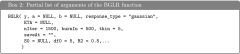
Censored data in BGLR is described using a triplet {a_i, y_i, b_i}, the elements of which must satisfy a_i < y_i < b_i. Here, y_i is the observed response (e.g., a time-to-event variable, observable only in uncensored data points, otherwise missing, NA) and a_i and b_i define lower and upper bounds for the response, respectively. Table 2 gives the configuration of the triplet for the different types of data points. The triplets are provided to BGLR in the form of three vectors (y, a, b). The vectors a and b have NULL as default value; therefore, if only y is provided this is interpreted as a continuous trait without censoring. If a and b are provided together with y, data are treated as censored. Censoring is dealt with as a missing data problem; at each iteration of the MCMC algorithm the missing values of y_i, present due to censoring, are sampled from truncated normal densities that satisfy a_i < y_i < b_i. An example of how to fit models for censored data are given in the supporting information in File S1 (Section E).

Table 2. Configuration of the triplet used to described censored data points in BGLR.

Type of point	ai	yi	bi
Uncensored	NULL	yi	NULL
Right censored	ai	NA	Inf
Left censored	−Inf	NA	bi
Interval censored	ai	NA	bi

Algorithms

The R-package BGLR draws samples from the posterior density using a Gibbs sampler (Geman and Geman 1984; Casella and George 1992) with scalar updating. For computational convenience the scaled-t and DE densities are represented as infinite mixtures of scaled normal densities (Andrews and Mallows 1974), and the finite-mixture priors are implemented using latent random Bernoulli variables linking effects to components of the mixtures. The computationally demanding steps are performed using compiled C and Fortran code.

User Interface

The R-package BGLR has a user interface similar to that of BLR (Pérez et al. 2010); however, we have modified key elements of the interface, and the internal implementation, to provide the user with greater flexibility for model building. All the arguments of the BGLR function have default values, except the vector of phenotypes. Therefore, the simplest call to the BGLR program is as follows.

When the call fm<-BGLR(y = y) is made, BGLR fits an intercept model, a total of 1500 cycles of a Gibbs sampler (the default value for the number of iterations; see Box 2) are run, and the first 500 samples are discarded, this is the default value for burn-in (see Box 2). As the Gibbs sampler collects samples, some are saved to the hard drive (only the most recent samples are retained in memory) in files with extension ∗.dat, and the running means required for computing estimates of the posterior means and of the posterior standard deviations are updated; by default, a thinning of 5 is used but this can be modified by the user using the thin argument of BGLR. Once the iteration process finishes, BGLR returns a list with estimates and the arguments used in the call.

Inputs

Box 2, displays a list of the main arguments of the BGLR function, a short description follows:

• y, a, b (y, coercible to either numeric or factor, a and b of type numeric) and response_type (character) are used to define the response.

• ETA (of type list) is used to specify the linear predictor. By default it is set to NULL, in which case only the intercept is included. Further details about the specification of this argument are given below.

• nIter, burnIn, and thin (all of type integer) control the number of iterations of the sampler, the number of samples discarded, and the thinning used to compute posterior means, respectively.

• saveAt (character) can be used to indicate BGLR where to store the samples and to provide a pre-fix to be appended to the names of the file where samples are stored. By default samples are saved in the current working directory and no pre-fix is added to the file names.

• S0, df0, R2 (numeric) define the prior assigned to the residual variance, df0 defines the degrees of freedom, and S0 defines the scale. If the scale is NULL, its value is chosen so that the prior mode of the residual variance matches the variance of phenotypes times 1-R2 (see supporting information, Section A of File S1, for further details).

Return

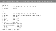
The function BGLR returns a list with estimated posterior means and estimated posterior standard deviations and the arguments used to fit the model. Box 3, shows the structure of the object returned after fitting the intercept model of Box 1. The first element of the list (y) is the response vector used in the call to BGLR, $whichNa gives the position of the entries in y that were missing, these two elements are then followed by several entries describing the call (omitted in Box 3), and this is followed by estimated posterior means and estimated posterior standard deviations of the linear predictor ($yHat and $SD.yHat), the intercept ($mu and $SD.mu), and the residual variance ($varE and $SD.varE). Finally $fit gives a list with DIC and DIC-related statistics (Spiegelhalter et al. 2002).

Output files

Box 4, shows an example of the files generated after executing the commands given in Box 1. In this case samples of the intercept (mu.dat) and of the residual variance (varE.dat) were stored. These samples can be used to assess convergence and to estimate Monte Carlo error. The R-package coda (Plummer et al. 2006) provides several useful functions for the analysis of samples used in Monte Carlo algorithms.

Data Sets

The BGLR package comes with two genomic data sets involving phenotypes, markers, pedigree, and other covariates.

Mice data set:

This data set is from the Wellcome Trust (http://gscan.well.ox.ac.uk) and has been used for detection of quantitative trait loci (QTL) by Valdar et al. (2006a,b) and for whole-genome regression by Legarra et al. (2008), de los Campos et al. (2009b), and Okut et al. (2011). The data set consists of genotypes and phenotypes of 1814 mice. Several phenotypes are available in the data frame mice.pheno. Each mouse was genotyped at 10,346 SNPs. We removed SNPs with minor allele frequency (MAF) <0.05 and imputed missing genotypes with expected values computed with estimates of allele frequencies derived from the same data. In addition to this, an additive relationship matrix (mice.A) is provided; this was computed using the R-package pedigreemm (Bates and Vazquez 2009; Vazquez et al. 2010).

Wheat data set:

This data set is from CIMMYT global wheat breeding program and comprises phenotypic, genotypic, and pedigree information of 599 wheat lines. The data set was made publicly available by Crossa et al. (2010). Lines were evaluated for grain yield (each entry corresponds to an average of two plot records) at four different environments; phenotypes (wheat.Y) were centered and standardized to a unit variance within environment. Each of the lines were genotyped for 1279 diversity array technology (DArT) markers. At each marker two homozygous genotypes were possible and these were coded as 0/1. Marker genotypes are given in the object wheat.X. Finally a matrix wheat. A provides the pedigree relationships between lines computed from the pedigree (see Crossa et al. 2010 for further details). Box 5, illustrates how to load the wheat and mice data sets.

Application Examples

In this section we illustrate the use of BGLR with various application examples, including comparison of shrinkage and variable selection methods (Example 1), how to fit models that account for genetic and nongenetic effects such as covariates or effects of the experimental design (Example 2), models for simultaneous regression on markers and pedigree (Example 3), reproducing kernel Hilbert spaces regression (Examples 4 and 5), and the assessment of prediction accuracy (Examples 6 and 7). The scripts used to fit the models discussed in each of these examples are presented in the text; additional scripts with code for post hoc analysis (e.g., plots) are provided in the supporting information (File S1 and File S2).

Example 1: Comparison of shrinkage and variable selection methods

In this example we show how to fit models that induce variable selection and others that shrink estimates toward zero. In the example, we use simulated data generated using the marker genotypes for the mice data set. We assume a very simple simulation setting with only 10 QTL. Phenotypes were simulated under the standard additive model,

$$y_i={\displaystyle \sum _{j=1}^p{x}_{ij}{\beta }_j+{\epsilon }_i},\hspace{0.5em}i=1,\dots ,n,$$

where ε_i ∼ N(0, 1 − h²), h² = 0.5. Marker effects were sampled from the mixture model:

$${\beta }_j=\{\begin{array}{ll}N\left(0,h^2/10\right)\hfill & \text{if}\hspace{0.5em}j\in \left\{517,1551,2585,3619,4653,5687,6721,7755,8789,9823\right\}\hfill \\ 0\hfill & \text{otherwise}.\hfill \end{array}$$

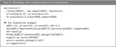
Box 6, shows the R code for simulating the phenotypes. The simulation settings can be changed using parameters that control sample size (n), the number of markers used (p), the number of QTL (nQTL), and trait heritability (h2).

Box 7, shows code that can be used to fit a Bayesian ridge regression, BayesA, and BayesB. Once the models are fitted, estimates of marker effects, predictions, estimates of the residual variance, and measures of goodness of fit and model complexity can be extracted from the object returned by BGLR. Box S1 of File S1, provides the code used to extract the results presented next.

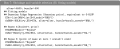
Table 3 provides the estimated residual variance, the deviance information criterion (DIC) and the effective number of parameters (pD) (Spiegelhalter et al. 2002). The estimated residual variances were all closed to the simulated value (0.5). According to pD (288.9, 200.2, 198.3 for the BRR, BayesA, and BayesB, respectively) the BRR was the most complex model, and DIC (“smaller is better”) favored BayesA and BayesB over the BRR, clearly. This was expected given the simple trait architecture simulated. Model BayesA and BayesB gave very similar estimates and predictions; this happened because in BayesB the estimated probability for the markers to have nonnull effects was very high (>0.9); as this proportion approaches one, BayesB converges to BayesA. The correlation between the true and simulated signals were high in all cases (0.86 for the BRR, 0.947 for BayesA, and 0.955 for BayesB) but favored BayesA and BayesB over the BRR, clearly. We run the simulation using 30 QTL and removing the QTL genotypes in the data analysis and the ranking of the models, based on DIC and on the correlation between predicted and simulated signal was similar to the one reported above.

Table 3. Measures of Fit and of Model Complexity.

Model	Residual variance	DIC	pD
Bayesian ridge regression	0.506 (0.020)	4200.0	288.9
BayesA	0.489 (0.019)	4047.4	200.2
BayesB	0.482 (0.019)	4017.6	198.3

Figure 2 displays the absolute values of estimates of marker effects for models BayesA (red) and the BRR (black). The estimates of BayesB (not shown) are similar to those of BayesA. The vertical lines and blue dots give the position and absolute value of the simulated effects. The BRR gives a profile of estimated of effects where all markers had tiny effects; BayesA and BayesB give a very different profiles of effects: most of the simulated QTL were detected (except the first one), markers having no effects had very small estimated effects, and QTL had sizable estimated effects. This simulation illustrates how in ideal circumstances the choice of the prior density assigned to marker effects can make a big difference in terms of estimates of effects. However, the difference between models is expected to be much smaller under more complex genetic architectures and, perhaps more importantly, when the marker panel does not contain markers in tight LD with QTL, e.g., Wimmer et al. (2013). The example also illustrates a very important concept: in high-dimensional regressions it is possible to have similar predictions with very different estimates of effects. Indeed, in the example presented above, although the correlation of effects estimated by BRR and BayesB was low (0.226), the correlation between predictions (yHat) derived from each of the models was relatively high (0.946).

Figure 2.

Absolute value of estimated marker effects (black, Bayesian ridge regression; red, BayesB; blue, simulated Value).

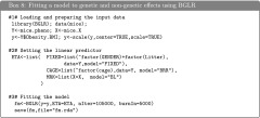
Example 2: Fitting models for genetic and nongenetic factors

In the next example we illustrate how to fit models with various sets of predictors using the mice data set. Valdar et al. (2006b) pointed out that the cage where mice were housed had an important effect in the physiological covariates and Legarra et al. (2008) and de los Campos et al. (2009b) used models that accounted for sex, litter size, cage, familial relationships, and markers. Therefore, one possible linear model that we can fit to a continuous phenotype is

$$y=1\mu +X_1{\beta }_1+X_2{\beta }_2+X_3{\beta }_3+\epsilon ,$$

where y is the phenotype vector (body mass index, in the example), μ is an intercept, X₁ is a design matrix for the effects of sex and litter size, β₁ is the corresponding vector of effects, X₂ is the design matrix for the effects of cage, β₂ is a vector of cage effects, X₃ is the matrix with marker genotypes, and β₃ is the corresponding vector of marker effects. We treat β₁ as “FIXED” and the other two vectors of effects as random; β₂ is treated as Gaussian and marker effects, β₃, are assigned IID double-exponential priors, which corresponds to the prior used in the Bayesian LASSO model.

Fitting the model:

The script needed to fit the model above described is given in Box 8. The first block of code, #1#, loads the data. In the second block of code we set the linear predictor. This is specified using a two-level list. Each of the elements of the inner list is used to specify one element of the linear predictor; these elements are specified by providing a formula or a design matrix and a prior (model argument). When the formula is used, the design matrix is created internally using the model.matrix() function of R. Additional arguments in the specification of the linear predictors are optional (see Table S1, File S1 for the arguments used to specify hyperparameters). Finally in the third block of code we fit the model by calling the BGLR() function. When BGLR begins to run, a message warns the user that hyperparameters were not provided and that consequently they were set using built-in rules (see Table S1, File S1, for further details).

Extracting results:

Once the model was fitted one can extract from the list returned by BGLR the estimated posterior means and the estimated posterior standard deviations as well as measures of model goodness of fit and model complexity. Also, as BGLR runs, it saves samples of some of the parameters; these samples can be brought into the R-environment for posterior analysis. Box S2 of File S1, illustrates how to extract estimates from the models fitted in Box 8. Some of the results are given in Figure 3. In the example, phenotypes were standardized to a unit sample variance and the estimated residual variance was 0.53, suggesting that the model explained ∼47% of the phenotypic variance. Figure 3, top left, gives the absolute value of estimated effects and Figure 3, top right, gives a scatter plot of phenotypes vs. predicted genomic values; this prediction does not include differences due to sex, litter size, or cage. Figure 3, bottom, gives trace plots of the residual variance (left) and of the regularization parameter of the Bayesian LASSO (right). The residual variance had a very good mixing; however, the mixing of the regularization parameter was not as good. In general, with large numbers of markers long chains are needed to infer regularization parameters precisely.

Figure 3.

Squared-estimated marker effects (top left), phenotype vs. predicted genomic values (top right), trace plot of residual variance (bottom left), and trace plot of regularization parameter of the Bayesian LASSO (bottom right).

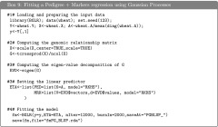
Example 3: Fitting a pedigree+markers BLUP model using BGLR

In the following example we illustrate how to incorporate in the model Gaussian random effects with user-defined covariance structures. These types of random effects appear both in pedigree and genomic models. The example presented here uses the wheat data set included with the BGLR package. In the example of Box 9 we include two random effects, one representing a regression on pedigree, $a\sim N\left(0,\hspace{0.5em}A{\sigma }_a^2\right)$, where A is a pedigree-derived numerator relationship matrix, and one representing a linear regression on markers, $g\sim N\left(0,\hspace{0.5em}G{\sigma }_g^2\right)$ where G is a marker-derived genomic relationship matrix. For ease of interpretation of estimates of variance components we standardized both matrices to an average diagonal value of (approximately) one. The implementation of Gaussian processes in BGLR exploits the equivalence between these processes and random regressions on principal components (de los Campos et al. 2010; Janss et al. 2012). The user can implement a RKHS regression either by providing covariance matrix (K) or its eigenvalue decomposition (see the example in Box 9). When the covariance matrix is provided, the eigenvalue decomposition is computed internally. Box S3 of File S1, shows how to extract estimates, predictions, and samples from the fitted model. The estimated residual variance (posterior standard deviation) was 0.43 (0.044), and the estimates of the variance components associated to the pedigree, ${\sigma }_a^2$, and markers, ${\sigma }_g^2$, were 0.24 (0.07) and 0.42 (0.09), respectively. The code in Box S3 of File S1, shows how to obtain samples of heritability from the samples collected before each of the variance components. The estimated posterior mean of the ratio of the genetic variance $\left({\sigma }_a^2+{\sigma }_g^2\right)$ relative to the total variance was 0.6; therefore, we conclude that ∼60% of the phenotypic variance can be explained by genetic factors. In this example, the pedigree explained approximately one-third of the total genetic variance and markers explained the other two-thirds. The samples from the posterior distribution of ${\sigma }_a^2$ and ${\sigma }_g^2$ had a posterior correlation of −0.184; this happens because both A and G are, to some extent, redundant.

Reproducing kernel Hilbert spaces regressions:

Reproducing Kernel Hilbert Spaces Regressions (RKHS) have been used for regression (e.g., smoothing spline, Wahba 1990), spatial smoothing (e.g., kriging, Cressie 1988), and classification problems (e.g., support vector machine, Vapnik 1998). Gianola et al. (2006) proposed using this approach for genomic prediction and since then several methodological and applied articles have been published elsewhere (Gianola and de los Campos 2008; de los Campos et al. 2009a, 2010). In this section we illustrate how to implement RKHS using single- (Example 4) and multi- (Example 5) kernel methods.

Example 4: Single-kernel models

In RKHS the regression function is a linear combination of the basis function provided by the reproducing kernel (RK); therefore, the choice of the RK constitutes one of the central elements of model specification. The RK is a function that maps from pairs of points in input space (i.e., pairs of individuals) into the real line and must be positive semidefinite. For instance, if the information set is given by vectors of marker genotypes the RK, $K\left(x_i,x_{i^{\prime }}\right)$ maps from pairs of vectors of genotypes, $\left\{x_i,x_{i^{\prime }}\right\}$ onto the real line with a map that must satisfy ${\displaystyle {\sum }_i{\displaystyle {\sum }_{i^{\prime }}{\alpha }_i{\alpha }_{i^{\prime }}K\left(x_i,x_{i^{\prime }}\right)\ge 0}}$, for any nonnull sequence of coefficients α_i. Following de los Campos et al. (2009a) the Bayesian RKHS regression can be represented as

$$y=\mathbf{1}\mu +u+\mathit{\epsilon }\hspace{0.17em}\text{with}\hspace{0.17em}p\left(\mu ,u,\mathit{\epsilon }\right)\propto N\left(u|\mathbf{0},\hspace{0.5em}K{\sigma }_u^2\right)N\left(\mathit{\epsilon }|\mathbf{0},\hspace{0.5em}I{\sigma }_{\epsilon }^2\right),$$ (2)

where $K=\left\{K\left(x_i,x_{i^{\prime }}\right)\right\}$ is an (n × n)-matrix whose entries are the evaluations of the RK at pairs of points in input space. Note that the structure of the model described by (2) is that of the standard animal model (Quaas and Pollak 1980) with the pedigree-derived numerator relationship matrix (A) replaced by the kernel matrix (K). Box 10, features an example using a Gaussian kernel evaluated in the (average) squared-Euclidean distance between genotypes, that is:

$$K\left(x_i,x_{i^{\prime }}\right)=\exp \left\{-h\times \frac{{\displaystyle {\sum }_{k=1}^p{\left(x_{ik}-x_{i^{\prime }k}\right)}^2}}{p}\right\}.$$

In the example genotypes were centered and standardized, but this is not strictly needed. The bandwidth parameter, h, controls how fast the covariance function drops as the distance between pairs of vector genotypes increases. This parameter plays an important role in inferences and predictions. In this example we have arbitrarily chosen the bandwidth parameter to be equal to 0.25; further discussion about this parameter is given in the next example. With this choice of RK, the estimated residual variance was 0.41, which suggests that the RKHS model fitted in Box 10, fits the data slightly better than the pedigree + markers models of Box 9. Box S4 of File S1, provides supplementary code for the model fitted in Box 10.

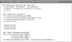
Example 5: Multikernel methods

The bandwidth parameter of the Gaussian kernel can be chosen using either cross-validation (CV) or Bayesian methods. From a Bayesian perspective, one possibility is to treat h as random; however, this is computationally demanding because the RK needs to be recomputed any time h is updated. To overcome this problem de los Campos et al. (2010) proposed using a multikernel approach (named kernel averaging, KA) consisting of: (a) defining a sequence of kernels based on a set of values of h, and (b) fitting a multikernel model with as many random effects as kernels in the sequence. The model has the form

$$y=\mathbf{1}\mu +{\displaystyle {\sum }_{l=1}^L{u}_l+\mathit{\epsilon }}\hspace{0.5em}\text{with}\hspace{0.5em}p\left(\mu ,u_1,\dots ,u_L,\mathit{\epsilon }\right)\propto {\displaystyle {\prod }_{l=1}^{L}N\left(u_l|\mathbf{0},\hspace{0.5em}{K}_l{\sigma }_{u_l}^2\right)N\left(\mathit{\epsilon }|\mathbf{0},I{\sigma }_{\epsilon }^2\right)},$$ (3)

where K_l is the RK evaluated at the lth value of the bandwidth parameter in the sequence {h₁, …, h_L}. It can be shown (e.g., de los Campos et al. 2010) that if variance components are known, the model of expression (3) is equivalent to a model with a single random effect whose distribution is $N\left(u|\mathbf{0},\hspace{0.5em}\overline{\mathbf{K}}{\sigma }_u^2\right),$ where $\overline{\mathbf{K}}$ is a weighted average of all the RK used in (3) with weights proportional to the corresponding variance components (hence the name kernel averaging). Performing a grid search for h or implementing a multikernel model requires defining a reasonable range for h. If the value of h is too small, the entries of the resulting Gaussian kernel will approach a matrix full of ones; such a kernel will be redundant with the intercept, which is included as fixed effect. On the other hand, if h is too large, the off-diagonal values of the kernel matrix will approach zero, leading to a random effect that is confounded with the error term. Therefore, in choosing values for h both extremes should be avoided. Although there is no general rule to define the values of the bandwidth parameter, one possibility is to set h to values $h=1/M\times \left\{1/5,1,5\right\},$ where M is the median squared Euclidean distance between lines (computed using off-diagonals only). With this choice, the median off-diagonals of K will be $\exp \left(-\frac{1}{5}\right)$, exp(−1) and exp(−5) for h equal to $h=\frac{1}{5}\times \frac{1}{M}$, $h=\frac{1}{M}$ and $h=\frac{5}{M}$, respectively. We use this approach in Box 11, to fit a multikernel model. The resulting entries of the RK are displayed in Figure 4. Box S5 of File S1, provides supplementary code that can be used to retrieve estimates from the model fitted in Box 11. The estimated residual variance was close to 0.3 and the estimated variance components for each of the kernels fitted were 0.62, 0.48, and 0.24 for h equal to 0.098, 0.490 and 2.450, respectively. The script provided in Box S5 of File S1, produces trace plots of variance components. The residual variance has a reasonably good mixing. The sum of the variances of the three kernels also has a reasonably good mixing; however, due to confounding between the kernels, individual variance components show a much poorer mixing.

Figure 4.

Entries of the first row of the (Gaussian) kernel matrix evaluated at three different values of the bandwidth parameter, h = 0.098, 0.490, 2.450.

Assessment of prediction accuracy:

In the previous examples we illustrated how to fit different types of models to training data; in the following section we consider two ways of assessing prediction accuracy: a single training–testing partition and multiple training–testing partitions.

Example 6: Assessment of prediction accuracy using a single training-testing partition

A simple way of assessing prediction accuracy consists of partitioning the data set into two disjoint sets: one used for model training (TRN) and one used for testing (TST). Box 12, shows code that fits a G-BLUP model in a TRN–TST setting using the wheat data set. The code randomly assigns 100 individuals to the TST set. The variable tst is a vector that indicates which data points belong to the TST data set; for these entries we introduce missing values in the phenotypic vector (see Box 12). Once the model is fitted, predictions for individuals in the TST set can be obtained typing fm$yHat[tst] in the R command line; Box S6 of File S1 gives supplementary code to the example in Box 12, including the code used to produce Figure 5 that displays observed vs. predicted phenotypes for individuals in TRN (black dots) and TST (red dots) sets. The correlation between observed phenotypes and predictions was 0.83 in the TRN set and 0.60 in the TST set, and the regression of phenotypes on predictions was 1.49 and 1.24 for the TRN and TST set, respectively.

Figure 5.

Estimated genetic values for training and testing sets. Predictions were derived using G-BLUP model (see Box 12).

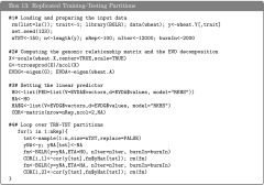
Example 7: Model comparison based on multiple training–testing partitions

The example presented in the previous section is based on a single training–testing partition. A cross-validation is simply a generalization of the single TRN–TST evaluation. For a K-fold cross-validation there are K TRN–TST partitions; in each fold, the individuals assigned to that particular fold are used for TST and the remaining individuals are used for TRN. Another possibility is to generate multiple TRN–TST partitions with random assignment of subjects to either TRN or TST. Each partition yields a point estimate of prediction accuracy (e.g., correlation between predictions and phenotypes). The variability of the point estimate across partitions (replicates) reflects uncertainty due to sampling of TRN and TST sets, and a precise estimate of prediction accuracy can be obtained by averaging the estimates of accuracy obtained in each partition.

Box 13, gives an example of an evaluation based on 100 TRN–TST partitions. In each partition two models (P, pedigree and PM, pedigree + markers) were fitted and used to predict yield in the TST data set. This yielded 100 estimates of the prediction correlation for each of the models fitted. These estimates should be regarded as paired samples because both share a common feature: the TRN–TST partition. Several statistics can be computed to compare the two models fitted, and a natural approach for testing the null hypotheses H₀: P and PM have the same prediction accuracy vs. H_A: the prediction accuracy of models P and PM are different is to conduct a paired-t-test based on the difference of the correlation coefficients. Figure 6 gives the estimated correlations for the pedigree + markers model (PM, vertical axis) vs. the pedigree-only model (P, horizontal axis) by environment. The great majority of the points lay above the 45° line indicating that in most partitions the PM model had higher prediction accuracy than the P-only model. The paired-t-test had P-values <0.001 in all environments indicating strong evidence against the null hypothesis (H₀: P and PM have the same prediction accuracy). The code used to generate the plot in Figure 6 and to carry out the t-test is given in Box S7, File S1.

Figure 6.

Estimated correlations between phenotypes and predictions in testing data sets (for a total of 100 training–testing partitions) by model (pedigree in the horizontal axis and pedigree + markers in the vertical axis) by environment (E1–E4).

Benchmark of Parametric Models

We carried out a benchmark evaluation by fitting a BRR to data sets involving three different sample size (n = 1K, 2K and 5K, K = 1000) and four different marker densities (P = 5K, 10K, 50K, and 100K). The evaluation was carried out in an Intel Xeon processor, 2 GHz, with R executed in a single thread and linked against OpenBLAS. Computing time (Figure 7) scales approximately proportional to the product of the number of records and the number of effects. For the most demanding scenario (n = 5K, P = 100K) it took ∼11 min to complete 1000 iterations of the Gibbs sampler. Using the R functions Rprof and summaryRprof we performed an analysis of memory usage. As expected the amount of memory used scaled linearly with marker density with a maximum memory usage of ∼6, 3, 0.6, and 0.3 Gb of RAM for n =5K and P = 100K, 50K, 10K, and 5K, respectively. Because R holds all the objects in virtual memory and the size of the objects depends on the underlying operating system, as a general rule, for an R session using more than 4 Gb of RAM, a 64-bit build of R would be needed.

Figure 7.

Seconds per 1000 iterations of the Gibbs sampler by number of markers and sample size. The benchmark was carried out by fitting a Gaussian regression (BRR) using an Intel Xeon processor, 2 GHz. Computations were carried out using a single thread.

Concluding Remarks

In BGLR we implemented in a unified Bayesian framework several methods commonly used in genome-enabled prediction, including various parametric models and Gaussian processes that can be used for parametric (e.g., pedigree regressions or G-BLUP) or semiparametric regressions (e.g., genomic regressions). The package supports continuous (censored or not) as well as binary and ordinal traits. The software interface gives the user great latitude in combining different modeling approaches for data analysis. In the algorithm implemented in BGLR, operations that can be vectorized are performed using built-in R-functions; however, most of the computing intensive tasks are performed using compiled routines written in C and Fortran languages. The package is also able to take advantage of multithread BLAS implementations in both Windows and UNIX-like systems. Finally, together with the package we have included two data sets and ancillary functions that can be used to read into the R-environment genotype files written in ped and bed formats (Purcell et al. 2007).

The Gibbs sampler implemented is computationally very intensive and our current implementation stores genotypes in memory; therefore, despite the effort made to make BGLR computationally efficient, performing regressions with hundreds of thousands of markers requires access to large amounts of RAM and the computational time can be considerable. Certainly, algorithms other than MCMC can be quite faster; however, the MCMC framework adopted offers great flexibility, as illustrated by the examples presented here.

Although some of the computationally intensive algorithms implemented in BGLR can benefit from multithread computing; there is room to further improve the computational performance of the software by making more intensive use of parallel computing. In future releases we plan to exploit parallel computing to a much greater extent. Also, we are currently working on modifying the software in ways that avoid loading genotypes in in memory. Future releases will be made at the R-Forge website (https://r-forge.r-project.org/R/?group_id=1525) first and, after considerable testing, at CRAN.

Literature Cited

- Albert J. H., Chib S., 1993. Bayesian analysis of binary and polychotomous response data. J. Am. Stat. Assoc. 88(422): 669–679 [Google Scholar]
- Andrews D. F., Mallows C. L., 1974. Scale mixtures of normal distributions. J. R. Stat. Soc., B 36(1): 99–102 [Google Scholar]
- Bates, D., and A. I. Vazquez, 2009 pedigreemm: pedigree-based mixed-effects models, R package version 0.2–4.
- Bellman R. E., 1961. Adaptive Control Processes: A Guided Tour. Princeton University Press, Princeton, NJ [Google Scholar]
- Casella G., George E. I., 1992. Explaining the gibbs sampler. Am. Stat. 46(3): 167–174 [Google Scholar]
- Cressie N., 1988. Spatial prediction and ordinary kriging. Math. Geol. 20(4): 405–421 [Google Scholar]
- Crossa J., de los Campos G., Pérez P., Gianola D., Burgueno J., et al. , 2010. Prediction of genetic values of quantitative traits in plant breeding using pedigree and molecular markers. Genetics 186 : 713–724 [DOI] [PMC free article] [PubMed] [Google Scholar]
- de los Campos G., Gianola D., Rosa G. J. M., 2009a Reproducing kernel Hilbert spaces regression: a general framework for genetic evaluation. J. Anim. Sci. 87(6): 1883–1887 [DOI] [PubMed] [Google Scholar]
- de los Campos G., Naya H., Gianola D., Crossa J., Legarra A., et al. , 2009b Predicting quantitative traits with regression models for dense molecular markers and pedigree. Genetics 182: 375–385 [DOI] [PMC free article] [PubMed] [Google Scholar]
- de los Campos G., Gianola D., Rosa G. J. M., Weigel K. A., Crossa J., 2010. Semi-parametric genomic-enabled prediction of genetic values using reproducing kernel Hilbert spaces methods. Genet. Res. 92: 295–308 [DOI] [PubMed] [Google Scholar]
- de los Campos G., Hickey J. M., Pong-Wong R., Daetwyler H. D., Calus M. P. L., 2013a Whole genome regression and prediction methods applied to plant and animal breeding. Genetics 193: 327–345 [DOI] [PMC free article] [PubMed] [Google Scholar]
- de los Campos G., Vazquez A. I., Fernando R. L., K. Y. C., and S. Daniel, 2013b Prediction of complex human traits using the genomic best linear unbiased predictor. PLoS Genet. 7(7): e1003608. [DOI] [PMC free article] [PubMed] [Google Scholar]
- Endelman J. B., 2011. Ridge regression and other kernels for genomic selection with r package rrblup. Plant Genome 4: 250–255 [Google Scholar]
- Geman S., Geman D., 1984. Stochastic relaxation, gibbs distributions and the Bayesian restoration of images. IEEE Trans. Pattern Anal. Mach. Intell. 6(6): 721–741 [DOI] [PubMed] [Google Scholar]
- Gianola D., 2013. Priors in whole-genome regression: the Bayesian alphabet returns. Genetics 90: 525–540 [DOI] [PMC free article] [PubMed] [Google Scholar]
- Gianola D., de los Campos G., 2008. Inferring genetic values for quantitative traits non-parametrically. Genet. Res. 90: 525–540 [DOI] [PubMed] [Google Scholar]
- Gianola D., Fernando R. L., Stella A., 2006. Genomic-assisted prediction of genetic value with semiparametric procedures. Genetics 173: 1761–1776 [DOI] [PMC free article] [PubMed] [Google Scholar]
- Habier D., Fernando R., Kizilkaya K., Garrick D., 2011. Extension of the Bayesian alphabet for genomic selection. BMC Bioinformatics 12(1): 186. [DOI] [PMC free article] [PubMed] [Google Scholar]
- Hayes B., Bowman P., Chamberlain A., Goddard M., 2009. Invited review: genomic selection in dairy cattle: progress and challenges. J. Dairy Sci. 92(2): 433–443 [DOI] [PubMed] [Google Scholar]
- Henderson C. R., 1975. Best linear unbiased estimation and prediction under a selection model. Biometrics 31(2): 423–447 [PubMed] [Google Scholar]
- Hoerl A. E., Kennard R. W., 1970. Ridge regression: biased estimation for nonorthogonal problems. Technometrics 42(1): 80–86 [Google Scholar]
- Janss L., de los Campos G., Sheehan N., Sorensen D., 2012. Inferences from genomic models in stratified populations. Genetics 192: 693–704 [DOI] [PMC free article] [PubMed] [Google Scholar]
- Legarra A., Robert-Granié C., Manfredi E., Elsen J.-M., 2008. Performance of genomic selection in mice. Genetics 180: 611–618 [DOI] [PMC free article] [PubMed] [Google Scholar]
- Makowsky R., Pajewski N. M., Klimentidis Y. C., Vazquez A. I., Duarte C. W., et al. , 2011. Beyond missing heritability: prediction of complex traits. PLoS Genet. 7(4): e1002051. [DOI] [PMC free article] [PubMed] [Google Scholar]
- Meuwissen T. H. E., Hayes B. J., Goddard M. E., 2001. Prediction of total genetic value using genome-wide dense marker maps. Genetics 157: 1819–1829 [DOI] [PMC free article] [PubMed] [Google Scholar]
- Okut H., Gianola D., Rosa G. J. M., Weigel K. A., 2011. Prediction of body mass index in mice using dense molecular markers and a regularized neural network. Genet. Res. 93: 189–201 [DOI] [PubMed] [Google Scholar]
- Park T., Casella G., 2008. The Bayesian LASSO. J. Am. Stat. Assoc. 103(482): 681–686 [Google Scholar]
- Pérez P., de los Campos G., Crossa J., Gianola D., 2010. Genomic-enabled prediction based on molecular markers and pedigree using the Bayesian Linear Regression package in R. Plant Genome 3(2): 106–116 [DOI] [PMC free article] [PubMed] [Google Scholar]
- Plummer M., Best N., Cowles K., Vines K., 2006. Coda: convergence diagnosis and output analysis for mcmc. R News 6(1): 7–11 [Google Scholar]
- Purcell S., Neale B., Todd-Brown K., Thomas L., Ferreira M. A. R., et al. , 2007. Plink: a tool set for whole-genome association and population-based linkage analyses. Am. J. Hum. Genet. 81: 559–575 [DOI] [PMC free article] [PubMed] [Google Scholar]
- Quaas R. L., Pollak E. J., 1980. Mixed model methodology for farm and ranch beef cattle testing programs. J. Anim. Sci. 51(6): 1277–1287 [Google Scholar]
- R Core Team , 2014. R: A Language and Environment for Statistical Computing. R Foundation for Statistical Computing, Vienna, Austria [Google Scholar]
- Spiegelhalter D. J., Best N. G., Carlin B. P., Van Der Linde A., 2002. Bayesian measures of model complexity and fit. J. R. Stat. Soc. Series B Stat. Methodol. 64(4): 583–639 [Google Scholar]
- Tanner M. A., Wong W. H., 1987. The calculation of posterior distributions by data augmentation. J. Am. Stat. Assoc. 82(398): 528–540 [Google Scholar]
- Valdar W., Solberg L. C., Gauguier D., Burnett S., Klenerman P., et al. , 2006a Genome-wide genetic association of complex traits in heterogeneous stock mice. Nat. Genet. 38: 879–887 [DOI] [PubMed] [Google Scholar]
- Valdar W., Solberg L. C., Gauguier D., Cookson W. O., Rawlins J. N. P., et al. , 2006b Genetic and environmental effects on complex traits in mice. Genetics 174: 959–984 [DOI] [PMC free article] [PubMed] [Google Scholar]
- VanRaden P. M., 2008. Efficient methods to compute genomic predictions. J. Dairy Sci. 91(11): 4414–4423 [DOI] [PubMed] [Google Scholar]
- VanRaden P., Tassell C. V., Wiggans G., Sonstegard T., Schnabel R., et al. , 2009. Invited review: reliability of genomic predictions for north american holstein bulls. J. Dairy Sci. 92(1): 16–24 [DOI] [PubMed] [Google Scholar]
- Vapnik V., 1998. Statistical Learning Theory, Ed. 1 Wiley, ; New York [Google Scholar]
- Vazquez A. I., Bates D. M., Rosa G. J. M., Gianola D., Weigel K. A., 2010. Technical note: an R package for fitting generalized linear mixed models in animal breeding. J. Anim. Sci. 88(2): 497–504 [DOI] [PubMed] [Google Scholar]
- Vazquez A. I., de los Campos G., Klimentidis Y. C., Rosa G. J. M., Gianola D., et al. , 2012. A comprehensive genetic approach for improving prediction of skin cancer risk in humans. Genetics 192: 1493–1502 [DOI] [PMC free article] [PubMed] [Google Scholar]
- Wahba G., 1990. Spline Models for Observational Data. Society for Industrial and Applied Mathematics, Philadelphia [Google Scholar]
- Wimmer V., Albrecht T., Auinger H.-J., Schoen C.-C., 2012. synbreed: a framework for the analysis of genomic prediction data using R. Bioinformatics 28(15): 2086–2087 [DOI] [PubMed] [Google Scholar]
- Wimmer V., Lehermeier C., Albrecht T., Auinger H.-J., Wang Y., et al. , 2013. Genome-wide prediction of traits with different genetic architecture through efficient variable selection. Genetics 195: 573–587 [DOI] [PMC free article] [PubMed] [Google Scholar]
- Yang J., Benyamin B., McEvoy B. P., Gordon S., Henders A. K., et al. , 2010. Common snps explain a large proportion of the heritability for human height. Nat. Genet. 42(7): 565–569 [DOI] [PMC free article] [PubMed] [Google Scholar]
- Zhou X., Stephens M., 2012. Genome-wide efficient mixed-model analysis for association studies. Nat. Genet. 44(7): 821–824 [DOI] [PMC free article] [PubMed] [Google Scholar]
Associated Data
This section collects any data citations, data availability statements, or supplementary materials included in this article.