

Abstract
It is crucial for researchers to optimize RNA-seq experimental designs for differential expression detection. Currently, the field lacks general methods to estimate power and sample size for RNA-Seq in complex experimental designs, under the assumption of the negative binomial distribution. We simulate RNA-Seq count data based on parameters estimated from six widely different public data sets (including cell line comparison, tissue comparison, and cancer data sets) and calculate the statistical power in paired and unpaired sample experiments. We comprehensively compare five differential expression analysis packages (DESeq, edgeR, DESeq2, sSeq, and EBSeq) and evaluate their performance by power, receiver operator characteristic (ROC) curves, and other metrics including areas under the curve (AUC), Matthews correlation coefficient (MCC), and F-measures. DESeq2 and edgeR tend to give the best performance in general. Increasing sample size or sequencing depth increases power; however, increasing sample size is more potent than sequencing depth to increase power, especially when the sequencing depth reaches 20 million reads. Long intergenic noncoding RNAs (lincRNA) yields lower power relative to the protein coding mRNAs, given their lower expression level in the same RNA-Seq experiment. On the other hand, paired-sample RNA-Seq significantly enhances the statistical power, confirming the importance of considering the multifactor experimental design. Finally, a local optimal power is achievable for a given budget constraint, and the dominant contributing factor is sample size rather than the sequencing depth. In conclusion, we provide a power analysis tool (http://www2.hawaii.edu/~lgarmire/RNASeqPowerCalculator.htm) that captures the dispersion in the data and can serve as a practical reference under the budget constraint of RNA-Seq experiments.
Keywords: RNA-Seq, sample size, power analysis, simulation, bioinformatics
INTRODUCTION
RNA-Seq is a new approach to transcriptome analysis based on next-generation sequencing (NGS) technology. It is quickly replacing microarrays as the platform for gene expression profiling, owing to the advantages of high reproducibility but low noise level. Beyond revealing gene expression patterns, the information gained from RNA-Seq has already greatly enhanced our understanding in many other areas, such as mechanisms of alternative splicing and the discovery of many novel isoforms of mRNA transcripts (Morin et al. 2008; Kim and Salzberg 2011). Furthermore, it has led to the discovery of many novel RNA transcripts, as well as the massive amount of newly discovered long intergenic noncoding RNAs (lincRNAs) relative to the small number of lincRNAs identified before RNA-Seq became popular (Morin et al. 2008; Trapnell et al. 2009; Wang et al. 2009; Kim and Salzberg 2011).
RNA-Seq data are a set of short RNA reads that are often summarized as discrete counts. The Poisson distribution had previously been used to analyze RNA-Seq data (Marioni et al. 2008; Jiang and Wong 2009; Robinson and Oshlack 2010; Srivastava and Chen 2010; Wang et al. 2010; Pham and Jimenez 2012). Several earlier RNA-Seq studies have attempted to use the Poisson distribution to perform power analysis and sample size estimation using algebraic manipulation of Wald statistics and likelihood ratio methods (Chen et al. 2011; Busby et al. 2013). Chen et al. (2011) studied several test statistics (Wald test, likelihood ratio test, Fisher's exact test, variance stabilized test, and conditional binomial test) on Poisson distribution simulations and compared their performances in terms of statistical power. They justified the use of the Poisson distribution in the simulation data by arguing that the Poisson distribution can be used when there are only technical replicates. However, the much larger variation from biologic replicates (McIntyre et al. 2011) was not addressed in the paper. Moreover, it was found that the Poisson distribution does not fit the empirical data due to the over-dispersion mainly caused by natural biological variation (Anders and Huber 2010; Robinson and Oshlack 2010). As a result, the negative binomial distribution has become widely used to analyze RNA-Seq data which allows more flexibility in assigning between-sample variations.
It is very challenging to estimate power and satisfactory sample size for the RNA-Seq differential expression (DE) tests. One issue is that analytical solutions may not always exist for RNA-Seq sample size and power calculations (McCulloch 1997; Aban et al. 2008; Pham and Jimenez 2012), due to the complexity of the negative binomial model. Instead, numerical methods such as Monte Carlo simulations have been employed to analyze the properties of negative binomial models (McCulloch 1997; Robinson and Smyth 2007; Aban et al. 2008; Srivastava and Chen 2010; Robles et al. 2012; Vijay et al. 2013). Other issues involved in power estimation include the combination of multiple hypotheses testing (MHT), P-value calculation, and various ways to estimate dispersion and normalization factors for library sizes. In RNA-Seq analysis, tens of thousands of genes are analyzed for statistical significance simultaneously. A naïve approach would analyze each individual gene independently without consideration of the entire data set. However, in reality different genes are correlated instead of being independent of each other in the same sample. Moreover, samples in the same condition are also correlated. Such information should be taken into account in order to obtain more accurate results. This strategy has been implemented in recent RNA-Seq DE packages such as DESeq, DESeq2, edgeR, EBSeq, and sSeq (Anders and Huber 2010; Robinson et al. 2010; Leng et al. 2013; Yu et al. 2013; Love et al. 2014).
Several studies examined differences between statistical packages of RNA-Seq DE analysis (Kvam et al. 2012; Nookaew et al. 2012; Robles et al. 2012; Rapaport et al. 2013). Nookaew et al. evaluated the differences in DE using the experimental data of yeasts in different growth conditions. Conversely others (Kvam et al. 2012; Robles et al. 2012; Rapaport et al. 2013; Soneson and Delorenzi 2013) calculated true positive rate (TPR) and false positive rate (FPR) using simulated data sets under varying parameters. In this report, we took a unique combination of simulated and experimental data approaches, where the parameters in the simulations were based on six different experimental data sets that span a wide range of conditions and samples. This approach is solidly grounded upon realistic RNA-Seq data, yet it is very flexible and can realistically reveal the relationships among parameters relevant to the power analysis. We analyzed the entire simulated data sets as well as sub-data sets that are stratified by log2-fold changes (LFC) or expression levels, so that we could detect DE limits given varying parameters in the model. To follow the most recent progress in the RNA-Seq DE area as well as to present results with minimal bias, we selected two widely used methods (DESeq and edgeR) and three recent DE analysis packages released within the past year (DESeq2, EBSeq, and sSeq). DESeq2, the most recent derivative of DESeq, was reported to have better power compared with the DESeq package (Love et al. 2014). EBSeq displayed robustness and better performance in analyzing isoform-level expression, yet comparable with other methods in analyzing gene-level expression (Leng et al. 2013). Additionally, sSeq package was chosen as it achieved better sensitivity for experiments with small sample sizes (Yu et al. 2013). Through comprehensive comparison among all these methods, we aimed to reveal the true relationships between statistical power and its contributing factors.
RESULTS
Estimation of parameters in the data sets
We based our simulation results on six representative RNA-Seq data sets. We removed the genes with zero counts in all conditions, as well as genes whose maximum counts are <5 as recommended (Rau et al. 2013). The description of parameters for these data sets is summarized in Table 1. Among them, four data sets used polyA enriched method while the other two used Ribosome depletion method. Four data sets had unpaired experimental designs and two had paired-sample designs. The data sets have a wide variety of sample sizes ranging from six samples (Tuch) to 129 samples (M–P), as well as a variety of experimental conditions spanning from cell-line, tissue, viral infection, cancer to population comparisons. We chose this variety to capture the wide range of different parameters from various types of experiments.
TABLE 1.
Description of the six public RNA-Seq data sets and estimation of data set parameters

We estimated the parameters from each of the six data sets and fit them by GLMs with negative binomial distribution (Table 1). For unpaired data sets, we used the five RNA-Seq analysis packages (DESeq, DESeq2, edgeR, EBSeq, and sSeq) to detect DE genes, whereas for paired data sets, EBSeq was not used as it is not adapted to the paired-design (C Kendziorski, Y Li, and N Leng, pers. comm.). We took a conservative approach to call DE genes by taking intersected DE genes from all four or five RNA-Seq analysis packages (Table 2).
TABLE 2.
DE genes (FDR ≤ 0.05) detected by the different analysis packages

In summary, the library sizes (reads mapped to the transcriptome) of the six data sets range from a log10 mean of 6.11 (Bullard) to 7.00 (Qian), the normalized median gene expressions log2 counts per million (CPM) ranged from 3.96 (Bottomly) to 5.22 (Tuch), and the median LFCs of DE genes range from 3.33 (Huang) to 0.751 (M–P). Among them, the Bullard data set which compared between brain tissue and the UHR RNA library had the highest percent DE (59.3%) and a median LFC (2.13). The samples for this data set were technical replicates and thus the median dispersion was extremely low (0.000391). In contrast, the M–P data that compared Caucasian with African populations have a much lower percent DE (21.5%) and the highest median dispersion (0.231). These results indicate that comparisons at tissue levels (e.g., Huang and Bullard) have more significant differences between conditions, whereas comparisons at the population level (e.g., M–P) have a very small significant change due to the large heterogeneity among populations.
Effects of experimental parameters on power of RNA-Seq analysis
Due to the cost of RNA-Seq experiments, it is imperative to know prior to an experiment the number of biological replicates required to achieve the desirable power among genes of interest (e.g., specific expression levels and/or fold change range). We used the negative binomial distribution and approximate parameters from six RNA-Seq public data sets to create simulated data for unpaired and paired experiments. We performed 100 simulations per condition to calculate the statistical power for five categories of DE genes: all DE genes, DE genes with low expression, high expression, low fold change (FC), and high FC that are separated by quartiles.
Figure 1 and Supplemental Figures S1 and S2 show the comparisons among the six data sets, five DE categories and five DE detection methods. We observed the following patterns: (1) In general, higher power is achieved as the number of samples increases. However, beyond a certain replicate number, the gain in power gain is negligible. The number of samples needed to reach saturation is dependent on dispersion and median LFC of the data: The smaller the dispersion or the bigger median LFC, the smaller the number of samples is to reach saturation. However, EBSeq showed lower power at higher samples in the subset of genes with high expression for the Huang data set, potentially due to a problem to handle large counts in the simulation (C Kendziorski, Y Li, and N Leng, pers. comm.); (2) Higher power is achieved as the sequencing depth increases; however, beyond 5–20 million reads, depending on the data set, the gain in power gain is minimal (Supplemental Fig. S1). Similar to sample size, the smaller the dispersion or the bigger median LFC (Bullard and Tuch data), the smaller the sequencing depth is to reach saturation; (3) High FC and high gene expression quartiles generally show increased power over low FC and low gene expression quartiles, before the saturation point of samples (Supplemental Fig. S2); (4) Power is highly affected by the experimental conditions; and (5) No single DE program shows consistently the highest power across all data sets. The relationships among power, sample size, and data sets are complicated. However, some general trends emerge: When the dispersions are small (Bottomly, Bullard, M–P, Qian, and Tuch data), edgeR and DESeq2 generally give higher power estimations, especially when the number of samples ≤5. However, when the dispersion is large (M–P data), sSeq yields the highest power. Generally, DESeq makes more conservative predictions, confirming the results of Robles et al. (2012).
FIGURE 1.
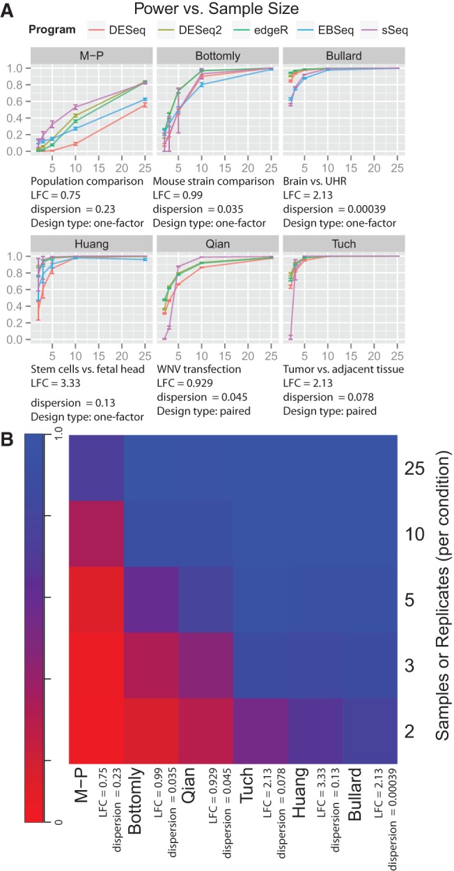
Power curves based on the number of samples per condition for the six public data sets and five RNA-Seq differential expression analysis packages. Library sizes were estimated from the gene counts of the real data sets. Per-gene dispersion was estimated through the Cox–Reid adjusted profile likelihood. (A) Power curves relative to sample size and differential expression methods in six public data sets. The four unpaired-sample data sets (Bottomly, Bullard, Huang, M–P) were analyzed with edgeR, DESeq, DESeq2, EBSeq, and sSeq. The paired-sample data sets (Tuch and Qian) were analyzed with edgeR, DESeq, DESeq2, and sSeq. Note that EBSeq is not included as it is currently not adapted to analyzing paired-sample data. (B) Heatmap of averaged power over the differential expression methods in six public data sets.
Given that power is highly dependent on the data set, we examined the relationships among power, dispersion, and sample size further (Fig. 1; Table 1). Simulations based on the Bullard and Tuch data show that all programs achieve very high power close to one (e.g., 100% detection of DE genes). In the Bullard data set, the estimated median dispersion parameter is extremely low (0.000391). This is likely due to that fact that the samples in this data set are technical replicates rather than biological replicates. Thus all DE analysis packages used here could easily detect differences between the two groups. In the Tuch data, the high power was achieved largely due to the high median FC of DE genes (2.13) (Table 1) and pair-designed samples. On the opposite side, the M–P data consist of transcriptomes from 129 individuals. The M–P data set had the highest median dispersion of 0.231 and the lowest median FC = 0.751 (Table 1). Only DESeq2, edgeR, and sSeq were able to achieve a power of 0.8 or greater at a sample size of 25 samples per condition (Fig. 1).
Performance analysis of other metrics
In addition to statistical power (sensitivity), specificity (complement of FPR) is also an important factor to assess the performance of each DE program. To evaluate them together, we generated receiver operator characteristic (ROC) curves based on the results of the simulated data with 4 samples per condition (Fig. 2A). The most optimal ROC curve jointly displays high levels of TPR and FPR. DESeq2 and edgeR had similar and the best ROC curves for all data sets. DESeq performed similarly to DESeq2 and edgeR, except for the M–P data. However, EBSeq and sSeq generally did not perform as well as the others. EBSeq sometimes yields a large increase in FPR with little corresponding increase in TPR, suggesting its limitation to control the type I error. We also evaluated the different programs with other performance metrics: area under the curve (AUC) of ROC curves, Matthews correlation coefficient (MCC) which takes into account all true and false positives and negatives, and F-measure which is the weighted average of the precision and sensitivity (Fig. 2B). Although we see that no single package consistently performs the worst or the best in all data sets, we did observe similar results as in the ROC curves: DESeq2 and edgeR generally have similar and the best AUC, MCC, and F-measure, except for the M–P data in which sSeq has the best MCC and F-measure (Fig. 2B, Supplemental Figs. S3, S4; Supplemental Table S1). The performance metrics are dependent on the data sets. Generally, data sets with larger dispersions naturally lead to worse accuracy in DE test results, and paired-sample design increases the accuracy of DE test results.
FIGURE 2.

Performance comparison with receiver operator characteristics (ROC) curves and other metrics for the six public data sets and five RNA-Seq differential expression analysis packages. Sensitivity and 1 − specificity were estimated in each simulation for n = 4 samples per condition. The simulations were conducted as in Figure 1. (A) ROC curve comparison. True positive rate (TPR) versus false positive rate (FPR) was plotted. (B) Other performance metrics. Area under the curve (AUC) was measured up to FPR = 0.5 of the ROC curves in A. Matthew correlation coefficient (MCC) and F-measure were measured at the threshold of α = 0.05.
Additionally, we examined the relationship between observed FDR and target FDR in the data sets from the different programs (Supplemental Fig. S5). Similar to the conclusions drawn from the ROC curve metrics, the observed FDRs are dependent on the data sets and programs. Generally, DESeq gives more conservative FDR estimations than others, whereas sSeq tends to give overestimated FDRs.
Improved statistical power by the paired-sample design
In the experimental design, multiple conditions or factors can be set up to affect the expression level of each biological sample. For example, in paired-design experiments, each biological sample has two conditions (such as cancer tissue and cancer adjacent normal tissue) to generate RNA-Seq data. In this study, we used the paired-sample design as a demonstration of multi-factor design, and treated the pairing information as the second factor that affects the expression level of each gene. We used a GLM with negative binomial distribution to estimate the effects of the experimental condition and pairing information, based on parameters estimated from the two paired data sets (Qian and Tuch data). Figure 3 shows the comparisons among the four DE categories in these two data sets, under either single-factor (unpaired) or paired statistical model. It is clear that by considering the pairing information, the statistical power is increased, especially for the Qian data. The Qian data set has a lower median LFC (0.929) relative to the Tuch data set (2.13), as well as a lower median dispersion (∼40% lower than Tuch). This suggests a big advantage to better differentiate genes by introducing additional pairing restrictions, when the overall LFC among genes is not very large. Similar to Figure 1 and regardless of single-factor or paired-sample model, we observed that DESeq2 and edgeR give the highest power estimations when the number of samples is small; however sSeq quickly catches up when the number of samples increases. Again DESeq gives the most conservative estimation of power among the four DE test methods.
FIGURE 3.

Paired versus single-factor power analysis of paired-sample data sets (Qian and Tuch). The data sets were evaluated with pairing information (paired analysis, solid line) or without pairing information (single-factor analysis, dashed line), using the standard analysis pipelines for the respective packages as in Figure 1. Note that EBSeq is not included as it is currently not adapted to analyzing paired-sample data.
Differences in experimental power based on transcript type
Depending on the subsets of transcripts of interest, there might be differences for achievable power. For example, lincRNA are generally expressed at low or medium levels relative to mRNAs from protein coding genes (Cabili et al. 2011; Garmire et al. 2011). Thus the mRNA transcriptome and lincRNA transcriptome may yield different levels of power, even when they are generated from the same RNA-Seq experiments and the same biological samples. To test this, we conducted simulations based on the Huang data set. This data set was chosen because it used ribosomal RNA depletion method rather than poly-A selection, so that lincRNA detection was enhanced. To show the internal difference of the two types of RNAs, we divided the data set by the type of transcripts and summarized the parameters (Table 3). Indeed the most striking difference between the two types of RNAs is the median expression level: The mRNA has a median expression measured in log2 CPM of 4.63, whereas the lincRNA only has a median log2 CPM of 1.25. As expected, the analysis of protein coding genes had higher power compared with the analysis of lincRNA transcripts when the number of samples ≤3, which is often the limit for many experimental laboratories (Fig. 4). DESeq is most conservative in power estimation and showed the largest difference in power between the two types of transcripts, especially when the number of samples is low. At four samples per condition, lincRNAs had a power of 0.65 compared with protein coding genes power of 0.75. However, when the number of samples is sufficient, this difference of power becomes minimal.
TABLE 3.
Estimated parameters of protein-coding genes versus lincRNA transcripts

FIGURE 4.
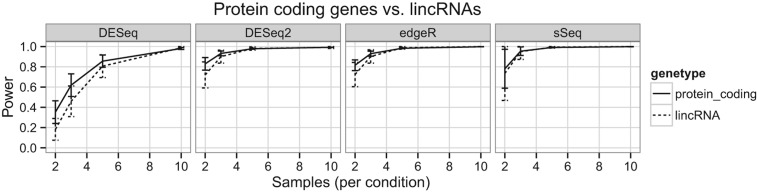
Power of protein coding genes versus long noncoding RNA (lincRNA) transcripts. The comparison was made using the Huang data set, which used ribosomal RNA removal for RNA library construction. The transcriptome was separated into protein coding genes (solid line) or lincRNA (dashed line) categories. Power was estimated in each simulation for these two categories, using the standard analysis pipelines for the respective packages as in Figure 1.
Optimizing sample size and sequencing depth under budget constraints
In real-world RNA-Seq experimental design, the budget constraints usually exist and can significantly affect the trade-off decision between the sample size and sequencing depth. To demonstrate the practical application of RNA-Seq power analysis, we conducted 100 simulations per condition to approximate the optimal sample size and sequencing depth, exemplified by several different budget constraint scenarios ($3000, $5000, $10,000). The cost of RNA-Seq per sample is dependent on the cost of constructing the RNA-Seq library, as well as the cost of sequencing depth (or library size) per sample under the multiplex arrangement, where multiple samples will be barcoded to share one lane of the flow cell. We used an estimated cost of $241 for library construction and $1331 for single-end sequencing cost per lane. Since not all reads map to the transcriptome, we used a mapping percentage of 20%. We determined the optimal power, corresponding sample size, and sequencing depth based on the parameters estimated from the six data sets (Fig. 5 and Supplemental Fig. S6). As demonstrated by the Bottomly data in Figure 5, the higher the budget cap is, the more biological samples are needed (Fig. 5A,C) to reach the optimal power (Fig. 5A,B); however, the sequencing depth does not change much relative to biological samples and stays around 20 million, estimated from most DE methods (Fig. 5D). The highest power was achieved by sSeq, followed closely by DESeq2 and edgeR (Fig. 5A,B). However, sSeq also showed larger standard deviations in the estimated power compared with the other programs (Fig. 5A). DESeq, DESeq2, and edgeR tend to give rise to less skewed power curves across number of samples, relative to EBSeq and sSeq (Fig. 5A). EBSeq tends to yield lower optimal power estimation and skews toward fewer samples but higher sequencing depths, whereas sSeq favors more samples and lower sequencing depth (Fig. 5A,D).
FIGURE 5.

Optimization of power given a budget constraint. The cost of RNA-Seq per sample is dependent on the cost of constructing the RNA-Seq library and the cost of single-end sequencing under the multiplex arrangement, where multiple samples could be barcoded to share one lane of the HiSeq flow cell. Both sequencing depth and sample size are variables under the budget constraint. (A) Power curves relative to samples, exemplified by increasing budgets of $3000, $5000, and $10,000 among five RNA-Seq differential expression analysis packages. (B) Optimal powers achieved for given budget constraints. (C) Biological replicates required to obtain optimal powers for given budget constraints. (D) Sequencing depths required to obtain optimal powers for given budget constraints.
DISCUSSION
RNA-Seq technology is gradually replacing microarray as the method to detect transcriptome level gene expression, therefore it is a critical time to address the problem of desirable statistical power in the RNA-Seq experimental design. There have been a few papers on power and sample size estimation in RNA-Seq experiments; however, these methods need improvement to capture the dispersion in the data and serve as a practical guideline given budget constraints. Busby et al. (2013) measured power as the percentage of genes with twofold count change (by default) that were correctly detected based on the statistical t-test, without realistically capturing the underlying data structure. Hart et al. (2013) performed analysis on 127 RNA-Seq samples in human and fish. They derived a first-order closed form approximation of GLM to compute required sample size and desired power, by taking into account of the variance, expected expression level and fold change. Alternatively, Li et al. (2013) proposed an exact test to replace hyper-geometric probabilities with the negative binomial distribution. However, neither of their methods considered these complexities: (1) more complicated multifactor experimental designs, (2) the various ways to estimate dispersion through different analysis packages (they only used edgeR package), and (3) practical optimization of experimental design given a budget cap. The trade-off between sequencing depth and the number of biological samples was recently studied (Liu et al. 2014). The authors discovered that adding biological samples increases the power to detect DE genes better than the strategy of increasing sequencing depth. However, they did not provide a direct solution for optimization given the fixed budget. Moreover like the others, they did not consider multiple DE analysis packages, multi-factor experimental design, or large scale RNA-Seq experiments such as in the population-based studies.
Compared with these earlier studies, we have made a major leap forward, rather than incremental progress toward providing first-hand and comprehensive references in consideration of RNA-Seq experimental design. We systematically evaluated five popular or more recent DE packages, and conducted simulations based on 212 RNA-Seq samples from six different data sets that span a wide range of experimental conditions, from cell-line, tissue, viral infection, cancer, and population comparisons. We chose the truth data based on more coherent criterion, the intersection of DE genes that are consistent from all different RNA-Seq analysis packages, rather than the more arbitrary LFC threshold like others (Kvam et al. 2012; Robles et al. 2012). Moreover, we provided a reference framework to analyze paired-sample, or more general multifactor experiments, using the GLM approach. Last but not least, we have provided a tool to enable researchers to determine the sample size that optimizes the power, when the budget is limited.
Our study provides many aspects of practical guidance toward the RNA-Seq experimental design. First, dispersion shows a striking impact on power. In data sets with very low dispersions, such as the Bullard data, a power of 0.8 is easily reached with very low sample size and sequencing depth. On the other hand, in data sets with high dispersion, such as M–P data, a power of 0.8 is hardly achievable except at the highest limits of simulation parameters. Due to the strong effect of dispersion, it is clear that statistical tests based on the Poisson distribution (i.e., assuming dispersion = 0) are not capable of handling situations with significant biological variation. Dispersion is primarily due to biological variation; however, it can also be attributed from technical variability such as lane differences and the “shot noise” of the random process (McIntyre et al. 2011). Genes with lower expression have high variance (Anders and Huber 2010), and the subset of DE genes in this group are more likely to have higher fold change (Mutch et al. 2002). All of these factors lead to the challenge of proper estimation of dispersions in the RNA-Seq experiments.
Different RNA-Seq DE testing packages estimate dispersion differently, making the systematical comparisons of these packages worthwhile. We compared the power and other metrics, such as AUC of the ROC curve, MCC and F-measures in five popular or most recent packages. For most data sets, DESeq2 and edgeR give the highest estimate of power, closely followed by DESeq (except the M–P data). DESeq (by default) estimates dispersion by pooling all samples together, fitting them to a parametric distribution and conservatively taking the maximum. This conservative approach may explain why DESeq gives a relatively lower power, as also noted by others (Robles et al. 2012). DESeq2 is the new update to DESeq, and it uses shrinkage estimation for dispersion: The first round of dispersion–mean relationship is obtained by maximum likelihood estimates (MLE), and this fit is then used as a prior to estimate the maximum a posteriori estimate for dispersion in the second round. edgeR estimates dispersion differently. It moderates the dispersion per gene toward a common value across all genes, or toward a local estimate with genes of similar expression. For paired-sample designs, the DESeq package recommends using the Cox–Reid approximate conditional maximum likelihood (CR-APL) method (Anders and Huber 2010). DESeq2 likewise uses the CR-APL method to derive dispersion per gene, and then shrinks the dispersion toward a parametric fit assuming a prior distribution of log dispersion (Wu et al. 2013). edgeR also uses CR-APL and then shrinks the dispersion estimate using empirical Bayes (Robinson et al. 2010). On the other hand, EBseq estimates dispersion by the method of moments, and then uses Bayes posterior probabilities as the measure of statistical significance. While EBSeq generally does not perform as well as other packages, it could outperform others on analyzing isoform level expression (Leng et al. 2013), rather than gene level expression which is the focus of this report. sSeq estimates dispersion by pooling all the samples together using the method of moments, and then shrinking the per-gene estimates through minimizing the mean-square error (Yu et al. 2013). Although the authors of sSeq stated that sSeq compared favorably with other popular packages in low sample sizes regarding sensitivities and specificities, using an external gold standard (Yu et al. 2013), we found that it did not yield the highest powers in the Bottomly and Tuch data sets when the samples are ≤5. This indicates that the performance of sSeq is affected by the data sets or the choice of truth measure.
Two other important factors that influence power are the number of samples and sequencing depth. In general, more biological replicates and greater sequencing depth help to achieve greater statistical power to a certain extent. Sequencing depth is closely related to the expected counts of genes. As sequencing depth increases within the range of 5–20 million reads, genes with lower expression levels, lower fold change and higher dispersions become detectable (Tarazona et al. 2011). However, above 20 million reads, the contribution of sequencing depth to power gain becomes minimal. Combined with preliminary data, sequencing depth can be used for investigating genes of certain expression strengths. For example, if one were interested in estimating the statistical power for lincRNAs, which are on average transcribe 10-fold lower than mRNA transcripts (Cabili et al. 2011), one would not be as concerned about the FDR adjustment for the entire data set. It is therefore possible to enumerate the power and sample size for transcripts of a specific type (e.g., genes with low versus high expression) or over a certain range of parameters (e.g., low LFC versus high LFC). Based on our results, we would recommend a minimum of five samples in order to diminish the power difference between protein coding mRNA and lincRNAs for the sequencing depth of ∼20 million reads.
We also aimed to generalize the potential uses of two-factor analysis by estimating parameters from two paired-sample data sets: The Tuch data set is a paired cancer and normal tissue experiment, and the Qian data set is a paired West Nile Virus and mock transfection of cell cultures. We compared the power to detect DE genes in these two sets using paired analysis versus one-factor analysis, and showed that two-factor models can substantially increase detection limit and hence power in RNA-seq analysis. Furthermore, DESeq, DESeq2, and edgeR are capable of arbitrary design matrices, including scenarios such as time series and blocking design that reduces known variability in confounding factors.
We demonstrated the optimization of RNA-Seq experiments under the budget constraint, a real-world problem for investigators. We showed that a local optimum of power is achievable for a particular samples size. More importantly, we found that the dominant contributing factor to reach optimal power at specific a budget constraint is sample size, rather than sequencing depth which is around the 20 million reads range for most DE detection packages. This conclusion is consistent with Liu et al. (2014), in that biological replicates are more important than read depth for DE detection, although we investigated differently from the power perspective with budget constraints. DESeq, DESeq2, and edgeR presented more symmetrical curves of sample size versus power, whereas EBSeq and sSeq seemed to be more skewed. Correlating to the ROC curves and earlier power estimation without budget constraints, DESeq2 and edgeR appear to be the better choices of software for their overall performances.
As RNA-Seq technology matures and sequencing becomes cheaper, complex experiments with more samples and greater sequencing depth will become more prevalent and there will be an increasing need to design RNA-Seq experiments more thoughtfully. Our approach reported here can be applied more generally to complex multi-factor designs that can be modelled through the GLM framework, such as time series, multi-level designs and blocking designs. We have also demonstrated how optimal sample size and power can be calculated, given a budget constraint. It is our expectation that researchers will find our methods useful and valuable in designing RNA-Seq differential expression experiments.
MATERIALS AND METHODS
Estimation of biological parameters based on real data sets
In this study, we evaluated two different types of experimental designs: paired (two-factor) and unpaired (single-factor) designs. In unpaired experimental designs, samples or individuals in one condition are compared with independent samples in another condition. Paired design is a special case of multifactor (e.g., two-factor, three-factor etc.) designs which consider factors that affect the expression level of each sample. Specifically, in paired experiments each sample has two conditions (such as cancer tissue and cancer adjacent normal tissue) that both yield RNA-Seq data. In this study, we used the paired experimental design as a demonstration of the multifactor design, where the pairing information was treated as the second factor that affects the expression level of each gene.
In our simulated data, we used a general linear model (GLM) with negative binomial distribution. We estimated their parameters from public data sets employed in this study. For the unpaired data sets of two groups, the counts for a particular gene in a sample i were modeled by the following formula:
| (1) |
Here µi is the counts for sample i, Ni is the normalized library size for sample i, β is the vector of coefficients for the two different experimental conditions, and xi is a vector of length two indicating whether sample i belongs to condition one or condition two in the experiment. The LFC was then determined by the difference of the two elements of β. For paired-sample designs, the counts for a gene were modified from equation (1) with the following formula:
| (2) |
Here a new vector of coefficients P of length n/2 is introduced to represent the relative expression level for each pair of samples. The other new vector x2i denotes which pair a particular sample belongs to.
The GLM parameters for each gene in each real data set were estimated by the glm function in R, using a log link function for the count data. The family of negative binomial distributions was calculated by the negative.binomial function in the MASS package. The amount of dispersion per gene was estimated using the Cox–Reid approximate conditional maximum likelihood (CR-APL) method (McCarthy et al. 2012). This method modifies the maximum likelihood estimate of dispersion by accounting for the experimental design through Fisher's Information Matrix in the log-likelihood function (McCarthy et al. 2012). CR-APL is implemented as the dispCoxReidInterpolateTagwise function in the edgeR package, and it is also used in DESeq to estimate the dispersion in multifactor experimental designs.
Generation of simulated count data
The count data were generated from the negative binomial distribution. For each gene, the count Yi was given by
Here, φi is the per-gene dispersion calculated by the CR-APL method, and the expected value μi is a function of the library size. The library size of each simulated sample was generated from a uniform distribution whose parameters were estimated from the maximum and minimum of the real data set.
We used five statistical packages for DE testing: DESeq (version 1.14.0) and edgeR (version 3.4.2) methods, as well as three newer packages released within the past year: DESeq2 (version 1.2.9), EBSeq (version 1.3.1), and sSeq (version 1.0.0). All packages are implemented in the Bioconductor/R platform. We determined the truth data for DE in the simulation as the overlapping DE genes detected from all five statistical packages used in the study, using the original real data sets. This approach is similar to other studies (Rapaport et al. 2013; Soneson and Delorenzi 2013). In the simulation, the LFC of DE genes was determined by equations (1) and (2). We set the LFC of genes that are not differentially expressed to zero in the generation of the simulated count data, as done by others (Soneson and Delorenzi 2013).
Description of public data sets used in the study
The six public data sets are listed in Table 1 (see Results). We enumerate the parameters of each data set in the following.
Bottomly
We used this published data set to compare gene expression between C57BL/6J and DBA/2J mouse strains (Bottomly et al. 2011). An average of 22 million reads was generated for 21 mice (10 C57BL/6J and 11 DBA/2J). Count data were downloaded from the ReCount project (Frazee et al. 2011).
Bullard
Ambion's human brain reference RNA (brain) and Stratagene's Universal Human Reference (UHR) RNA were compared (Bullard et al. 2010). An average of 12.5 million reads was generated from seven brain and seven UHR technical replicates. Count data were also downloaded from ReCount project (Frazee et al. 2011).
Huang
Differentiated embryonic stem cells were compared with fetal head tissues of 14.5 d post coitum. Four biological samples were compared using various rRNA removal methods, in order to analyze coding and noncoding RNAs (Huang et al. 2011). Twenty-two technical replicates were used with an average of 17.7 million reads per sample. Short Read Archive (SRA) reads were downloaded from GEO (GSE22959) and aligned with tophat to mm10 reference genome. Count data were generated using HTSeq (http://www-huber.embl.de/users/anders/HTSeq/doc/overview.html).
Montgomery–Pickrell (M–P)
RNA-seq data from 60 individuals of European descent (Montgomery et al. 2010) and 69 individuals of Nigerian descent (Pickrell et al. 2010) were sequenced with an average sequencing depth of 17 million reads per sample. The data sets were used to analyze DE between the two populations. Count data were downloaded from the ReCount project (Frazee et al. 2011).
Tuch
Three paired tumor and nontumor tissues from oral squamous cell carcinoma patients were sequenced for an average of 205 million reads per sample (Tuch et al. 2010). Count data were downloaded from Supplemental Table S1 of the original publication.
Qian
West Nile Virus (WNV) transfection of macrophage cells from 10 healthy donors were compared with mock transfection of the same cell culture with a total of 28 million reads per sample (Qian et al. 2013). Raw SRA read data were downloaded from GEO (GSE40718) and aligned with tophat to Hg19 Refseq genes downloaded from UCSC Genome Browser. Count data were also generated using HTSeq.
Detection of DE in unpaired (single-factor) experimental designs
We aimed to calculate P-values, sensitivity (power) and specificity over the range of parameters. Toward these aims, we performed standard analyses with functions implemented in the five RNA-Seq analysis packages DESeq2, DESeq, edgeR, sSeq, and EBSeq. Specifically, in DESeq the count data were analyzed using newCountDataSet, followed by estimateSizeFactors, estimateDispersions, and nbinomTest functions. For DESeq2, DESeqDataSetFromMatrix was used, followed by estimateSizeFactors, estimateDispersions, and nbinomWald Test functions. For edgeR, count data were analyzed using DGEList followed by calcNormFactors, estimateCommonDisp, estimate TagwiseDisp, and exactTest functions. For EBSeq, the libraries were first normalized using MedianNorm and then DE genes were detected using the EBTest function. For sSeq, DE genes were detected using nbTestSH function. In packages where P-value adjustment was needed, the p.adjust function in R with method=“BH” (Benjamini and Hochberg FDR option) was employed.
Detection of DE in paired-sample (two-factor) experimental designs
Similar to the unpaired or single-factor designs, we performed standard analyses for the paired-sample experimental designs. We calculated P-values, sensitivity (power) and specificity over the range of parameters, using four statistical packages: DESeq2, DESeq, edgeR, and sSeq. We did not conduct DE gene detection using EBSeq, as it is not adapted to analyzing paired data currently (C Kendziorski, Y Li, and N Leng, pers. comm.). In DESeq, data were analyzed similar to above, using the two-factor design matrix and “method=pooled-CR” for the dispersion estimation, followed by fitNbinomGLMs function for both the null and alternative hypotheses, and then by nbinomGLMTest function to calculate P-values per gene. DESeq2 was used similarly to the single-factor analysis above, using the two-factor design matrix (condition + pairing information). For edgeR, count data were analyzed using DGEList followed by calcNormFactors, estimateCommonDisp, estimateGLMTrendedDisp, estimateTagwiseDisp, glmFit, and glmLRT functions. For sSeq, function nbTestSH was used with pairedDesign=TRUE and coLevels= the pairing information. P-value adjustment was done the same way as in single-factor design, when needed.
Calculation of true positive rates (power) and false positive rates
The sample sizes in the simulated data sets varied from n = 2 to n = 25 and the average library sizes varied from 1 million up to 50 million reads. Each condition was simulated 100 times using random seeds 1 to 100 using the set.seed function in R. Given a significance threshold of 0.05, the TPR was calculated by
 |
and the FPR was calculated by
 |
Two standard performance measures, Matthews correlation coefficient (MCC, also known as the ϕ statistic) and F-measure are calculated by
 |
and
 |
where TP is true positives, TN is true negatives, FP is false positives, and FN is false negatives.
Planning RNA-Seq under the budget constraint
For RNA-Seq cost calculation, we referred to Illumina Hi-Seq single-end RNA-Seq prices listed by the Yale Center for Genome Analysis (http://ycga.yale.edu/services/illuminaprices.aspx). The total overhead cost of each sample was estimated as $241, which includes sample quality check and mRNA library construction. The remaining sequencing cost per lane was $1331 based on HiSeq 2000 single-end sequencing. Simulated count data were generated as before, by modeling gene counts through equation (1) or (2) and the negative binomial distribution. The formula to calculate the budget is as follows:
 |
All R code is available for downloading from our website: http://www2.hawaii.edu/~lgarmire/RNASeqPowerCalculator.htm
SUPPLEMENTAL MATERIAL
Supplemental material is available for this article.
Supplementary Material
ACKNOWLEDGMENTS
We thank Dr. Lynne Wilkens for reviewing the manuscript, and Dr. Christina Kendziorski and her students for the communications in using EBSeq. We thank Dr. Gordon Okimoto and Mr. Mike Loomis for providing access to the server clusters of Biostatistics and Bioinformatics Shared Resources at University of Hawaii Cancer Center. This work was supported by the National Institute of General Medical Sciences (P20 COBRE GM103457).
Footnotes
Article published online ahead of print. Article and publication date are at http://www.rnajournal.org/cgi/doi/10.1261/rna.046011.114.
REFERENCES
- Aban IB, Cutter GR, Mavinga N. 2008. Inferences and power analysis concerning two negative binomial distributions with an application to MRI lesion counts data. Comput Stat Data Anal 53: 820–833 [DOI] [PMC free article] [PubMed] [Google Scholar]
- Anders S, Huber W. 2010. Differential expression analysis for sequence count data. Genome Biol 11: R106. [DOI] [PMC free article] [PubMed] [Google Scholar]
- Bottomly D, Walter NA, Hunter JE, Darakjian P, Kawane S, Buck KJ, Searles RP, Mooney M, McWeeney SK, Hitzemann R. 2011. Evaluating gene expression in C57BL/6J and DBA/2J mouse striatum using RNA-Seq and microarrays. PLoS One 6: e17820. [DOI] [PMC free article] [PubMed] [Google Scholar]
- Bullard JH, Purdom E, Hansen KD, Dudoit S. 2010. Evaluation of statistical methods for normalization and differential expression in mRNA-Seq experiments. BMC Bioinformatics 11: 94. [DOI] [PMC free article] [PubMed] [Google Scholar]
- Busby MA, Stewart C, Miller CA, Grzeda KR, Marth GT. 2013. Scotty: a web tool for designing RNA-Seq experiments to measure differential gene expression. Bioinformatics 29: 656–657 [DOI] [PMC free article] [PubMed] [Google Scholar]
- Cabili MN, Trapnell C, Goff L, Koziol M, Tazon-Vega B, Regev A, Rinn JL. 2011. Integrative annotation of human large intergenic noncoding RNAs reveals global properties and specific subclasses. Genes Dev 25: 1915–1927 [DOI] [PMC free article] [PubMed] [Google Scholar]
- Chen Z, Liu J, Ng HKT, Nadarajah S, Kaufman HL, Yang JY, Deng Y. 2011. Statistical methods on detecting differentially expressed genes for RNA-seq data. BMC Syst Biol 5(Suppl 3): S1. [DOI] [PMC free article] [PubMed] [Google Scholar]
- Frazee A, Langmead B, Leek J. 2011. ReCount: a multi-experiment resource of analysis-ready RNA-seq gene count datasets. BMC Bioinformatics 12: 449. [DOI] [PMC free article] [PubMed] [Google Scholar]
- Garmire LX, Garmire DG, Huang W, Yao J, Glass CK, Subramaniam S. 2011. A global clustering algorithm to identify long intergenic non-coding RNA—with applications in mouse macrophages. PLoS One 6: e24051. [DOI] [PMC free article] [PubMed] [Google Scholar]
- Hart SN, Therneau TM, Zhang Y, Poland GA, Kocher J-P. 2013. Calculating sample size estimates for RNA sequencing data. J Comput Biol 20: 970–978 [DOI] [PMC free article] [PubMed] [Google Scholar]
- Huang R, Jaritz M, Guenzl P, Vlatkovic I, Sommer A, Tamir IM, Marks H, Klampfl T, Kralovics R, Stunnenberg HG. 2011. An RNA-Seq strategy to detect the complete coding and non-coding transcriptome including full-length imprinted macro ncRNAs. PLoS One 6: e27288. [DOI] [PMC free article] [PubMed] [Google Scholar]
- Jiang H, Wong WH. 2009. Statistical inferences for isoform expression in RNA-Seq. Bioinformatics 25: 1026–1032 [DOI] [PMC free article] [PubMed] [Google Scholar]
- Kim D, Salzberg SL. 2011. TopHat-Fusion: an algorithm for discovery of novel fusion transcripts. Genome Biol 12: R72. [DOI] [PMC free article] [PubMed] [Google Scholar]
- Kvam VM, Liu P, Si Y. 2012. A comparison of statistical methods for detecting differentially expressed genes from RNA-seq data. Am J Bot 99: 248–256 [DOI] [PubMed] [Google Scholar]
- Leng N, Dawson JA, Thomson JA, Ruotti V, Rissman AI, Smits BM, Haag JD, Gould MN, Stewart RM, Kendziorski C. 2013. EBSeq: an empirical Bayes hierarchical model for inference in RNA-seq experiments. Bioinformatics 29: 1035–1043 [DOI] [PMC free article] [PubMed] [Google Scholar]
- Li CI, Su PF, Shyr Y. 2013. Sample size calculation based on exact test for assessing differential expression analysis in RNA-seq data. BMC Bioinformatics 14: 357. [DOI] [PMC free article] [PubMed] [Google Scholar]
- Liu Y, Zhou J, White KP. 2014. RNA-seq differential expression studies: more sequence or more replication? Bioinformatics 30: 301–304 [DOI] [PMC free article] [PubMed] [Google Scholar]
- Love MI, Huber W, Anders S. 2014. Moderated estimation of fold change and dispersion for RNA-Seq data with DESeq2. bioRxiv 10.1101/002832 [DOI] [PMC free article] [PubMed] [Google Scholar]
- Marioni JC, Mason CE, Mane SM, Stephens M, Gilad Y. 2008. RNA-seq: an assessment of technical reproducibility and comparison with gene expression arrays. Genome Res 18: 1509–1517 [DOI] [PMC free article] [PubMed] [Google Scholar]
- McCarthy DJ, Chen Y, Smyth GK. 2012. Differential expression analysis of multifactor RNA-Seq experiments with respect to biological variation. Nucleic Acids Res 40: 4288–4297 [DOI] [PMC free article] [PubMed] [Google Scholar]
- McCulloch CE. 1997. Maximum likelihood algorithms for generalized linear mixed models. J Am Stat Assoc 92: 162–170 [Google Scholar]
- McIntyre LM, Lopiano KK, Morse AM, Amin V, Oberg AL, Young LJ, Nuzhdin SV. 2011. RNA-seq: technical variability and sampling. BMC Genomics 12: 293. [DOI] [PMC free article] [PubMed] [Google Scholar]
- Montgomery SB, Sammeth M, Gutierrez-Arcelus M, Lach RP, Ingle C, Nisbett J, Guigo R, Dermitzakis ET. 2010. Transcriptome genetics using second generation sequencing in a Caucasian population. Nature 464: 773–777 [DOI] [PMC free article] [PubMed] [Google Scholar]
- Morin RD, Bainbridge M, Fejes A, Hirst M, Krzywinski M, Pugh TJ, McDonald H, Varhol R, Jones SJM, Marra MA. 2008. Profiling the HeLa S3 transcriptome using randomly primed cDNA and massively parallel short-read sequencing. Biotechniques 45: 81–94 [DOI] [PubMed] [Google Scholar]
- Mutch DM, Berger A, Mansourian R, Rytz A, Roberts M-A. 2002. The limit fold change model: a practical approach for selecting differentially expressed genes from microarray data. BMC Bioinformatics 3: 17. [DOI] [PMC free article] [PubMed] [Google Scholar]
- Nookaew I, Papini M, Pornputtapong N, Scalcinati G, Fagerberg L, Uhlén M, Nielsen J. 2012. A comprehensive comparison of RNA-Seq-based transcriptome analysis from reads to differential gene expression and cross-comparison with microarrays: a case study in Saccharomyces cerevisiae. Nucleic Acids Res 40: 10084–10097 [DOI] [PMC free article] [PubMed] [Google Scholar]
- Pham TV, Jimenez CR. 2012. An accurate paired sample test for count data. Bioinformatics 28: i596–i602 [DOI] [PMC free article] [PubMed] [Google Scholar]
- Pickrell JK, Marioni JC, Pai AA, Degner JF, Engelhardt BE, Nkadori E, Veyrieras J-B, Stephens M, Gilad Y, Pritchard JK. 2010. Understanding mechanisms underlying human gene expression variation with RNA sequencing. Nature 464: 768–772 [DOI] [PMC free article] [PubMed] [Google Scholar]
- Qian F, Chung L, Zheng W, Bruno V, Alexander RP, Wang Z, Wang X, Kurscheid S, Zhao H, Fikrig E, et al. 2013. Identification of genes critical for resistance to infection by West Nile virus using RNA-Seq analysis. Viruses 5: 1664–1681 [DOI] [PMC free article] [PubMed] [Google Scholar]
- Rapaport F, Khanin R, Liang Y, Pirun M, Krek A, Zumbo P, Mason CE, Socci ND, Betel D. 2013. Comprehensive evaluation of differential gene expression analysis methods for RNA-seq data. Genome Biol 14: R95. [DOI] [PMC free article] [PubMed] [Google Scholar]
- Rau A, Gallopin M, Celeux G, Jaffrezic F. 2013. Data-based filtering for replicated high-throughput transcriptome sequencing experiments. Bioinformatics 29: 2146–2152 [DOI] [PMC free article] [PubMed] [Google Scholar]
- Robinson MD, Oshlack A. 2010. A scaling normalization method for differential expression analysis of RNA-seq data. Genome Biol 11: R25. [DOI] [PMC free article] [PubMed] [Google Scholar]
- Robinson MD, Smyth GK. 2007. Moderated statistical tests for assessing differences in tag abundance. Bioinformatics 23: 2881–2887 [DOI] [PubMed] [Google Scholar]
- Robinson MD, McCarthy DJ, Smyth GK. 2010. edgeR: a Bioconductor package for differential expression analysis of digital gene expression data. Bioinformatics 26: 139–140 [DOI] [PMC free article] [PubMed] [Google Scholar]
- Robles JA, Qureshi SE, Stephen SJ, Wilson SR, Burden CJ, Taylor JM. 2012. Efficient experimental design and analysis strategies for the detection of differential expression using RNA-Sequencing. BMC Genomics 13: 484. [DOI] [PMC free article] [PubMed] [Google Scholar]
- Soneson C, Delorenzi M. 2013. A comparison of methods for differential expression analysis of RNA-seq data. BMC Bioinformatics 14: 91. [DOI] [PMC free article] [PubMed] [Google Scholar]
- Srivastava S, Chen L. 2010. A two-parameter generalized Poisson model to improve the analysis of RNA-seq data. Nucleic Acids Res 38: e170. [DOI] [PMC free article] [PubMed] [Google Scholar]
- Tarazona S, García-Alcalde F, Dopazo J, Ferrer A, Conesa A. 2011. Differential expression in RNA-seq: a matter of depth. Genome Res 21: 2213–2223 [DOI] [PMC free article] [PubMed] [Google Scholar]
- Trapnell C, Pachter L, Salzberg SL. 2009. TopHat: discovering splice junctions with RNA-Seq. Bioinformatics 25: 1105–1111 [DOI] [PMC free article] [PubMed] [Google Scholar]
- Tuch BB, Laborde RR, Xu X, Gu J, Chung CB, Monighetti CK, Stanley SJ, Olsen KD, Kasperbauer JL, Moore EJ. 2010. Tumor transcriptome sequencing reveals allelic expression imbalances associated with copy number alterations. PLoS One 5: e9317. [DOI] [PMC free article] [PubMed] [Google Scholar]
- Vijay N, Poelstra JW, Künstner A, Wolf JBW. 2013. Challenges and strategies in transcriptome assembly and differential gene expression quantification. A comprehensive in silico assessment of RNA-seq experiments. Mol Ecol 22: 620–634 [DOI] [PubMed] [Google Scholar]
- Wang Z, Gerstein M, Snyder M. 2009. RNA-Seq: a revolutionary tool for transcriptomics. Nat Rev Genet 10: 57–63 [DOI] [PMC free article] [PubMed] [Google Scholar]
- Wang L, Feng Z, Wang X, Wang X, Zhang X. 2010. DEGseq: an R package for identifying differentially expressed genes from RNA-seq data. Bioinformatics 26: 136–138 [DOI] [PubMed] [Google Scholar]
- Wu H, Wang C, Wu Z. 2013. A new shrinkage estimator for dispersion improves differential expression detection in RNA-seq data. Biostatistics 14: 232–243 [DOI] [PMC free article] [PubMed] [Google Scholar]
- Yu D, Huber W, Vitek O. 2013. Shrinkage estimation of dispersion in Negative Binomial models for RNA-seq experiments with small sample size. Bioinformatics 29: 1275–1282 [DOI] [PMC free article] [PubMed] [Google Scholar]
Associated Data
This section collects any data citations, data availability statements, or supplementary materials included in this article.