Diffusion of Fiber Orientation Distribution Functions with a Rotation-Induced Riemannian Metric

Abstract

Advanced diffusion weighted MR imaging allows non-invasive study on the structural connectivity of human brains. Fiber orientation distributions (FODs) reconstructed from diffusion data are a popular model to represent crossing fibers. For this sophisticated image representation of connectivity, classical image operations such as smoothing must be redefined. In this paper, we propose a novel rotation-induced Riemannian metric for FODs, and introduce a weighted diffusion process for FODs regarding this Riemannian manifold. We show how this Riemannian manifold can be used for smoothing, interpolation and building image-pyramids, yielding more accurate or intuitively more reasonable results than the linear or the unit hyper-sphere manifold.

1 Introduction

The Human Connectome Project [1] has provided cutting-edge diffusion MR imaging techniques to study brain anatomical connectivity in vivo at unprecedented spatial and angular resolution. This advancement urges the development of novel mathematical methods to modelling neural fibers.

Fiber orientation distribution (FOD) images, reconstructed from diffusion weighted images, are widely used to represent the spatial and orientational distribution of neural fibers. At each voxel location p, the likelihood of fibers along a direction u is described by a real-valued and nonnegative function F(u).

The mathematical property of FODs is more complicated than that of intensity values or diffusion tensors, so their fundamental operations such as smoothing and interpolation cannot be conducted in the same way. For example, linear smoothing does not yield satisfactory results, as shown in Section 5.2. In [2,3,4], $f=\sqrt{F}$ is modeled as a point on the unit hyper-sphere, a manifold whose exponential and logarithmic maps are well studied. Later in [5,6], FODs are separated as two parts: orientation and shape. FODs’ comparison and interpolation are conducted by rotationally matching their shapes.

In this paper, we propose a rotation-induced Riemannian metric for square-rooted FODs f, and introduce a weighted diffusion process for FODs regarding this metric. This novel weighted diffusion process can be used for smoothing, interpolation and down-sampling of FOD images. It may potentially benefit many down-stream tasks, such as tractography or registration. It can also be used to build FOD image pyramids for multi-scale image processing. Contrast to the work in [5,6], we focus on the differential structure of FODs, instead of their weighted average. In an experiment with real images, we compared the new method with the linear manifold and the hyper-sphere manifold. The new method keeps fiber integrity better in smoothing and down-sampling, and yields more accurate results in interpolation.

2 Rotation and Spherical Functions

2.1 Rotation and Angular Velocity

Any rotation in can be described with a rotation vector r⃗ = [r_x,r_y,r_z] (||r⃗|| ≤ π) whose direction r⃗ / ||r⃗|| is the pivot axis according to the right-hand rule and whose length ||r⃗|| is the rotation angle. The rotation matrix associated with r⃗ is R = e^[r⃗]× where [•]^× is the cross-product matrix of a 3D vector as define in Eq. (1),

$${[•]}^{\times }\equiv \left[\begin{array}{ccc}0& -{•}_z& {•}_y\\ {•}_z& 0& -{•}_x\\ -{•}_y& {•}_x& 0\end{array}\right].$$ (1)

An angular velocity vector ω⃗ describes the pivot axis and spinning speed of a rotating object respectively with its direction and amplitude. If an object spinning with ω⃗ for time duration t, the accumulated rotation effect, parameterized as a rotation matrix, is R = e^t[ω⃗]×. With R, a point p ∈ rotates to Rp.

2.2 Rotation of Spherical Functions

If a spherical function f(u) is rotated with R, it becomes f(R⁻¹u). Given a unit angular velocity ω⃗ (||ω⃗|| = 1), we define

$${\stackrel{.}{f}}_{\overrightarrow{\omega }}(u)\equiv \frac{d}{dt}{\mid }_{t=0}f(e^{-t{[\overrightarrow{\omega }]}^{\times }}u)$$ (2)

as the rotation differential of f around axis ω⃗.

3 Manifolds of FODs

An FOD F is a spherical probability density function satisfies both ∫_u∈S² F(u)du = 1 and F(u) ≥ 0, where S² is a unit sphere in . Cheng, etc. in [2] modelled the manifold $M\equiv \{f(u)=\sqrt{F(u)}\}$ as a unit hyper-sphere, assuming that f can be linearly represented by a finite number of orthonormal base functions. In this section, we propose a Riemannian metric for M, differently weighting the effect of rotation in . For simplicity, symbols such as “f”, “v” or “l”, depending on the context, denote either spherical functions, or their linear coordinates as represented by orthonormal base functions.

3.1 Hyper-Sphere

For two spherical functions f₁ and f₂, we define 〈f₁, f₂〉 ≡ ∫_u∈S² f₁(u)f₂(u)du as their dot product. As any f ∈ M satisfies 〈f, f〉 = 1, M is a unit hyper-sphere, a well-studied Riemannian manifold. Given a point f ∈ M, another point f^† ∈ M near f can be logarithmically mapped to T_fM, the tangent space at f, as

$${log}_f(f^{†})=v_f=\frac{f^{†}-fcos\phi }{\Vert f^{†}-fcos\phi \Vert }\phi ,\text{where}\phi =arccos(\langle f,f^{†}\rangle )$$ (3)

The Riemannian metric at f associated with the logarithmic map is g_f(v₁, v₂) = 〈v₁, v₂〉 where v₁, v₂ ∈ T_fM are two tangent vectors at f.

3.2 Rotation-Induced Riemannian Metric

Riemannian metric g_f is isotropic, treating all the directions in T_fM equally. To incorporate rotation into the metric, tangent vectors generated by rotating f in should be treated differently. Let ḟ_x, ḟ_y and ḟ_z denote the rotation differential of f respectively around the x, y, and z axes, as defined in Eq. (2). As ḟ_x, ḟ_y and ḟ_z are in T_fM, we use them to induce a Riemannian metric as follows. First, for a tangent vector v, we project it to the subspace spanned by ḟ_x, ḟ_y and ḟ_z. Let c_xḟ_x + c_yḟ_y + c_zḟ_z be the projection, c ≡ [c_x, c_y, c_z] the projection coefficients, and ξ ≡ v − c_xḟ_x + c_yḟ_y + c_zḟ_z the residual. Second, given two tangent vectors v₁ and v₂, the induced Riemannian metric is defined as

$$g_f^{\ast }(v_1,v_2)=\lambda \langle c_1,c_2\rangle +\langle {\xi }_1,{\xi }_2\rangle$$

where λ > 0 is a parameter weighting the contribution of rotation. Such a metric definition is equivalent to $g_f^{\ast }(v_1,v_2)=\langle v_1^{\ast },v_2^{\ast }\rangle$ where $v_{•}^{\ast }=G_f{v}_{•}$ and G_f is a full-rank transformation matrix induced by ḟ_x, ḟ_y, ḟ_z and λ. The g_f in Section 3.1 can be regarded as using G_f = I.

As ḟ_x, ḟ_y and ḟ_z are not necessarily linearly independent, the projection coefficients c may not be unique. To resolve the ambiguity, we choose the coefficients with the least norm. Let b₁, …, b_m be a set of unitary bases of the subspace spanned by ḟ_x, ḟ_y and ḟ_z. The least norm projection coefficients are

$$c=A^T{({AA}^T)}^{-1}\left[\begin{array}{c}\langle b_1,v\rangle \\ ⋮\\ \langle b_m,v\rangle \end{array}\right]\text{where}A=\left[\begin{array}{ccc}\langle b_1,{\stackrel{.}{f}}_x\rangle & \langle b_1,{\stackrel{.}{f}}_y\rangle & \langle b_1,{\stackrel{.}{f}}_z\rangle \\ ⋮& ⋮& ⋮\\ \langle b_m,{\stackrel{.}{f}}_x\rangle & \langle b_m,{\stackrel{.}{f}}_y\rangle & \langle b_m,{\stackrel{.}{f}}_z\rangle \end{array}\right].$$

The Riemannian metric $g_f^{\ast }$ introduces a new logarithmic map near f. The length of a smooth curve γ: [0, 1] → M is $L^{\ast }(\gamma )={\int }_0^1\sqrt{g_{\gamma }^{\ast }[{\gamma }^{\prime }(t),{\gamma }^{\prime }(t)]}dt$. The geodesic from f to a nearby point f^† is a curve γ which satisfies γ(0) = f and γ(1) = f^† and minimizes L*(γ). With appropriate re-parameterization of t, $g_{\gamma }^{\ast }[{\gamma }^{\prime }(t),{\gamma }^{\prime }(t)]$ can be time-invariant. Accordingly, the logarithmic map of f^† to T_fM is ${log}_f^{\ast }(f^{†})=G_f{\gamma }^{\prime }(0)$.

4 Weighted Diffusion of FODs

An FOD image is a mapping from to an FOD manifold M. Given a point p in , let f_p denote its square-rooted FOD. To calculate the diffusion force at p, we construct a local helper function h_p: h_p(q) ≡ LOG_fp(f_q) where q is a point near p and h_p(q) is the logarithmic map of f_q to T_fpM. It should be noted that the definition of LOG_fp is subject to the definition of Riemannian metrics. Sections 3.1 and 3.2 describes different metrics and logarithmic maps.

A weighted diffusion process on an FOD image is

$$\frac{{df}_p}{dt}=\frac{1}{w_p}{l}_p\equiv \frac{1}{w_p}{G}_{f_p}^{-1}\left(\frac{{\partial }^2{h}_p}{\partial x^2}+\frac{{\partial }^2{h}_p}{\partial y^2}+\frac{{\partial }^2{h}_p}{\partial z^2}\right)$$ (4)

where l_p is the diffusion force at point p, and w_p is a positive weight associated with point p in the FOD image. $G_{f_p}^{-1}$ maps the diffusion force to tangent space of the hyper-sphere manifold. FODs at points with higher weights changes slower than those with lower weights. We assume that such a diffusion process eventually makes every point in the image take the same FOD value.

The weighed diffusion can be applied to FOD image processing as follows:

• Smoothing: diffusion in .

• Interpolation: weighted diffusion within a 2×2×2 voxel cube.

• Down-Sampling: diffusion followed by interpolation.

5 Evaluation

We compare three different manifold models of FODs: the linear model, the unit hyper-sphere model, and the rotation-induced manifold. For simplicity, we call them the linear, the hSphere and the rSphere methods. With the three models, image processing tasks smoothing, interpolation and down-sampling are conducted on real FOD images. Their performances are evaluated with two indices: (1) the sharpness of their output FODs and (2) the difference from baseline images depending on the processing tasks. The sharpness of FODs is measured with the generalized Fractional Anisotropy gFA(f) = 2dist(f₀, f)/π where f₀ is the uniform spherical function in M, and dist(•, •) ≡ arccos(〈•,•〉); the difference from a baseline is measured with δ(f) = 2dist(f_b, f)/π where f_b is the baseline FOD. (The factor 2/π scales the indices into range [0, 1].)

Pixel-wise comparison within each subject is conducted as follows: a performance index image of one method is subtracted from that of another method, and then the histogram of the subtracted image is plotted. The subject-wise comparison is conducted as follows: for every subject, a voxel-averaged performance index is calculated, and the averaged indices of subjects are compared with the t-test between the three methods.

5.1 Data

Ten subjects are randomly selected from the Human Connectome Project. The diffusion data were acquired with a multi-shell sampling scheme, and the FOD images, represented with the 8-th order spherical harmonics [7], were reconstructed with the method in [8].

5.2 Smoothing

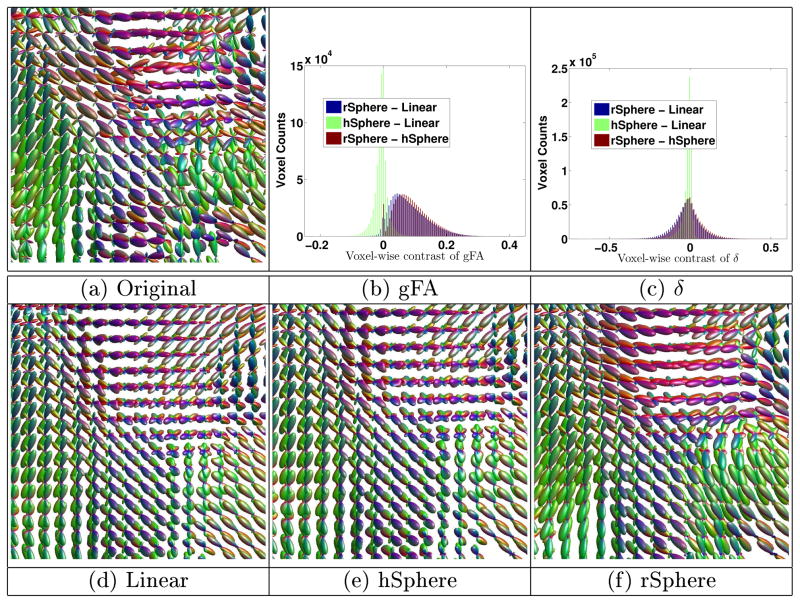
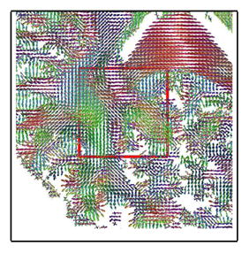
Images are diffused with time duration t = 1. gFA is calculated on the diffused images, and the original images are the baseline images of δ. The diffused images of a subject is shown in Figure 1, taken from the highlighted region in the figure besides Table 1. The rSphere method yields more reasonable results, as the fibers are sharper and orientationally smoother. The linear and hSphere methods yield “bloated” FODs. Figures 1(b) and 1(c) show the histogram of the pixel-wise contrast of the gFA and δ indices among the three methods. The rSphere method produces higher gFA than the other two methods. Table 1 shows the t-test of subject-wise comparison. The rSphere method makes slightly less changes (low δ) from the original images, yet keeps the diffused FODs much sharper (high gFA). Tiny p-values evidence the statistical significance of the results.

Fig. 1.

Example of smoothing. The rSphere method produces sharper and orientationally smoother FODs. The linear and the hSphere methods produce “bloated” FODs.

Table 1.

Subject-wise comparison of smoothing.

	gFA		δ
	mean	p-value	mean	p-value
rS. - hS.	0.092 ± 0.002	8.14e-16	−0.0059 ± 0.0011	6.54e-7
rS. - L.	0.084 ± 0.002	2.02e-15	−0.0221 ± 0.0013	2.22e-11
hS. - L.	−0.007 ± 0.003	1.51e-12	−0.0162 ± 0.0004	3.33e-15

5.3 Interpolation

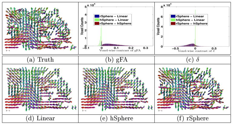
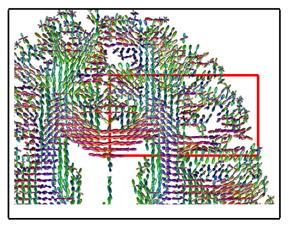
Images are sub-sampled into two parts: one of odd-index voxels and the other of even-index. FODs at even-index voxels are then interpolated from the odd-index image, and then compared with the original even-index image. gFA is calculated on the interpolated images, and the original even-index images are the baseline images of δ. The interpolation results of a subject is shown in Figure 2, taken from the highlighted region in the figure besides Table 2. The rSphere method yields more accurate results, with FODs more similar to the original image. Figures 2(b) and 2(c) show the histogram of the pixel-wise contrast of the gFA and δ indices among the three methods. The rSphere method yields higher gFA and lower δ than the other two methods. Table 2 shows the t-test of subject-wise comparison. The rSphere outperforms the other two methods with higher gFA and lower δ. Tiny p-values evidence the statistical significance of the results.

Fig. 2.

Example of interpolation. The rSphere results are more similar to the truth.

Table 2.

Subject-wise comparison of interpolation.

	gFA		δ
	mean	p-value	mean	p-value
rS. - hS.	+0.071 ± 0.0015	3.35e-15	−0.131 ± 0.0034	1.72e-14
rS. - L.	+0.064 ± 0.0015	6.87e-15	−0.134 ± 0.0035	1.95e-14
hS. - L.	−0.0061 ± 0.0002	2.60e-13	−0.0033 ± 0.0005	2.45e-07

5.4 Down-Sampling

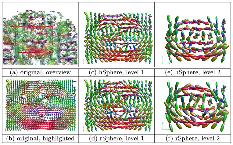
Down-sampling is conducted as follows. Images are diffused with time duration t = 1 and then is interpolated for the down-sampled voxel locations. Two-level down-sampling is conducted to build image pyramids. gFA is calculated on the down-sampled images. The down-sampled results of a subject is shown in Figure 3. Sub-figures (a) and (b) show respectively the overview and highlighted region of the original image. Sub-figures (c) and (e) show the down-sampled images of the hSphere method, sub-figures (d) and (f) show those of the rSphere method. (Due to limited page room, the following contents are not presented here: the results of linear down-sampling which are very similar to the hSphere method, the histogram of pixel-wise contrast of the gFA index which is very similar to the smoothing and interpolation tasks.) The rSphere produces sharper FODs. Table 3 shows the t-test of subject-wise comparison of gFA. The rSphere yields higher gFA, indicating the down-sampled FODs are shaper than the other methods. Tiny p-values evidence the statistical significance of the results.

Fig. 3.

Example of down-sampling. The rSphere method produces sharper FODs.

Table 3.

Subject-wise comparison of down-sampling, regarding the gFA index.

	Level-1		Level-2
	mean	p-value	mean	p-value
rSphere - hSphere	+0.035 ± 0.0008	3.43e-15	0.082 ± 0.0012	8.03e-17
rSphere - Linear	+0.033 ± 0.0008	2.85e-15	0.075 ± 0.0011	7.82e-17
hSphere - Linear	−0.0015 ± 0.0001	1.24e-13	−0.0077 ± 0.0002	4.30e-15

6 Conclusion

Weighted diffusion of square-rooted FODs f with the rotation-induced Riemannian metric leads to significantly better smoothing, interpolation and down-sampling of FOD images, in comparison with the linear manifold, and the hyper-sphere manifold.

References

- 1.Human Connectome Project. http://www.humanconnectomeproject.org/
- 2.Cheng Jian, Ghosh Aurobrata, Jiang Tianzi, Deriche Rachid. A Riemannian framework for orientation distribution function computing. Medical Image Computing and Computer-Assisted Intervention–MICCAI; 2009; Springer; 2009. pp. 911–918. [DOI] [PubMed] [Google Scholar]
- 3.Du Jia, Goh Alvina, Qiu Anqi. Diffeomorphic metric mapping of high angular resolution diffusion imaging based on Riemannian structure of orientation distribution functions. Medical Imaging, IEEE Transactions on. 2012;31(5):1021–1033. doi: 10.1109/TMI.2011.2178253. [DOI] [PubMed] [Google Scholar]
- 4.Srivastava Anuj, Jermyn Ian, Joshi Shantanu. Riemannian analysis of probability density functions with applications in vision. Computer Vision and Pattern Recognition, 2007. CVPR’07. IEEE Conference; IEEE; 2007. pp. 1–8. [DOI] [PMC free article] [PubMed] [Google Scholar]
- 5.Ncube Sentibaleng, Srivastava Anuj. A novel Riemannian metric for analyzing HARDI data. SPIE Medical Imaging; International Society for Optics and Photonics; 2011. pp. 79620Q–79620Q. [Google Scholar]
- 6.Cetingul Hasan Ertan, Afsari Bijan, Wright Margaret J, Thompson Paul M, Vidal René. Group action induced averaging for HARDI processing. Biomedical Imaging (ISBI), 2012 9th IEEE International Symposium; IEEE; 2012. pp. 1389–1392. [DOI] [PMC free article] [PubMed] [Google Scholar]
- 7.Hill David A. Electromagnetic Fields in Cavities: Deterministic and Statistical Theories. Wiley-IEEE Press; 2009. [Google Scholar]
- 8.Tran Giang, Shi Yonggang. Adaptively constrained convex optimization for accurate fiber orientation estimation with high order spherical harmonics. Medical Image Computing and Computer-Assisted Intervention–MICCAI; 2013; 2013. pp. 485–492. [DOI] [PMC free article] [PubMed] [Google Scholar]