A Comprehensive Comparison of Normalization Methods for Loading Control and Variance Stabilization of Reverse-Phase Protein Array Data

Abstract

Loading control (LC) and variance stabilization of reverse-phase protein array (RPPA) data have been challenging mainly due to the small number of proteins in an experiment and the lack of reliable inherent control markers. In this study, we compare eight different normalization methods for LC and variance stabilization. The invariant marker set concept was first applied to the normalization of high-throughput gene expression data. A set of “invariant” markers are selected to create a virtual reference sample. Then all the samples are normalized to the virtual reference. We propose a variant of this method in the context of RPPA data normalization and compare it with seven other normalization methods previously reported in the literature. The invariant marker set method performs well with respect to LC, variance stabilization and association with the immunohistochemistry/florescence in situ hybridization data for three key markers in breast tumor samples, while the other methods have inferior performance. The proposed method is a promising approach for improving the quality of RPPA data.

Introduction

The reverse-phase protein array (RPPA) is a fast developing technology that can measure the expression and phosphorylation of hundreds of proteins in thousands of samples in a single experiment. It has been applied to a plethora of areas of biomedical studies,^1–8 and the utility has been well established.^2,5 In an RPPA experiment, samples (tumors, cell lines) are lysed and the lysates are printed on a series of cellular film–coated glass slides. Each slide is stained with an antibody usually originating from mice, rabbits, or goats. The primary antibody binds with the target protein in the lysate, and the secondary antibody serves as the anchor of the dye used. The slides are scanned, and the resulting images are quantified to obtain the signal intensity of the spots. A major advantage of this platform is that experiments can be tailored to measure the biologically and pharmaceutically interesting protein markers and proteins in disease-specific pathways. The platform also faces challenges such as the validation of the antibodies, the time spent on a single experiment, the difficulty of precisely controlling the total amount of targeted samples due to lipids and other tissues in the samples, and the relatively small number of markers that can be measured in an experiment, especially when compared to genomic platforms such as gene expression arrays, single nucleotide polymorphism (SNP) arrays, and next-generation sequencing.

A major bioinformatics challenge stemming from the issues above is the normalization of the data. In our experience, two main concerns rise when using the raw protein concentration data. One is the unknown and potentially different total amount of proteins (loadings) of different samples on the slides. Although the total proteins in the lysate are gauged before they are printed, the procedure is confounded by lipids and other biological materials in the samples, and therefore, the total amount of protein in each sample is only a rough estimate. An effect of varying loading is the unrealistically high correlation coefficients between random pairs of proteins if loading is not properly corrected. It can also cause false results when the proteins are clustered. Another challenge is the nonlinearity of variances. If we plot the differences against the mean of the logarithmic data for a pair of samples (the MA-plot, and the difference is “M” and the mean is “A,” usually a regular sample and a reference sample, or two similar samples),⁹ M is often seen to be variable across the spectrum of A, especially at the upper range of A (sometimes at the lower range of A). Ideally, the data cloud in such plots, when well normalized, should align with a horizontal line, and M should also have a small variance from the horizontal line when two samples are similar, as we do not expect more frequent changes in protein expression between two samples when A is high or low, unless there is a biological basis to believe otherwise.

The R package SuperCurve^9–12 (http://bioinformatics.mdanderson.org/Software/supercurve/) has been widely used to quantify the protein concentrations in the dilution series, and several normalization methods have been developed based on SuperCurve-generated data. The loading control (LC) method has been used extensively,^3–8 and variable slope normalization (VS) has been integrated in SuperCurve (both described in the Methods section).

Here we propose the invariant marker set method in the context of RPPA and compare it with several other normalization methods found in the literature. The gene expression microarray community has long been using the concepts of invariant gene set and reference sample for normalization,¹³ and it has been recently extended to use a virtual reference sample, the average of a group of samples, to replace the single reference sample.¹⁴ To the best of our knowledge, it has not been used to normalize RPPA data. There is a real need for the RPPA platform in that one or more slides from a stored print batch may be stained a fairly long time after the staining of the bulk of slides. In this case, adding one or more new slides will change the new, enlarged data set, which may cause inconsistency between the new data and the old data; if the information such as the medians of the invariant data protein set is stored from a prior round of analysis, it can potentially be used for normalization of the later-added slides.

Negative control slides (NC) have been stained with mouse, rabbit, and goat antibodies without the primary antibody (ie, only the secondary antibody is used), mainly for the purpose of quality control. Ideally, they should have very low signals relative to the normal slides, but in reality, this is very hard to achieve, leaving considerable amount of spot signals when quantified. We consider this signal as the measurement of nonspecific binding and proportional to the total amount of proteins in the samples. With these assumptions, we attempted to use the negative control measurements as a surrogate of the total amount of proteins, knowing that the signals on these slides are much lower than the majority of the regular slides (Fig. 1). NC have been used for RPPA data before, but in a different context in that the negative control is used as a predictor in a model.¹⁵

Figure 1.

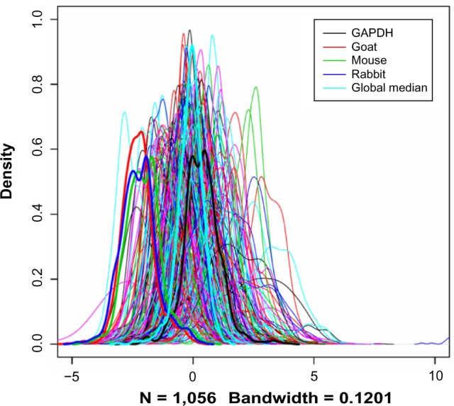
Distributions of the raw protein concentration values. Each curve corresponds to an RPPA slide (equivalent to a protein).

Notes: The curves for the three NC, the GAPDH slide, and the global median were plotted in thick lines to show their relative positions among the overall data.

Global median centering (GMC) and subtraction of a “housekeeping protein” (HK) have been discussed before,¹² but we will discuss it again for comparison. The Robust Z normalization¹⁶ (see Methods) is potentially attractive, as some statistical regressions such, as LASSO, require standardized data.¹⁷

Methods

The samples

The majority of the samples printed on the RPPA slides used in this study were solid tumor samples from The Cancer Genome Atlas (TCGA) Project (http://cancergenome.nih.gov/), and a small fraction of the samples are cancer cell lines. There are 48 control samples, 299 stomach adenocarcinoma samples, 50 Glioblastoma multiforme samples, 260 low-grade glioma samples, 164 prostate adenocarcinoma samples, 205 thyroid carcinoma samples, and 30 other samples. Most of the TCGA samples are from solid primary tumors, with a tiny fraction of metastatic samples. Per TCGAs data use policy, we have the permission to use the data before the publication of the disease-specific marker papers because the aim of the current research is development and comparison of methodologies (http://cancergenome.nih.gov/publications). All the TCGA samples are unique on the slides. The control cell line samples include two breast cell lines (MDA-MB-231 and MDA-MB-468), either control or stimulated with a growth factor, a leukemia cell line Jurkat, either control or treated with an anti-Fas agent, and a mixed lysate from multiple cell lines, with six replicates.

Lysate Preparation

Both the TCGA tumor samples and the cancer cell lines were prepared by the University of Texas MD Anderson Cancer Center RPPA Core Facility. Cellular protein concentration was determined by bicinchoninic acid reaction (Pierce, Rockford, IL). Five serial twofold dilutions were performed in lysis buffer containing 1% sodium dodecyl sulphate (SDS) (dilution buffer). The diluted lysates were spotted on nitrocellulose-coated FAST slides (Whatman, Schleicher & Schuell BioScience, Inc., Keene, NH) by a robotic GeneTAC (Genomic Solutions, Inc., Ann Arbor, MI) G3 arrayer or an Aushon Biosystems (Burlington, MA) 2470 arrayer. The antibody validation and sample preparation protocols can be found at the website of the Core Facility (http://www.mdanderson.org/education-and-research/resources-for-professionals/scientific-resources/core-facilities-and-services/functional-proteomics-rppa-core/index.html). Two hundred and three (203) proteins, including total and phosphorylated proteins, were included in this study.

Antibody Probing and Signal Detection

The DAKO (Carpentaria, CA) catalyzed signal amplification system was used for antibody blotting. Each slide was incubated with a primary antibody (Supplemental Table 1) in the appropriate dilution. The signal was captured by biotin-conjugated secondary antibody and amplified by tyramide deposition. The analyte was detected by avidin-conjugated peroxidase reactive to its substrate chromogen diaminobenzidine. Subsequently, the slides were individually scanned (Cannon Scan 9000F, Cannon U.S.A. Inc., Melville, NY) and quantitated using Array-Pro Analyzer (Media Cybernetics, Inc., Rockville, MD). This software provides automated spot identification, background correction, and individual spot intensity determination.

Estimation of Relative Protein Concentration

The R package SuperCurve was used to estimate the relative protein concentration in each dilution series. Briefly, the observed spot signal intensity data of all the dilution series on a slide are used to estimate the initial parameters of a sigmoid curve (the minimum α, the maximum β, and the slope γ). These parameters are then used to estimate the median effective concentration (EC50) for each dilution series on a given slide by solving the nonparametric model¹⁰:

$$y_{ij}=g(x_i+\mathrm{EC}{50}_j)+{\epsilon }_{ij},$$

where y_ij is the observed expression level at the ith dilution step in the jth sample, x_i is the dilution step (1 through 5 in the current experiments, and can be centered), ε_ij is the observation error, and g is an unknown function representing a nondecreasing curve. The resulting data (raw data) are in log₂ scale, and saturated and very low values are truncated (if less or higher than the maximum and minimum by two times of the SD of the residuals from model fitting).

Methods of Normalization

We compared the following eight methods for normalizing RPPA data. Some of those methods have been previously used specifically in the context of RPPA, whereas other methods are either general purpose or used in the context of gene expression data, as indicated.

Invariable protein set normalization (Inv)

In this method, the proteins are ranked in each sample, and the variance of the ranks for each marker is calculated across all the samples. The method was originally proposed for normalizing gene expression data,¹⁴ but we are proposing a variant of the method in the context of RPPA data normalization. The protein with the highest rank variance is discarded. The remaining markers are again ranked within each sample, and the protein with the highest rank variance is again discarded. The process is repeated in an iterative fashion until the number of remaining markers reaches a predetermined integer. Here we kept 100 markers. Each marker is trimmed, ie, the 25% highest values and the 25% lowest values in the entire data set are removed, and a virtual reference sample is created by averaging the remaining values of every protein across all the samples. In cases where all the values of a given protein are excluded, the top and bottom percentages need to be lowered. Each sample is normalized to the virtual reference sample by lowess smoothing using a MA-plot approach, ie, smoothing the M values (difference between the target sample and the reference sample, in log₂) against the A value (mean of the target and reference samples, in log₂), and the adjusted or normalized values are generated using the residuals of the fit.¹⁴

Loading control

In this RPPA-specific method, (i) the median expression value is subtracted from each protein (median centering); (ii) the median expression value is calculated and subtracted from the data from step (i) for each sample.^2–5,7

Tukey’s median polish

This general purpose method is essentially a nonparametric equivalent to analysis of variance. The row medians and column medians are subtracted alternately until the process converges, ie, until the proportional reduction in the sum of absolute residuals is less than a small positive number ε or until the number of iterations reaches a predetermined integer.¹⁸ The overall median is also estimated. Here we add the overall median back to the residuals as the normalized data. This should be a very robust approach if the numbers of samples and markers are reasonably large in the data. We include it only for the purpose of comparison.

Global median centering

In this RPPA-specific method, the median expression value of each sample is simply subtracted from the raw data of all the proteins for the sample.^12,19 While this may be the least “intrusive” method, ie, with fewest steps from the raw data, the sample median estimate is still biased when the number of markers is low, eg, <100.

Subtraction of HK

In this RPPA-specific method, GAPDH is used as a HK, and its value is subtracted from that of other proteins for each sample.¹²

Variable slope normalization

This RPPA-specific method regards the data for different slides as having different sigmoidal slopes from the curve estimated with common quantification methods.²⁰ The slopes are estimated and divided after the markers are median centered and before the samples are median centered.¹²

Subtraction of NC

To normalize the data, the raw protein concentration values of the NC are subtracted from the raw protein concentration values of the slides stained with antibodies from the corresponding antibody/animal source. For instance, if a slide is stained with a mouse antibody, the slide is normalized using the mouse negative control slide and the same for rabbit antibodies. NCs have been previously used for RPPA data, but in a different context in that the negative control is used as a predictor in a model.¹⁵

Robust Z normalization (Z’)

This general purpose method is the robust counterpart of the standard score.¹⁶ The normalized data for the ith protein and jth sample is calculated as:

$${X^{\prime }}_{ij}=(X_{ij}-{\text{MED}}_i)/{\text{MAD}}_i,$$

where X_ij is the raw data for the ith protein in the jth sample (j = 1, 2, …, s), and MED_i and MAD_i are the median and median absolute deviation, respectively, of the ith protein. The s can be the total number of samples on a slide or the number of samples in a sample subset.

An in Silico Experiment to Test Loading Correction

This experiment was designed to test the performances of the normalization methods regarding the fold changes between groups of samples and the distribution of sample medians. Since there are five twofold dilution steps for each sample (steps 1–5, with the lysate diluted to 100%, 50%, 25%, 12.5% and 6.25%, respectively, of the original concentration), the protein concentration from a dilution series with steps 1–4 would double that from a dilution series with steps 2–5 when estimated by Super-Curve. Therefore, we have created a pseudo-slide from each original slide by first randomly selecting half of the samples and taking the steps 1–4 and steps 2–5 of each original five-step dilution series, ie, generating a pair of pseudo-samples from each original sample [we call them high-concentration (H) and low-concentration (L) samples, respectively]. To avoid potential bias due to the proportion of the L samples, three scenarios were considered: the ratio of the number of H samples to the number of L samples was 1:1, 10:1, or 1:10. Then the fold changes were evaluated using only the paired H and L samples. We would expect that these differences will be rendered to near zero after an effective loading correction, and the median values of all the samples will be similar.

Immunohistochemistry/Florescence in Situ Hybridization Data

In breast cancer, the immunohistochemistry (IHC)/florescence in situ hybridization (FISH) measurements of three key proteins in breast cancer estrogen receptor (ER), progesterone receptor (PR), and Human Epidermal Growth Factor Receptor 2 (HER2) are usually available as part of clinical information of the patients. We took advantage of this independent data to help test our data normalization methods. The original clinical data are available at TCGA’s data portal (the file “clinical_patient_brca.txt” at https://tcga-data.nci.nih.gov/tcgafiles/ftp_auth/distro_ftpusers/anonymous/tumor/brca/bcr/biotab/clin/, as of July 2013). The positive and negative calls for ER and PR were taken directly from the file. For HER2, a sample was “positive,” “equivocal,” and “negative” if the IHC level was 3+, 2+, and 1+, respectively. For the equivocal ones, and FISH score was used to help with the decision (positive if FISH score was >2.2 and negative if FISH score was <1.8). Only the samples with clear positive and negative calls were used. We compared the mean protein expression (total protein), measured with RPPA, between the positive and the negative groups by t-statistic.

Evaluation Criteria

MA-plots were used to judge the performance of variance correction. The disperses of distributions of the sample medians and the distribution of the differences between the paired high- and low-concentration samples in the simulated data were used to evaluate the performance of loading correction. Lin’s concordance correlation coefficient (CCC)²¹ was also used to judge how the normalization methods affect the closeness between replicate samples and closely related proteins. A high CCC requires that the two variables under comparison not only have high a Pearson correlation but also have a regression line close to the line of intercept 0 and slope 1.

Results and Discussion

Distribution of the between-protein and between-sample correlations

We calculated all the pairwise Spearman correlation between the proteins and the samples and plotted them in Figure 2 (the curve from the raw data is covered by the Z’ one, as theoretically the ranks of the protein data within each sample does not change merely by that procedure). The curves in Figure 2A are the separately sorted Spearman ρ values. For the raw data, the protein–protein correlation are mostly positive and more than a half are greater than 0.5, which is an exaggeration of reality, where we expect the positive and negative correlation coefficients are largely equal. The NC and HK methods resulted in the very similar ρ values as the raw data did. The other methods, Inv, LC, median polish (MP), GMC, and VS, all reduced the protein–protein correlations to a realistic level, ie, about half positive and half negative.

Figure 2.

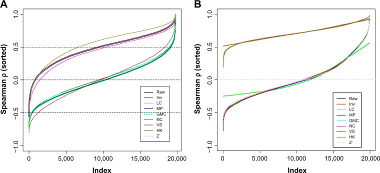
Distributions of all the pairwise correlation coefficients (Spearman ρ) between proteins (A) and between samples (B). The ρ values are sorted separately for each method in both A and B. Only 20,000 ρ values were randomly selected out of 557,040 ones (pairwise for 1056 samples) to plot in B to show the shapes of the curves.

Note: Raw: data from SuperCurve with no normalization; LC: loading control; Inv: invariant marker set normalization; MP: median polish; GMC: global median centering; NC: subtraction of negative control; VS: variable slope normalization; HK: subtraction of housekeeping protein; Z′: robust z-score. This applies to Figure 2–6.

For the pairwise sample-to-sample correlation (Fig. 2B), the ρ values from all the methods were sorted by the order of the ρ values derived from the raw data (a black line covered by other lines neat the top of the plot). All the methods other than VS, MP, and Z’ gave similar or identical results, as subtraction of a constant does not affect the ranks of the proteins in each sample (ie, LC, GMC, NC, and HK). As we will discuss later, the high sample-to-sample correlation is not as much a concern as the protein-to-protein.

Loading Correction

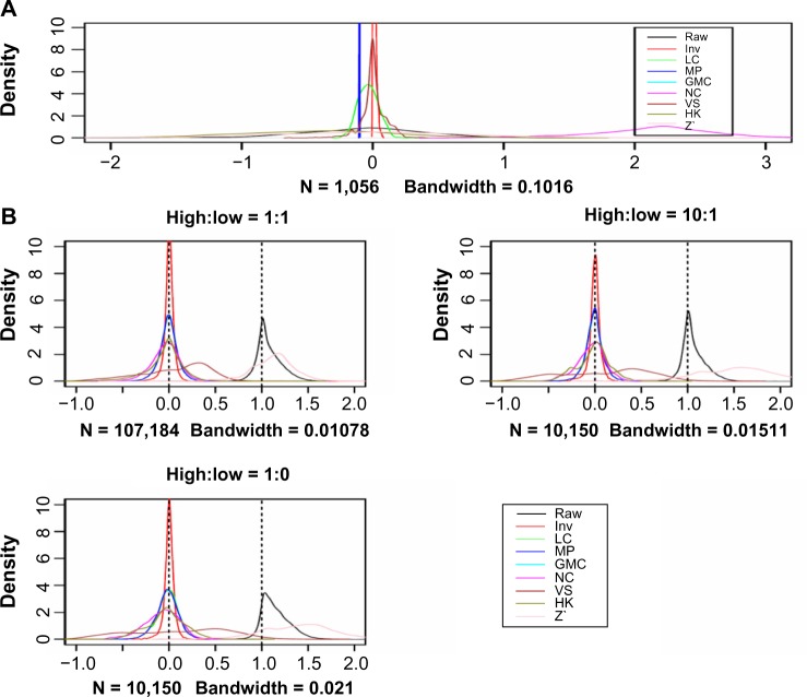
Figure 3A shows the distributions of the sample medians for the actual raw data and the normalized data using different methods. All the sample medians are centered at or near 0 except the NC one. The curves from the raw data and the HK- and Z’-normalized data are very widely dispersed. We would like to see narrower dispersions, which are an indication of more effective loading correction. In this sense, MP, VS, Inv, and LC are much better performers than HK, Z’, and NC. The GMC method inherently generates 0 medians for all samples and the curve is not shown in the figure to reduce the crowdedness of the figure.

Figure 3.

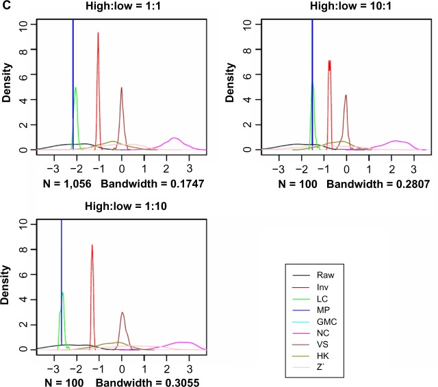
(A) Distributions of the median protein values of the 1056 samples after various normalization procedures on the actual data set; (B) distributions of the protein-level differences between the high- and low-concentration sample pairs for all the proteins (the difference data for 528, 50 and 50 pairs of samples were plotted, respectively, for the high:low = 1:1, 10:1 and 1:10 scenarios; (C) sample medians of normalized data using 1056, 100 and 100 samples, respectively.

Notes: Note that the GMC method generates 0 medians for all the samples and is not shown in the figure.

We performed an in silico experiment to test the performance of the methods. As described in the Methods section, the fold difference (twofold) was simulated at the spot signal intensity level. The densities of the differences between all the high- and low-concentration sample pairs for all the proteins were plotted in Figure 3B. We can see that the differences are essentially kept in the raw data (1 on the x-axis corresponds to twofold), although there is an overestimation in the fold change, as shown by the heavy tail on the right-hand side. All the normalization methods resulted in differences that are centered or near 0 except for the Z’ and VS methods. Of the former methods, the Inv method has the narrowest distribution next to MP. Figure 3C shows the distributions of the median protein levels of the samples. Again, the Inv and MP generated very narrow spikes, as well as LC. In both cases, MP generated very narrow peak by definition. Depending on the converging iteration the procedure ends at, the sample medians can be all 0 or a group of very similar small numbers.

Variance Stabilization

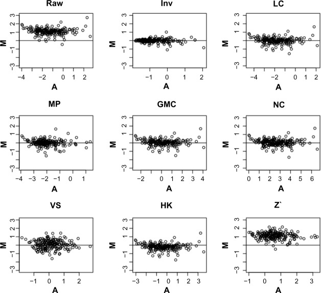
The MA-plot between pairs of control samples (duplicates from the same cell line) helps examine the variance nonlinearity problem. The first MA-plot in Figure 4 (from raw data) shows a curvature in the data cloud, and the latter does not center at 0. The Inv method had the best performance, as the data cloud is narrower and more concentrated toward the 0 line. MP and VS distorted the shape of the data cloud, and the other methods did not change the shapes of the data clouds substantially from the raw data counterpart. Table 1 shows that the variances of M values are the least for the Inv method (some methods have the same variances due to simply shifting of the data between them).

Figure 4.

MA-plots for a typical pair of control samples from the raw data and the data normalized with various methods. A = (X1 + X2)/2 and M = X1 − X2, where X1 and X2 denote the protein concentration values of the two samples in log₂. The control samples are cell lines printed on every slide mainly for quality control, and each unique cell line has at least two replicates per slide. Plotting any other pairs of control samples also gave similar patterns that support our conclusion that the Inv method performs best.

Table 1.

The variances of the differences of the normalized data for two replicate samples per cell line control on the RPPA slides (see text).

CONTROL NAMES	RAW	INV	LC	MP	GMC	NC	VS	HK	Z’
Mixed lysate	0.139	0.046	0.139	0.139	0.139	0.152	0.276	0.139	0.164
468 Control	0.137	0.039	0.137	0.137	0.137	0.147	0.335	0.137	0.199
468 EGF	0.158	0.04	0.158	0.158	0.158	0.163	0.432	0.158	0.251
231 Control	0.117	0.033	0.117	0.117	0.117	0.119	0.295	0.117	0.172
231 IGF	0.113	0.033	0.113	0.113	0.113	0.115	0.297	0.113	0.168
Jurkat control	0.114	0.029	0.114	0.114	0.114	0.114	0.27	0.114	0.159
Jurkat fas	0.12	0.036	0.12	0.12	0.12	0.12	0.292	0.12	0.166

Note: The Inv method corresponds to the least variances.

Association of the RPPA Data with IHC/FISH Data

Figure 5 shows the t-statistics from comparing the positive and negative groups for ER, PR and HER2 as measured by IHC/FISH. The t-statistics are low overall for PR. Five normalization methods, Inv, LC, MP, GMC, and NC, produced similar results for all three hormones. With the same degrees of freedom for each hormone, we simply use the t-statistic instead of the P-value for this purpose. Since this comparison is cross-platform, we put high emphasis on this test.

Figure 5.

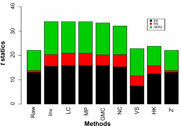
The t-statistics from comparing the mean protein values between the positive and negative groups for ER, PR, and HER2.

Note: The positive and negative calls were determined from IHC/FISH assays.

Concordance Between Replicate Samples and Closely Related Proteins

The concordance between a pair of phosphorylated proteins is very different for different proteins (Fig. 6A). Of the six pairs we have found in the data, the pAkt pair and pS6 pair have high CCC values regardless of normalization methods, and the other pairs vary dramatically. This could be due to the fact that different phosphorylation sites of the same protein can be very different events. For the concordance between replicate samples (Fig. 6B), the methods with high CCC values are essentially those that have high sample-to-sample correlations as shown in Figure 2B.

Figure 6.

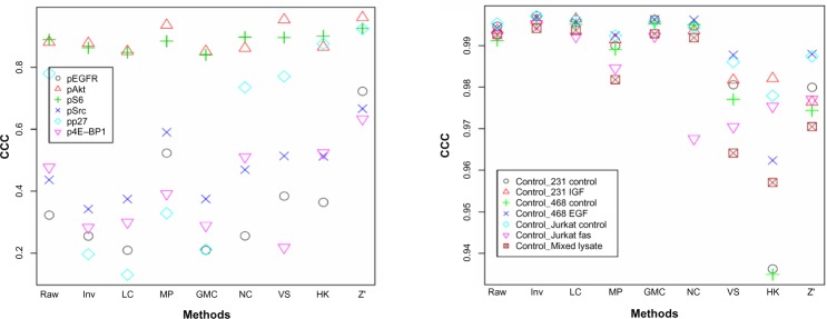
CCC between a pair of related proteins, ie, the same protein phosphorylated at different sites (A) and duplicate samples (B), after different normalization procedures.

Notes: The mixed lysate control sample have six replicates on each slide but only two replicates were used to be fair to the other six controls.

Conclusion

We have compared the performance of nine different normalization methods (including no normalization) for SuperCurve-based RPPA data. This is the first time the invariant marker set–based method has been applied on RPPA data and has performed well with respect to loading effect correction, variance stabilization, and association with IHC/FISH data. With regards to loading effect correction, the NC had wide spreads in the distributions of the sample medians and simulated high/low-concentration pair differences. The VS method, although performs well in correcting loading bias using simulated differential loadings at another level–the simulation was based on the SuperCurve output, not on the very basic level of spot signal intensity¹¹–did not perform as well in the current simulation. The rest of the methods also have strengths in one aspect and weakness in another aspect in these tests.

We consider our simulation of generating pairs of pseudo-samples a novel approach. The spatial correction step usually occurring in SuperCurve¹⁰ was not performed here because the high-concentration and low-concentration sample pair are inherently together, and they are located at randomly determined locations on the slides. An alternative is to run SuperCurve separately on the high-concentration and low-concentration samples, but the results may be not comparable.

Discussion

The fact that the fold change in the raw data is greater than 1 (log₂ scale) needs further investigation. A hypothesis is that for a five-step dilution series, the signal detection for the most diluted, eg, the fourth and fifth, spots are less sensitive than for the first few stops. If this is the case, the calculated fold changes should be lower for strong-signal pairs than for weak-signal pairs (indeed, the median difference is 1.146 for the bottom 25% weak-signal pairs and 1.003 for the top 25% strong-signal pairs).

When some proteins are high in all samples and others are low in all samples, it creates an effect similar to the sample loading effect that causes falsely high correlations between proteins. The high correlation coefficients between samples are more tolerable than between proteins in that proteins are inherently different in expression/phosphorylation levels due to biology and/or antibody affinity, although the latter cause is less desirable than the former (they are confounded and hard or impossible to separate).

There is a potential risk of over-normalization in some of these methods. For example, the MP method very effectively adjusted the loading effect and showed good correlation with the IHC/FISH data, it condensed the data spots in the MP-plot. Also, new patterns have formed in the MA-plots corresponding to VS and Z’ (Fig. 4).

To our knowledge, LC is the most commonly used method in the field, and to our comfort, it did fairly well in the three performance tests discussed earlier, but Inv performed even better: it did as well as LC in the IHC/FISH test, and better in the loading correction and variance stabilization test. In the future, we will test the algorithm on more data sets and fine-tune the parameters.

Supplementary Material

Supplementary Table 1. This file lists the antibodies used in the experiment.

REFERENCES

- 1.Paweletz CP, Charboneau L, Bichsel VE, et al. Reverse phase protein microarrays which capture disease progression show activation of prosurvival pathways at the cancer invasion front. Oncogene. 2001;20(16):1981–89. doi: 10.1038/sj.onc.1204265. [DOI] [PubMed] [Google Scholar]
- 2.Tibes R, Qiu Y, Lu Y, et al. Reverse phase protein array: validation of a novel proteomic technology and utility for analysis of primary leukemia specimens and hematopoietic stem cells. Mol Cancer Ther. 2006;5:2512–21. doi: 10.1158/1535-7163.MCT-06-0334. [DOI] [PubMed] [Google Scholar]
- 3.Liu S, Umezu-Goto M, Murph M, et al. Expression of autotaxin and lysophosphatidic acid receptors increases mammary tumorigenesis, invasion, and metastases. Cancer Cell. 2009;15:539–50. doi: 10.1016/j.ccr.2009.03.027. [DOI] [PMC free article] [PubMed] [Google Scholar]
- 4.Tsavachidou-Fenner D, Tannir N, Tamboli P, et al. Gene and protein expression markers of response to combined antiangiogenic and epidermal growth factor targeted therapy in renal cell carcinoma. Ann Oncol. 2010;21(8):1599–606. doi: 10.1093/annonc/mdp600. [DOI] [PMC free article] [PubMed] [Google Scholar]
- 5.Hennessy BT, Lu Y, Gonzalez-Angulo AM, et al. A technical assessment of the utility of reverse phase protein arrays for the study of the functional proteome in non-microdissected human breast cancers. Clin Proteomics. 2010;6:129–51. doi: 10.1007/s12014-010-9055-y. [DOI] [PMC free article] [PubMed] [Google Scholar]
- 6.The Cancer Genome Atlas Network. Comprehensive molecular portraits of human breast tumors. Nature. 2012;490:61–70. doi: 10.1038/nature11412. [DOI] [PMC free article] [PubMed] [Google Scholar]
- 7.Gonzalez-Angulo AM, Hennessy BT, Meric-Bernstam F, et al. Functional proteomics can define prognosis and predict pathologic complete response in patients with breast cancer. Clin Proteomics. 2011;8(1):11. doi: 10.1186/1559-0275-8-11. [DOI] [PMC free article] [PubMed] [Google Scholar]
- 8.Li J, Lu Y, Akbani R, et al. TCPA: a resource for cancer functional proteomics data. Nat Methods. 2013;10(11):1046–7. doi: 10.1038/nmeth.2650. [DOI] [PMC free article] [PubMed] [Google Scholar]
- 9.Dudoit S, Yang YH, Callow MJ, Speed TP. Statistical methods for identifying differentially expressed genes in replicated cDNA microarray experiments. Stat Sin. 2002;12(1):111–39. [Google Scholar]
- 10.Hu J, He X, Baggerly KA, Coombes KR, Hennessy BT, Mills GB. Non-parametric quantification of protein lysate arrays. Bioinformatics. 2007;23(15):1986–94. doi: 10.1093/bioinformatics/btm283. [DOI] [PubMed] [Google Scholar]
- 11.Neeley ES, Kornbalu SM, Baggery KA. Surface adjustment of reverse phase protein arrays using positive control spots. Cancer Inform. 2011;11:77–86. doi: 10.4137/CIN.S9055. [DOI] [PMC free article] [PubMed] [Google Scholar]
- 12.Neeley ES, Kornblau SM, Coombes KR, Baggerly KA. Variable slope normalization of reverse phase protein arrays. Bioinformatics. 2009;25(11):1384–9. doi: 10.1093/bioinformatics/btp174. [DOI] [PMC free article] [PubMed] [Google Scholar]
- 13.Li C, Wong WH. Model-based analysis of oligonucleotide arrays: expression index computation and outlier detection. Proc Natl Acad Sci USA. 2001;98:31–6. doi: 10.1073/pnas.011404098. [DOI] [PMC free article] [PubMed] [Google Scholar]
- 14.Pelz CR, Kuesz-Martin M, Bagby G, Sears RC. Global rank-invariant set normalization (GRSN) to reduce systematic distortions in microarray data. BMC Bioinformatics. 2008;9:520. doi: 10.1186/1471-2105-9-520. [DOI] [PMC free article] [PubMed] [Google Scholar]
- 15.Troncale S, Barbet A, Coulibaly L, et al. NormaCurve: a Supercurve-based method that simultaneously quantifies and normalizes reverse phase protein array data. PLoS One. 2012;7(6):e38686. doi: 10.1371/journal.pone.0038686. [DOI] [PMC free article] [PubMed] [Google Scholar]
- 16.Birmingham A, Selfors LM, Forster T, et al. Statistical methods for analysis of high-throughput RNA interference screens. Nature Methods. 2009;6:569–75. doi: 10.1038/nmeth.1351. [DOI] [PMC free article] [PubMed] [Google Scholar]
- 17.Efron B, Hastie T, Johnstone I, Tibshirani R. “Least Angle Regression” (with discussion) Ann Stat. 2004;32(2):407–99. [Google Scholar]
- 18.Tukey JW. Exploratory Data Analysis. Reading, MA: Addison-Wesley; 1977. [Google Scholar]
- 19.Byers LA, Wang J, Nilsson MB, et al. Proteomic profiling identifies dysregulated pathways in small cell lung cancer and novel therapeutic targets including PARP1. Cancer Discovery. 2012;2:798–811. doi: 10.1158/2159-8290.CD-12-0112. [DOI] [PMC free article] [PubMed] [Google Scholar]
- 20.Tabus I, Hategan A, Mircean C, et al. Nonlinear modeling of protein expressions in protein arrays. IEEE Trans Signal Process. 2006;54:2394–407. [Google Scholar]
- 21.Lin L. A concordance correlation coefficient to evaluate reproducibility. Biometrics. 1989;45:255–68. [PubMed] [Google Scholar]
Associated Data
This section collects any data citations, data availability statements, or supplementary materials included in this article.
Supplementary Materials