

Abstract
Lysozyme is a well-studied enzyme that hydrolyzes the β-(1,4)-glycosidic linkage of N-acetyl-β-glucosamine (NAG)n oligomers. The active site of hen egg-white lysozyme (HEWL) is believed to consist of six subsites, A-F that can accommodate six sugar residues. We present studies exploring the use of polarizable force fields in conjunction with all-atom molecular dynamics simulations to analyze binding structures of complexes of lysozyme and NAG trisaccharide, (NAG)3. Molecular dynamics trajectories are applied to analyze structures and conformation of the complex as well as protein-ligand interactions, including the hydrogen-bonding network in the binding pocket. Two binding modes (ABC and BCD) of (NAG)3 are investigated independently based on a fixed-charge model and a polarizable model. We also apply MM-GBSA methods based on molecular dynamics using both non-polarizable and polarizable force fields in order to compute binding free energies. We also study the correlation between RMSD and binding free energies of the wildtype and W62Y mutant; we find that for this prototypical system, approaches using the MD trajectories coupled with implicit solvent models are equivalent for polarizable and fixed-charge models.
I. INTRODUCTION
Hen Egg White Lysozyme (HEWL) hydrolyzes β-(1,4)-glycosidic bonds of N- acetyl-D-glucosamine (NAG) homo-oligomer and alternating polymers of NAG and N- acetyl-muramic acid (NAM) in peptidoglycan cell walls of Gram-positive bacteria. The substrate binds in a cleft that can accommodate six saccharide units (A-F) (See Figure 1). The widely accepted mechanisms1–3 propose the cleavage of glycosidic linkages between the D and E sites during the hydrolysis process. To study the catalytic mechanism, a series of crystal structures were determined for HEWL with various oligosaccharides4–8. As a hydrolysis product and an important substrate analogue, NAG trisaccharide, (NAG)3, was found to bind in the A, B and C sites using X-ray crystallography5,9, where (NAG)3 interacts with the protein via a stacking interaction to Trp62 and hydrogen bonds to Trp62, Trp63, Ala107, Asp1015,8. On the other hand, crystallographic studies on HEWL mutant complex structures found different binding modes of (NAG)3; the ligand is bound in the ABC site in N59D mutant as in the wildtype8 but shifts to the BCD site in both W62Y and W62F mutants5. The enhancement of BCD occupancy was considered important in explaining the higher bacteriolytic activity of W62Y and W62F mutants relative to the wildtype HEWL and N59D mutant8. Meanwhile, human lysozyme, which hydrolyzes NAG homo-polymer more effectively than HEWL, binds (NAG)3 in both ABC and BCD modes10,11, implying a binding mode effect on lysozyme catalytic activity. However, a recent X-ray powder diffraction study12 found that (NAG)3 occupied the ABC and BCD sites in the ratio of 35:65, suggesting a favorable BCD binding in the polycrystalline slurry of HEWL-(NAG)3 complex. To probe the relation between binding mode and hydrolytic activity, it is essential to determine the complex structure in solution phase, the natural environment of the hydrolysis process. To our knowledge, there is no NMR solution structure for the complex.
Figure 1.
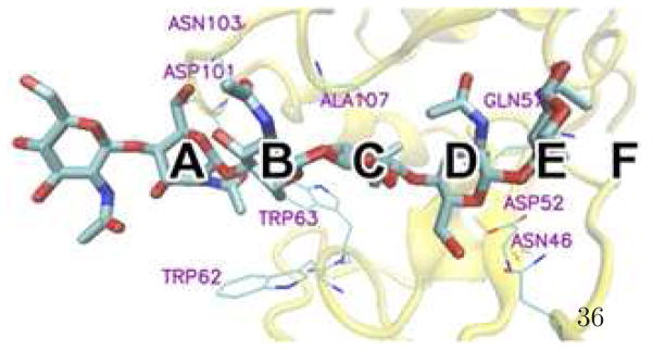
The six binding subsites of HEWL labeled A, B, C, D, E, and F.
With the development of carbohydrate force fields13,14, molecular dynamics (MD) simulations have been applied to study structural, dynamics and energetic properties of protein-sugar complex in aqueous solution15–17, but computational modeling studies are scarce for this system. Kamiya et al.17 performed a multi-canonical molecular dynamics simulation on the HEWL-(NAG)3 complex with explicit water molecules and detected a free energy barrier between the native complex structure and other structures, but the authors did not discuss the possibility of binding to the BCD site (BCD mode) and no quantitative binding free energy result was reported. Moreover, current molecular modeling studies on protein-carbohydrate complex system employ conventional fixed-charge force fields, which neglect dynamic electrostatic polarization effects during the binding process. Recent studies have addressed the effects of polarization on binding structure and free energetics using different polarizable electrostatic interaction formalisms18,19; these studies suggest that there are important contributions such non-additive effects contribute in defining structural and energetics aspects of weak interactions in the context of protein-ligand association. Efforts are also made to apply polarizable potential with implicit solvent to compute ligand binding free energies20,21.
Recently, we developed a polarizable force field for NAG molecule and compared with an existing fixed-charge force field (see reference22). Here, we apply the polarizable (non-additive electrostatic) model along with a polarizable protein force field23,24 to study the binding structure of HEWL-(NAG)3. Both ABC and BCD binding modes are constructed and simulated via molecular dynamics using both fixed-charge and the polarizable models. Protein-ligand interactions, including water-containing hydrogen bonding networks, are analyzed based on explicit solvent simulations. We also compute the binding free energy using the MM-GBSA method and explore how the binding affinity correlates with root mean squared deviation (RMSD) from existing crystal structures.
In the following, we briefly discuss the computational methodologies applied for this study. First, we describe the polarizable model based on the charge equilibration formalism, to treat partial charges as dynamical variables during the course of the simulation. The charges respond to changes in local electrostatic potential based on atomic properties of electronegativity and hardness. The approach we use to treat electrostatic polarization is one of several that are being pursued and reported in the current literature25–31. Following discussion of the force fields used for molecular dynamics simulations, we analyze the binding structure of HEWL-(NAG)3 complex and discuss our approach to implicit solvent based methods for estimating binding free energies for protein-ligand systems. We employ the MM-GBSA approach using the Generalized Born model with simple switching function to solve for the electrostatic potential in the presence of system partial charges.
II. METHODS
A. Force Fields and the Charge Equilibration Model
We perform free molecular dynamics simulations using both a fixed-charge force field and the polarizable force field for the complex in solution. To model the solvent, in this case water, we adopt the CHARMM TIP3P water model32 for the fixed-charge solution simulations and TIP4P-FQ-like (Transferable Intermolecular Potential Four Point-Fluctuating Charge) water for the CHEQ model. The TIP4P-FQ-like model used here, slightly different from the original TIP4P-FQ model31, has Lennard-Jones(LJ) sites on water hydrogens which are only in effect for water-solute interactions; this is for consistency with the CHARMM protein and small molecule CHEQ force field23. We employed the PHLB parameter set for the pyranose ring and the CHARMM22 protein force field32 for acetamido side group parameters. The protein polarizable force field based on the charge equilibration scheme23,27,28,31,33–40 (CHEQ model) was developed by Patel and Brooks23,24. The polarizable force field for the ligand based on the CHEQ model (shown in Supplementary Information Tabel 1–3), (NAG)3, was developed and the hydration free energy and other solution properties were analyzed in our previous work22.
The charge equilibration (CHEQ), or electronegativity equalization, method incorporates polarization effects within a classical molecular force field as described in the literature 23,27,28,31,33–40. Here we briefly describe the main points.
The electrostatic energy in terms of the atomic partial charges Qi as for a system of M molecules containing N atoms per molecules is then expressed as
| (1) |
The electronegativity and hardness parameters and , respectively, represent derivatives of the electrostatic energy with respect to charge while the off-diagonal interaction elements Jij(rij) describe screened Coulomb interactions between atoms i and j. In the original formulations of the method pertaining to molecular systems28,31, these were taken to be the molecular Coulomb integral over atomic Slater or Gaussian orbitals located on the respective nuclei28,31. In the current work, we apply an empirical combining rule to approximate the Coulomb overlap integral. This function depends on the individual atomic hardness parameters and interparticle distance as
| (2) |
The pair-wise energy term given by equation 1 is accumulated between atom pairs involved in bonds, angles, and dihedral (torsional) interactions within a molecule. For electrostatic interactions between intramolecular sites separated by more than four bonds, a standard Coulomb interaction applies; this is the standard protocol in most non-polarizable force fields. Intermolecular electrostatic interactions are also treated using a Coulomb form.
In order to obtain physically reasonable charge distributions, the CHEQ system of equations must be augmented by one or more additional constraints designed to conserve overall charge. For a single molecular charge constraint in which the sum of the atomic partial charges is constrained to be equal to some total charge Qnet, we require the constraint equation28,41
| (3) |
which may be added to the CHEQ energy expression in equation 1 to yield the constrained energy expression
| (4) |
The charge conservation constraint is enforced via the Lagrange multiplier λ that, when satisfied, does not contribute to the final minimized energy. The resulting energy expression is then valid for both neutral and charged systems depending on the value of Qnet. For larger molecular systems, multiple charge conservation units can be applied with separate Lagrange multipliers accounting for the individual charge constraints; for k charge normalization units, each with a net charge of Qnet,k we write:
| (5) |
During molecular dynamics simulations we propagate all charge degrees of freedom using an extended Lagrangian constrained to preserve molecular charge neutrality. The charge degrees of freedom are propagated via an extended Lagrangian formulation that imposes a molecular charge neutrality constraint, thus strictly enforcing electronegativity equalization at each dynamics step. The system Lagrangian is
| (6) |
where the first two terms represent the nuclear and charge kinetic energies, respectively, while the third term is the total potential energy including charge conservation constraints. The fictitious charge dynamics, analogous to the fictitious wave function dynamics in Car-Parrinello (CP) type methods,42 are determined with a fictitious charge “mass” (adiabaticity parameter in CP dynamics)23,31. The units for this mass are . The charges are propagated based on forces arising from the difference between the average electronegativity of the molecule and the instantaneous electronegativity at an atomic site. Accounting for charge dynamics using sufficiently small masses for the charge degrees of freedom incurs a cost of 2–4 relative to fixed-charge force fields; this arises solely from the need to use smaller timesteps.
The molecular polarizability can then be calculated as
| (7) |
where η′ is the atomic hardness matrix augmented with the appropriate rows and columns to treat the charge conservation constraints43. Rγ and Rβ are the γ and β Cartesian coordinates of the atomic position vectors (which are also augmented to appropriately match the dimensions of the atomic hardness matrix).
The nonbonded interactions are treated using a Lennard-Jones potential summed over all non-bonded atom pairs:
| (8) |
The parameters ε and Rmin correspond to the energy well depth and position of minimum potential, respectively. Bonded interactions to describe classically bond stretching, bond angle bending, torsional motions, and out-of-plane dynamics are treated using the standard CHARMM functional form44.
B. Simulation Details
Two binding modes (ABC and BCD) of HEWL-(NAG)3 complex are simulated independently in this work. The binding modes are considered as the general conformations obtained with the oligosaccharide ligand present in ABC or BCD binding pockets of the protein. ABC conformation is obtained from the X-ray crystal structure (PDB:1lzb). To construct the ligand in BCD site, the carbohydrate residue at the A site is removed from the HEWL-(NAG)4 X-ray structure bound in ABCD site (PDB:1lzc). Each of the two starting structures is solvated in an octahedral water box. Bulk solution simulations were performed within the isothermal-isobaric ensemble (NPT) at 298K and 1 bar. A constant temperature of 298K was maintained with a Hoover thermostat45,46 and constant pressure was maintained via a Langevin piston method45. Non-bonded interactions were switched to zero via a switching function from 10 to 12 A. Conditionally convergent long-range electrostatic interactions were treated using the Smooth Particle Mesh Ewald47 method with 24 grid points in each dimension and screening parameter of κ=0.32. We performed ten-nanosecond molecular dynamics simulations using a Verlet leapfrog integrator with timestep of 0.001 picoseconds (1fs) and the CHARMM22 force field. Using a polarizable force field, we simulated the solvated X-ray structure (ligand at the ABC sites) for 12 ns and the one with (NAG)3 bound to the BCD sites for 14 ns with timestep of 0.0005 ps (0.5 fs), the first 500 ps of which is considered as equilibration period. Charge degrees of freedom were maintained at 1 K using a Nose-Hoover bath; all charges were assigned to the same bath and no local “hotspots” in charge were observed. Protein, water and ligand charge degrees of freedom were assigned masses of 0.000095, 0.000069 and 0.0001 kcal mol−1 ·ps2·e−2, respectively. Charge normalization was maintained by groups for the protein and ligand and over individual molecules for the water. The charge normalization groups for the NAG residues are discussed in reference22.
C. MM-GBSA Calculations
To complement the analysis of protein-ligand interactions sampled from all-atom molecular dynamics simulations using both the polarizable and non-polarizable force fields, we consider the application of implicit solvent methods for binding free energy calculations based on sampling using MD. The binding free energy based on MM-GBSA method is:
| (9) |
ΔEMM is the difference of the gas-phase potential energy of the protein-ligand complex and individual protein and ligand in gas-phase. EMM of complex, protein and ligand are computed independently using snapshots from the molecular dynamics trajectory; we use a non-bond inter-action energy cutoff value of 9999 Å for computing electrostatic and Lennard-Jones interactions. Thus, no long-range, Ewald-type electrostatic interactions are considered (consistent with the interpretation of the molecule being in gas-phase).
The solvation free energy difference ΔGsolv contains the electrostatic contribution based on the generalized-Born method48,49 and the nonpolar contribution estimated by the molecular solvent-accessible surface area (SASA)47. The internal solute dielectric is set to be 1.0 and the solvent dielectric constant to be 80.0. For the molecular surface boundary, a half of smoothing length is 0.2 Å and the look-up table grid spacing is 1.5 Å. Atomic radii of amino acids are adopted from previous studies50, and the NAG radii are obtained from the work of Green et al.50,51. The charges used for the GBSW calculations are as follows: for the polarizable force field based simulations, the charge equilibration charges are applied for structures obtained from simulations using the polarizable force field; to reiterate, since the polarizable force field adopted for this work treats polarization via charge transfer within the molecular solute, the partial atomic charges are dynamical entities and vary during the course of the simulations. Thus, each snapshot used for the post-dynamics GBSW analysis involves a different partial charge distribution in the case of the charge equilibration (polarizable) model. For the fixed-charge CHARMM22 force field based simulations, the partial charge on each atomic site is constant for all snapshots. We acknowledge that the GB parameters we implement for this study were only optimized for the fixed-charge force field, and the accuracy of solvation free energy based on CHEQ charges may need further refinement, standardization, and/or calibration with respect to experimental solvation free energies of small molecules; this, however, is beyond the scope of this work. Here we apply the same GB radii to qualitatively probe how the electrostatic solvation free energy changes as a result of structural and charge differences between the two force fields (fixed-charge and polarizable).
Finally, the entropy change (ΔS) upon binding is computed by subtracting the free protein entropy (SP) and the free ligand entropy (SL) from the protein-ligand complex (SPL). For each species, the entropy is decoupled into vibrational, translational and rotational contributions. The vibrational entropy was estimated from independent simulations for protein, ligand and complex with explicit solvent based on the quasiharmonic approximation52. The solute entropy can also be computed from a combination of classical statistical formulas and normal-mode analysis53. The normal-mode method applies a simple harmonic model to a set of minimized structures of bound and unbound states to obtain the average entropy change without contributions from solute motion between different conformational minima53–56. As an alternative to normal-mode calculations, quasiharmonic analysis52 calculate vibrational entropy based on snapshots from a simulation trajectory; however, such entropy estimates are prone to convergence problems57,58. Harris and Laughton58 studied the convergence of the vibrational entropy of duplex DNA based on quasi-harmonic analysis using the Schlitter equation59 and found that the vibrational entropy didn’t converge over 10 ns simulation. To eliminate the time dependence arising from sampling issue, the authors extrapolated for the entropy at infinite simulation time by fitting a function to the entropy versus time profile. The entropy extrapolation method is based on the approximation that the energy landscape is smooth over the simulation and that the entropy is independent of the portion of trajectory analyzed, which in practice we acknowledge, is difficult to accomplish due to limited sampling (for our simulations, we obtain S(t) differences in the order of 10% using a sampling period of time t during the first portion of the MD trajectory, compared to using the same length of time t during a later portion of the trajectory. The expression used by Harris and Laughton as well as for this study is:
| (10) |
S(t) represents the entropy obtained from simulation time t, and the converged vibrational entropy, taken as the entropy obtained from infinite sampling, S∞ is extrapolated by fitting parameters A and n. However, based on the discussion of Harris et al58, the physical meaning of the fitting constants A and n are somewhat unresolved. Translational and rotational entropies are neglected in the calculation, assuming that the ligand binding process has little effect on the two properties58. Dynamics trajectory files are analyzed using the quasi-harmonic method in the VIBRAN module of CHARMM. Translational and rotational motions are removed from the MD trajectory files (see Supplementary Information Figure 1 for the number of structures of each system). The structures are saved every 1 ps for the fixed-charge simulations and 0.5 ps for the CHEQ model. The time-dependent entropy profiles are displayed in Supplementary Information Figure 1, suggesting the difficulty in estimating converged entropy values as observed in other studies58. For the current study, acknowledging the limitation of entropy convergence to the infinite-sampling value, we take the fitted values of S∞ as estimates of the vibrational entropy changes involved in the process we are modeling. For individual protein, ligand or protein-ligand complex in gas phase, the translational and rotational entropies are computed using the equations60,61:
| (11) |
| (12) |
where mi is the mass and and are the moments of inertia of species i (i = protein, ligand or protein-ligand complex). σi is the symmetry factor of i, which is set to be one for all species in this study.
D. Generating structures with different RMSD
Protein-ligand complex structures with different RMSD relative to the crystal structure are generated to study the correlation between binding strength and structure. We take 30 and 10 uncorrelated conformations from simulations of wildtype and W62Y mutant complex in aqueous solution, respectively. Tryptophan (Trp62) at the binding site is substituted to tyrosine (Tyr) in the W62Y mutant which leads to less favorable binding for the HEWL-(NAG)3 complex because of the loss of one hydrogen bond and the reduction of stacking interaction62. Each structure is then minimized independently with RMSD relative to the crystal structure constrained from 0 to 5 Å with an interval of 0.01 Å based on the CHARMM C22 force field. The binding free energies of these structures are computed based on the GBSW and Solvent Accessible Surface Area (SASA) methods discussed above using the CHARMM C22 force field and the current CHEQ force field.
III. RESULTS AND DISCUSSION
A. Binding Position of (NAG)3
HEWL X-ray crystallography studies suggest that (NAG)3 binds at the ABC sites9,62. An X-ray powder diffraction study12 by Von Dreele, on the other hand, suggested that (NAG)3 occupies the ABC and BCD sites in the ratio of 35:65. Von Dreele attributed the absence of BCD binding in the solid state to the hydrolysis at the CD site63. Here, we investigate the ABC and BCD complexes by two independent MD simulations starting from the crystal binding structures (see Section II A for more details).
We first calculate center of mass distances between protein heavy atoms and (NAG)3 heavy atoms as a function of time (Figure 2). Starting from the native complex structure, i.e. the ABC structure, the ligand shows no significant translational shift from the ABC sites (Figure 2 top panel). The average center of mass distance obtained from simulations using the CHARMM22 force field is 14.7 Å and 14.2 Å based on the CHEQ model, in agreement with the distance of 14.0 Å in the crystal structure. Simulations starting from the BCD structure show that the distance between (NAG)3 and HEWL is also well-maintained over the trajectories using both the CHARMM22 and the CHEQ models.
Figure 2.

Evolution of distances between center of mass of protein heavy atoms and center of mass of (NAG)3 heavy atoms obtained from trajectories based on fixed charge model (upper panel) and polarizable model (lower panel). The distance for crystal structure (1LZB) is 14.02 Å (red straight line) and shifts to 11.56 Å (red dash line) when (NAG)3 bound to the ABC sites.
To investigate structural changes of the complex over the dynamics trajectory, the root-mean-square-deviation (RMSD) profiles for HEWL backbone atoms (C, N, O atoms of the peptide bonds) (Figure 3) and (NAG)3 heavy atoms (Figure 4). The CHEQ and CHARMM22 force fields predict similar time evolution of protein backbone structure based on similar protein RMSD time profiles (averaging about 1 Å after multi-nanosecond molecular dynamics simulations) for the case where the (NAG)3 is bound in the ABC site (see Figures 3 Panel a and c). The protein backbone atom RMSDs are found to be higher with the CHEQ force field than the ones with the C22 model (see Figures 3 Panel d). To probe changes in protein structure, we further analyze the RMSD profiles for backbone atoms in helix, sheet and turn structures (residues of such structures are defined in the PDB file, PDB ID: 1LZB) as shown in Supplementary Information Figure 2 for the C22 model and Supplementary Information Figure 3 for the CHEQ model. Consistent with the all-backbone RMSD profiles (Figure 3), the fixed-charge force field predicts equilibrated RMSD profiles for the three structures with slightly larger fluctuations in the turn structure (Supplementary Information Figure 2). Based on the CHEQ model, the changes in the turn region (Supplementary Information Figure 3 Panel e and f) dominate the RMSD changes of the whole protein backbone in Figures 3 Panel c and d, while the sheet structures in the binding site are found to be stable during the course of simulation, which suggests the binding structures are equilibrated for analysis. We also observe a relaxation time up to 3 ns for the BCD structure using the CHEQ force field. Such conformational relaxation is not observed in simulations with the CHARMM22 force field (Figures 3 Panel b). We stress that in analyzing the structural behavior of the protein when (NAG)3 is bound in the BCD site, one must keep in mind that the starting BCD conformation is obtained from the crystal structure with (NAG)4 ligand since no structure with (NAG)3 in the BCD binding site is available. Thus, one may observe deviations from the exact BCD structure and simulations may require longer relaxation time for protein as the CHEQ model suggests (Figure 3 Panel d).
Figure 3.

Evolution of HEWL backbone RMSD. Upper panels (a, b): RMSDs computed with data of trajectory using fixed-charge force field. Lower panels (c, d): RMSDs calculated from snapshots based on CHEQ model.
Figure 4.

Evolution of (NAG)3 heavy atom RMSD. Upper panels (a, b): RMSDs computed with data of trajectory using fixed-charge force field. Lower panels (c, d): RMSDs calculated from snapshots based on CHEQ model.
Considering the ligand RMSD profiles (for the case of ligand binding in the ABC site, Figure 4 Panel a and c), both force field based simulations exhibit larger fluctuations and larger RMSD values in contrast to the protein backbone deviations due to molecular size. Also, both force field suggest that (NAG)3 at the ABC sites is relatively flexible and undergoes more structural changes from the starting crystal structure than the one at the BCD sites.
Based on Figures 3 and Figure 4, structural changes of the ligand contribute significantly more than the changes in the protein to the overall conformational changes of the protein-ligand complex during the course of the MD trajectories. This is consistent with the larger B factor for (NAG)3 than that for the protein in X- ray crystallography studies17. We follow such changes of (NAG)3 by computing the evolution of the RMSD of each residue of the trisaccharide referenced to the X-ray position (Supplementary Information Figure 4 for ABC structure and Supplementary Information Figure 5 for BCD structure). The CHEQ simulations, in general, show stable RMSD evolution with smaller fluctuation. In ABC sites (Supplementary Information Figure 4), both force fields suggest that the residue at the A site has higher flexibility than those at the B and C sites, consistent with assigned X-ray B-factors5, and a simulation study by Kamiya and coworkers17. The same analysis for the BCD structure using the CHARMM22 force field (Supplementary Information Figure 5 left panels) shows slightly more flexibility for NAG residue at B site, while similar stability of the three sites is indicated by the CHEQ model (Supplementary Information Figure 5 right panels). According to an X-ray crystallography study of HEWL complex with (NAG)4 bound to the ABCD site5, the average temperature factors are 24.5, 20.3 and 36.3 for NAG residues at B, C, D sites, respectively, suggesting a weaker binding at the D site. However, both force fields show no significant increase of RMSD fluctuation at the D site, implying a stronger binding for D site residues of the trisaccharide based on the force fields. A more recent X-ray crystal structure of the E35Q mutant hen egg white lysozyme with (NAG)5 at the A′ABCD site5 (the first sugar residue resides in a purely solvent-like environment adjacent to the A site which is labeled as the A′ site by the authors), on the other hand, indicates similar B factor values at B, C and D subsites and is consistent with the simulation predictions shown in Supplementary Information Figure 5.
Next, we explore the local binding interactions and compare to the corresponding crystal structure, particularly focusing on the hydrogen-bonding pattern including ligand- solvent and ligand-protein contacts at the binding site. Recent work has emphasized the importance of water/solvent in binding sites. In particular, Berne and Friesner introduced the WaterMap method to identify unfavorable waters in the binding site and they found nontrivial effect on ligand binding affinity of replacing such “dry regions” by the hydrophobic groups in the ligands64,65.
B. Hydrogen bonding network
Solute-solvent interaction defines the sugar ring conformations in aqueous solution while intra-molecular hydrogen bonding defines the glycosidic linkage of NAG22. Here, we first compute the percentages of snapshots with direct (0-water) and water-mediating (1-water and 2-water) intra-molecular hydrogen bonds out of the total number of snapshots in the trajectories using the two force fields (Table I for the ABC structure and Table II for the BCD structure). In order to perform the same calculation for the crystal structure which has no explicit hydrogen atom coordinates, the hydrogen bond for our analysis is defined between any two oxygen or nitrogen atoms within 3.2 Å of one another; no angular definition is applied. Hydrogen bonds in the crystal structure (0-water structure) are all well reproduced in the simulations, in accordance with the NAG solution study based on the same hydrogen bond definition5. Important water bridge structures with each NAG residue based on the solution simulation4–7,9, including 1-water bridge of O1-O5, O5-O6, O3-O4, 2-water bridge between O1 and O6, are only observed at some subsites, because solvent molecules are hindered by the protein. The O5-O3 hydrogen bond, one of the key contacts at the glycosidic linkage in the crystal structure5 and the solution simulation22, is well reproduced.
Table I.
Percentages of snapshots with (NAG)3 intramolecular water bridge of the ABC structure. Numbers in the bracket show the hydrogen bond distance criteria need to apply for the crystal structure to define the corresponding type of contact.
| Contacts | X-ray | C22(%) | CHEQ(%) | ||||
|---|---|---|---|---|---|---|---|
| 0-wat | 1-wat | 2-wat | 0-wat | 1-wat | 2-wat | ||
| O1A-O6A | None | 0 | 8 | 1 | 0 | 0 | 24 |
| O1B-O6B | 2w(3.31) | 0 | 0 | 42 | 0 | 2 | 0 |
| O1C-O6C | 2w(5.25) | 0 | 0 | 18 | 0 | 0 | 15 |
|
| |||||||
| O1A-O5A | 1w | 100 | 5 | 5 | 100 | 2 | 12 |
| O1B-O5B | 1w(3.98) | 100 | 4 | 15 | 100 | 0 | 2 |
| O1C-O5C | 0w | ||||||
| 1w(4.04) | 100 | 32 | 21 | 100 | 13 | 8 | |
|
| |||||||
| O3A-O4A | 0w | ||||||
| 1w(3.74) | 100 | 43 | 49 | 100 | 55 | 35 | |
|
| |||||||
| O5A-O6A | 0w | 100 | 11 | 7 | 100 | 37 | 6 |
| O5B-O6B | 0w | ||||||
| 1w(3.38) | 100 | 25 | 8 | 100 | 53 | 1 | |
| O5C-O6C | 0w | ||||||
| 1w(4.04) | 100 | 24 | 17 | 100 | 10 | 12 | |
|
| |||||||
| O6A-O3B | 0w(3.41) | 1 | 20 | 21 | 0 | 23 | 32 |
| O6B-O3C | 1w(3.79) | 0 | 2 | 0 | 3 | 68 | 3 |
|
| |||||||
| O5A-O3B | 0w | 63 | 6 | 5 | 97 | 17 | 7 |
| O5B-O3C | 0w | ||||||
| 1w(3.79) | 74 | 3 | 0 | 97 | 51 | 0 | |
Table II.
Percentages of snapshots with (NAG)3 intramolecular water bridge of the BCD structure. Numbers in the bracket show the hydrogen bond distance criteria need to apply for the crystal structure to define the corresponding type of contact.
| Contacts | X-ray | C22(%) | CHEQ(%) | ||||
|---|---|---|---|---|---|---|---|
| 0-wat | 1-wat | 2-wat | 0-wat | 1-wat | 2-wat | ||
| O1B-O6B | 2w(3.27) | 0 | 0 | 42 | 0 | 0 | 22 |
| O1C-O6C | 2w(5.40) | 0 | 0 | 65 | 0 | 0 | 1 |
| O1D-O6D | 1w | ||||||
| 2w(3.37) | 0 | 0 | 6 | 0 | 0 | 0 | |
|
| |||||||
| O1B-O5B | 1w(3.95) | 100 | 3 | 17 | 0 | 0 | 9 |
| O1C-O5C | 1w(4.71) | 100 | 21 | 15 | 1 | 0 | 0 |
| O1D-O5D | 1w | 100 | 60 | 39 | 100 | 7 | 4 |
|
| |||||||
| O5B-O6B | 0w | ||||||
| 1w | 100 | 25 | 5 | 100 | 0 | 0 | |
| O5C-O6C | 0w | ||||||
| 1w(4.70) | 100 | 18 | 20 | 100 | 24 | 3 | |
| O5D-O6D | 0w | ||||||
| 1w | 100 | 9 | 2 | 100 | 0 | 0 | |
|
| |||||||
| O3B-O4B | 0w | 100 | 32 | 28 | 100 | 49 | 32 |
|
| |||||||
| O6B-O3C | 0w(4.48) | 0 | 2 | 3 | 0 | 0 | 0 |
| O6C-O3D | 1w(3.70) | 0 | 9 | 9 | 3 | 21 | 21 |
|
| |||||||
| O5B-O3C | 0w | ||||||
| 1w(4.70) | 81 | 3 | 0 | 97 | 15 | 0 | |
| O5C-O3D | 0w | ||||||
| 1w(3.70) | 81 | 1 | 4 | 96 | 6 | 3 | |
Hydrogen bonding contacts between ligand and protein residues are displayed in Tables III and IV for the ABC and BCD structures, respectively. We list contacts that are observed either in the crystal structure or in more than half of the complex snapshots taken from the simulation trajectory (C22 or CHEQ) in the form of 0-water, 1-water or 2- water bridge. For a complete picture of hydrogen bonding network based on Tables III and IV, schematic plots for the ligand-protein contacts are shown in Figures 5 and 6 for ABC and BCD structures, respectively. The red dashed lines represent a direct hydrogen bond, green, 1-water bridge, and blue, 2-water bridge interactions. A significant number of hydrogen bond pairings found in the X-ray structure are maintained in the simulations using both force fields. Some contacts are mediated by more water molecules, such as O6B -Asp101 and O6C -Asp48; direct and 1-water bridge hydrogen bonds in the crystal structure become one and/or two water involving hydrogen bond networks in most snapshots of the simulations. The enhancement of solvent effects in ligand-protein interactions may reveal more complex binding in biologically relevant aqueous solutions than in the solid-state crystal structures. The A site residue is found to have less hydrogen bond contacts, which explains the high RMSD variation (Supplementary Information Figure 4) and high B factor of that residue in the X-ray structure of the complex5,17. On the other hand, simulations indicate that the BCD mode has significant amount of hydrogen bond contacts to accommodate (NAG)3, and the solvent mediating hydrogen bonds are mostly found for the ligand residue at the D site because of solvent accessibility in the cleft-shaped binding site.
Table III.
Percentages of snapshots with protein-ligand hydrogen bond contact in the ABC binding site. Numbers in the bracket show the hydrogen bond distance criteria need to apply for the crystal structure to define the corresponding type of contact.
| Contacts | X-ray | C22(%) | CHEQ(%) | ||||
|---|---|---|---|---|---|---|---|
| 0-wat | 1-wat | 2-wat | 0-wat | 1-wat | 2-wat | ||
| NA -Asp101 | 0w | 0 | 24 | 19 | 20 | 15 | 5 |
| O6B-Asp101 | 0w | 22 | 43 | 58 | 63 | 13 | 12 |
| O6A-Asn103 | 0w | 3 | 7 | 13 | 0 | 8 | 6 |
| O6C-Trp62 | 0w | 58 | 11 | 6 | 51 | 27 | 18 |
| O7C-Asn59 | 0w | 77 | 0 | 3 | 58 | 0 | 0 |
| NC -Ala107 | 0w | 74 | 0 | 0 | 7 | 2 | 4 |
| O3C-Trp63 | 0w(3.31) | 85 | 0 | 0 | 95 | 2 | 0 |
|
| |||||||
| O1C-Asp52 | 1w | 0 | 76 | 60 | 7 | 76 | 13 |
| O1C-Gln57 | 1w | 0 | 74 | 75 | 3 | 85 | 6 |
| O1C-Val109 | 1w(3.62) | 0 | 47 | 35 | 0 | 0 | 51 |
| O6C-Asp48 | 1w | 0 | 1 | 51 | 0 | 2 | 41 |
| O6C-Asn59 | 1w | 0 | 28 | 29 | 3 | 33 | 11 |
|
| |||||||
| O6B-lle98 | 2w | 0 | 0 | 19 | 0 | 0 | 45 |
| O6B-Gly104 | 2w | 0 | 0 | 4 | 0 | 9 | 40 |
| O1C-Glu35 | 2w(3.39) | 0 | 4 | 83 | 0 | 7 | 70 |
| O1C-Leu56 | 2w(4.96) | 0 | 0 | 51 | 0 | 0 | 0 |
| O1C-Ala110 | 2w(5.11) | 0 | 0 | 73 | 0 | 0 | 0 |
| O3C-lle98 | 2w(3.79) | 0 | 0 | 0 | 0 | 0 | 42 |
| O3C-Gly104 | 2w(3.79) | 0 | 0 | 0 | 0 | 7 | 40 |
Table IV.
Percentages of snapshots with protein-ligand hydrogen bond contact in the BCD binding site. Numbers in the bracket show the hydrogen bond distance criteria need to apply for the crystal structure to define the corresponding type of contact.
| Contacts | X-ray | C22(%) | CHEQ(%) | ||||
|---|---|---|---|---|---|---|---|
| 0-wat | 1-wat | 2-wat | 0-wat | 1-wat | 2-wat | ||
| O6B -Asp101 | 0w | ||||||
| 2w | 12 | 61 | 50 | 2 | 90 | 32 | |
| O6C -Trp62 | 0w | 46 | 14 | 8 | 49 | 28 | 18 |
| O7C -Asn59 | 0w | 89 | 0 | 0 | 85 | 0 | 0 |
| O3C -Trp63 | 0w(3.29) | 80 | 0 | 0 | 100 | 0 | 0 |
| O6D -Glu35 | 0w | 66 | 11 | 3 | 44 | 0 | 0 |
| O6D -Val109 | 0w(3.79) | 75 | 0 | 0 | 61 | 0 | 0 |
|
| |||||||
| O1C -Asp52 | 0w(4.02) | 0 | 79 | 23 | 0 | 7 | 0 |
| NC -Ala107 | 1w | 65 | 0 | 0 | 1 | 0 | 0 |
| O1D -Glu35 | 1w | 0 | 65 | 60 | 0 | 29 | 27 |
| O1D -Asp52 | 1w(3.64) | 0 | 72 | 55 | 5 | 58 | 9 |
| O1D -Gln57 | 1w | 0 | 63 | 39 | 0 | 54 | 8 |
| O5D -Glu35 | 1w | 0 | 68 | 31 | 1 | 7 | 2 |
| ND -Asn46 | 0w | ||||||
| 1w(3.74) | 2 | 73 | 35 | 0 | 40 | 1 | |
| ND -Asp52 | 0w(4.13) | ||||||
| 1w(5.17) | 0 | 71 | 34 | 0 | 72 | 0 | |
|
| |||||||
| O6B -lle98 | 2w | 0 | 1 | 49 | 0 | 0 | 28 |
| O6B Gly104 | 2w | 0 | 0 | 21 | 0 | 0 | 7 |
| O6C-Asp52 | 2w(3.70) | 0 | 0 | 72 | 0 | 0 | 4 |
Figure 5.

Hydrogen bond network of (NAG)3 at the ABC site. Red: hydrogen bond; green: 1-water bridge; blue: 2-water bridge.
Figure 6.

Hydrogen bond network of (NAG)3 at the BCD site. Red: hydrogen bond; green: 1-water bridge; blue: 2-water bridge.
C. Stacking Interaction
Previous studies5,62 demonstrated the importance of a stacking interaction between the ligand and Trp62 with regard to protein-carbohydrate binding and hydrolytic activity. We compute the center of mass distance between Trp62 and (NAG)3 heavy atoms (Figure 7) and compare to the crystal structure position (red straight lines). Kamiya et al.17 considered a hydrophobic contact forming between an amino acid and a sugar residue when the center of mass distance between the side-chain and the gluco-pyranose ring is smaller than 6.5 A. They reported that more than 97% of “the natively bound structures” (457 natively bound structures out of 993 conformations generated by McMD at 300K in that study for the ABC structure) reproduced the hydrophobic contact between the Trp62 side-chain and the sugar ring at B and C sites, respectively. Using the same interaction definition for the ABC structure, we find that only 28 structures out of 16000 obtained from a dynamics trajectory based on the polarizable model lose such hydrophobic contacts for the carbohydrate residue at the B site and only 17% of the conformations lose this hydrophobic contact at the C site, suggesting that the force field well reproduces the interactions with Trp62. According to structures generated by the fixed-charge force field, the percentages of conformations missing these interactions are 3% and 57%, respectively. When (NAG)3 binds to the BCD sites (blue in Figure 7), the structures of complexes obtained using the nonpolarizable model show longer distance between Trp62 and the ligand relative to the distance in the ABC structure suggested by both models.
Figure 7.

Evolution of distances between center of mass of Trp62 heavy atoms and center of mass of (NAG)3 heavy atoms obtained from trajectories based on fixed charge model (upper panel) and polarizable model (lower panel). The distance for crystal structure (1LZB) is 14.02 Å (red straight line) and shifts to 11.56 Å (red dash line) when (NAG)3 bound to the ABC sites.
D. MM-GBSA Binding Free Energy
Table V shows the binding free energies of ABC and BCD binding modes based on the C22 and CHEQ model (See Section II C for more details). The interaction energy, ΔEMM, is stronger when the ligand occupies the BCD site under the same model, which is consistent with the more stable ligand RMSD profile in Figure 4 and smaller distance to the hydrophobic contact Trp62 in Figure 9. On the other hand, the CHEQ force field predicts more favorable interaction energy ΔEMM, in agreement with the shorter ligand-protein distance (Figure 2) and smaller ligand RMSD changes (Figure 3).
Table V.
Binding free energy of ABC and BCD using MM-GBSA method.
| (kcal/mol) | ABC | BCD | ||
|---|---|---|---|---|
| C22 | CHEQ | C22 | CHEQ | |
| ΔEMM | −55.70 (6.82) | −93.00 (9.01) | −78.01 (5.83) | −117.09 (5.85) |
| ΔGGB | 46.78 (18.12) | 81.12 (9.83) | 70.04 (8.90) | 87.97 (5.85) |
| ΔGSA | 2.43 (1.05) | 7.09 (1.84) | 5.21 (0.86) | 8.11 (0.61) |
| ΔGbind − TΔS | −6.49 (19.39) | −4.79 (13.46) | −2.76 (10.67) | −21.01 (8.30) |
| TΔSvib | 97.54 | 58.85 | 63.45 | 92.49 |
| TΔStrans+rot | −20.07 (0.82) | −20.25 (0.47) | −20.08 (0.84) | −20.26 (0.47) |
| ΔGbind | −83.96 (19.41) | −43.39 (13.47) | −46.13 (10.70) | −93.24 (8.31) |
Figure 9.

Binding free energy ΔGbind, interaction energy ΔEMM and solvation free energy ΔGsolv for 15000 wildtype structures.
Electrostatic solvation free energies are computed based on the generalized-Born with simple switching (GBSW) model using Green’s parameters51 for ligand, which was optimized for saccharide charges in the CSFF force field66, and CHARMM atomic radii50 for protein. The same GBSW parameters are adopted without modification for CHEQ charges. We reiterate that the current study aims to explore the nature of the currently available parameterization of implicit models for use with the existing generation of the CHARMM CHEQ force field. Further work to develop fully self-consistent implicit solvent parameters for use with the CHEQ charges is ongoing. However, to provide some context within which to consider the results of the free energy calculations presented here, we computed GB electrostatic solvation energies for model compounds as a test. Comparisons are made for GB energies of 14 small molecules using the same parameters of the C22 force field (GB radii) and CHEQ charges (Supplementary Information Table 4). GBSW energy is computed for a single structure of the solute molecule. The solute molecule is solvated in a cubic box containing 216 TIP4P-FQ water molecules and the solution is equilibrated to obtain the solute structure and CHEQ charge for GBSW calculation. The CHEQ charges on polar molecules predict more favorable electrostatic solvation free energy in the current GBSW model relative to the fixed-charge model. Only two out of 14 molecules (ethylamine and butane) show less negative GB energies based on the CHEQ charges. We note that the GB calculation in this work is for qualitative comparison and parameter refinement is needed for accurate estimation of the binding free energy.
The binding free energy reproduces the sign of experiment result of −6.6 kcal/mol62. If the entropy contribution is eliminated as suggested by other studies67–69, which is difficult to calculate and converge (see Section II C and Supplementary Information Figure 1), the results agree with experiment qualitatively for the ABC structure using both models and the BCD structure with C22 force field.
The fitting constants for the vibrational entropies are shown in Supplementary Information Table 4, which suggest positive vibrational entropy change (ΔSvib upon binding, consistent with other binding free energy study based on implicit solvent simulations70,71. The translational and rotational entropy changes are negative because the bound complex loses translational and rotational degrees of freedom comparing to the free protein and ligand.
Simulations on the nanosecond scale using both polarizable and fixed-charge force fields support the X-ray powder diffraction observation of both ABC and BCD binding structures12. Moreover, (NAG)3 RMSD profile suggests a stronger binding environment at the BCD position with hydrogen bond and hydrophobic interaction contacts, because of higher flexibility of the NAG residue at the A site. The most recent X-ray crystallography study62 on HEWL/(NAG)3 complex attributed the discontinuous electron density at the D site of the |Fo|−|Fc| map to the presence of solvent. However, we think that the possibility of ligand existence cannot be excluded because of the strong electron densities at the D site. The discontinuity of D site electron density may suggest multiple occupancies of the ligand sites (i.e., the ligand is bound in the positions ABC and BCD in some ratio) of the complex and it may also be a result of limited number of data processed (15,070 independent reflections with 75.5% completeness). One may calculate the possibility of BCD binding according to the electron densities of the |Fo|−|Fc| map; however, we failed to do so because of the inaccessibility of corresponding data. Here, we attribute the absence, or possibly weak presence, of BCD binding in the X-ray crystal structure to subsequent hydrolysis: (NAG)3 that binds to the BCD site is close to the catalytic acid/base Glu35 and may diffuse to the DE site and undergo hydrolysis during the crystallization procedure. (NAG)4, with larger molecular size, is kinetically hindered in its path to the DE site; this enables ABCD occupancy in the solid state.
E. Correlation between binding free energy and RMSD
After probing the binding modes of the native complex structure, we investigate the correlation between the binding free energy and RMSD relative to the crystal structure. Such correlation is plausible because it proves the ability of the two force fields to assign better energy scores to known high-affinity conformations. Such ability enables the modeling method to predict accurate bound complex poses and potential ligands using a simple scoring function. We generated 5000 conformations for the wildtype (ABC mode) and 5000 for W62Y mutant complex structure by minimizing the atom positions and charges with RMSD restraint in CHARMM (See Section II A for details). The binding free energy and RMSD of the binding site are computed for these conformations and displayed in Figure 8. The low binding energy structures sampled for both complexes have low RMSD (<0.5) relative to the X-ray structures (PDB:1lzb and 1lze). The energy increases for conformations with very low RMSD (<0.01), implying a structural relaxation according to the force field. Experimentally, a fluorescence spectra study found that the replacement of Trp62 with Tyr led to enhanced bacteriolytic activity and a lower binding constant for chitotriose62. The binding free energy of (NAG)3 to HEWL wildtype is 1 kcal/mol lower than that of (NAG)3 binding to W62Y. Consistently, the minimum binding free energy in Figure 10 indicates a stronger binding of (NAG)3 to HEWL than to mutant lysozyme, qualitatively reproducing the relative affinity of the wildtype and W62Y to the ligand. This observation reveals that this docking and scoring and more interactions (leading to overall stronger binding contacts and higher effective kinetic barrier between binding sites) approach based on CHEQ model not only yields high-affinity binding poses but also captures the binding energy change corresponding to a mutagenesis at the binding site.
Figure 8.

RMSD and binding free energy for the wildtype (PDB:lzb) and W62Y mutant (PDB:1lze) based on the C22 model and the CHEQ model.
In order to confirm the convergence of RMSD and binding free energy correlation, we generate 10000 more structures for the wildtype complex with different RMSD as shown in Figure 9. The general correlation persists, demonstrating that the force fields favor the crystal binding structure as discussed above. To decouple the binding free energy contributions, the interaction energy ΔEMM, and the solvation free energy ΔGsolv of each conformation are also shown in Figure 9. Both C22 and CHEQ force field predict favorable interaction energies for complex structures with small RMSD but there is another interaction energy (ΔE) minimum around RMSD 0.8 using the fixed-charge model, which disappears in the binding free energy figure (Figure 9 panel a) because of the solvation energy contribution; this observation, in conjunction with the recent attention on the energetics of water in binding pockets, speaks to the importance of including solvation effects in scoring functions that attempt to discriminate between multiple random configurations (poses) of protein-ligand complexes on the basis of structure-energy relationships. The solvation free energy ΔGsolv, on the other hand, decreases with increasing RMSD, a trend that can be attributed to the electrostatic solvation free energy change ΔGGB and the nonbond solvation free energy change contribution (Solvent Accessible Surface Areas, SASA, term), ΔGSASA. ΔGGB and ΔGSASA of complex, protein and ligand, individually, are plotted as a function of the complex RMSD in Supplementary Information Figure 6 and 7 showing the same trend as that in Figure 9 panels e and f. The complex solvation free energies, ΔGGB complex and ΔGSASA complex, (Supplementary Information Figure 6 and 7 upper panels) defines the trend of the solvation free energy ( ) because stronger correlation is found for complex free energies with RMSD. For small RMSD complex structures, the conformation and the charge (in the CHEQ model) vary to a greater extent due to the stronger interaction between protein and ligand and lead to a less favorable solvation free energy compared to the larger RMSD structures. On the other hand, with a significantly greater number of structures, we observe a new binding free energy minimum near RMSD = 1 using the CHEQ force field (Figure 9 Panel b); this implies a possibly flat region in the energy landscape of HEWL-(NAG)3 binding in the solution environment. To understand the new binding free energy minimum suggested by the CHEQ model, we analyzed the distributions of binding free energy ΔGbind, interaction energy ΔEMM and solvation free energy ΔGsolv for structures in different RMSD regions (Supplementary Information Figure 8). A broad distribution of ΔGbind in 1 ≤ RMSD < 2 region overlaps with the distribution of RMSD less than 1 and forms the new minimum in Figure 9 Panel b, which may be attributed to smaller difference of the interaction energy distributions in the two regions. More importantly, the probability of favorable binding free energy is higher in the low RMSD region ensuring that the CHEQ model can predict good binding structures according to the binding free energies. Comparing to the fixed-charge force field, the CHEQ model suggests more favorable binding free energy ΔGbind, because the solvation free energies ΔGsolv using the current GBSW model are reduced by the CHEQ charges and compensate the less favorable interaction energy ΔEMM.
IV. CONCLUSIONS
We explored two binding positions (ABC and BCD) of (NAG)3 in HEWL using a fixed-charge force field (CHARMM C22) and a polarizable force field (charge equilibration, CHEQ) for protein, solvent, and the polysaccharide ligand, N- acetyl-glucosamine (NAG). The molecular dynamics simulations suggest that the ligand binds to both the ABC and the BCD sites. The crystal structure properties, including center of mass distance, RMSD profile, hydrophobic contact, hydrogen bonding network, are well maintained by the two force fields. The local interactions between HEWL and (NAG)3 involve more solvent molecules relative to the crystal structures. Qualitative trends in experimental binding free energies of wildtype and W62Y are reproduced using MM-GBSA method. The CHEQ model predicts stronger binding free energies compared to the CHARMM22 force field. However, neither model captures the absolute binding free energy of the wildtype complex (−6.6 kcal/mole) or the mutant (−5.6 kcal/mole) based on biochemical measurements62. Interestingly, the binding free energy correlates with root mean squared deviation from the crystal structure of the protein-ligand complex, suggesting that the force fields favor the complex structures close to the crystal structure. The dominant contribution defining the trend in the correlation of MM-GBSA binding free energy with protein-ligand structural RMSD relative to the crystal structure is the molecular mechanics energy, EMM, which accounts for intramolecular and local intermolecular interactions between the ligand and local protein residues. We find also that the use of the solvation free energy contribution to the free energy of binding using MM-GBSA is necessary for this system. We will report on binding free energetics in this system using fixed-charge and non-additive, polarizable force fields in a future publication.
Supplementary Material
Acknowledgments
We thank Dr. Ying H. Pan of University of Delaware for helpful discussions of crystallographic results interpretation. The authors also acknowledge generous financial support from the National Institutes of Health (COBRE:5P20RR017716-07) at the University of Delaware, Department of Chemistry and Biochemistry. The authors are also grateful for a COBRE grant providing computational resources awarded to the Chemical Engineering Department (COBRE-3P30RR031160).
References
- 1.Phillips D. Sci Amer. 1966;215:78–90. doi: 10.1038/scientificamerican1166-78. [DOI] [PubMed] [Google Scholar]
- 2.Phillips D. Proc Natl Acad Sci USA. 1967;57:484–495. [Google Scholar]
- 3.Vocadlo D, Davies G, Laine R, Withers S. Nature. 2001;412:835–838. doi: 10.1038/35090602. [DOI] [PubMed] [Google Scholar]
- 4.Imoto T, Johnson LN, North A, Phillips D, Rupley J. Vertebrate lysozyme. In: Boyer P, editor. The Enzymes. Vol. 7. Academic Press; New York: 1972. pp. 665–868. [Google Scholar]
- 5.Maenaka K, Matsushima M, Song H, Sunada F, Watanabe K, Kumagai I. J Mol Biol. 1995;247:281. doi: 10.1006/jmbi.1994.0139. [DOI] [PubMed] [Google Scholar]
- 6.Johnson L, Cheetham J, McLauphlin P, Archarya K, Barford D, Phillps D. Curr Topics Microbiol Immunol. 1988;139:81–134. doi: 10.1007/978-3-642-46641-0_4. [DOI] [PubMed] [Google Scholar]
- 7.Strynadka K, James M. J Mol Biol. 1991;220:401–424. doi: 10.1016/0022-2836(91)90021-w. [DOI] [PubMed] [Google Scholar]
- 8.Ose T, Kuroki K, Matsushima M, Maenake K, Kumagai I. J Biochem. 2009;146:651. doi: 10.1093/jb/mvp110. [DOI] [PubMed] [Google Scholar]
- 9.Cheetham JC, Artymiuk PJ, Phillips DC. J Mol Biol. 1992;224:613. doi: 10.1016/0022-2836(92)90548-x. [DOI] [PubMed] [Google Scholar]
- 10.Benyard S. PhD thesis. University of Oxford; 1973. [Google Scholar]
- 11.Matsushima M, Inaka K, Morikawa K. Acta Crystallogr sect A. 1990;46:C82. [Google Scholar]
- 12.Von Dreele RB. Acta Cryst. 2005;D61:22. doi: 10.1107/S0907444904025715. [DOI] [PubMed] [Google Scholar]
- 13.Woods RJ, Dwek RA, Edge CJ. J Phys Chem. 1995;99:3832. [Google Scholar]
- 14.Guvench O, Greene SN, Kamath G, Brady JW, Venable RM, Pastor RW, MacKerell AD., Jr J Comp Chem. 2008;29:2543. doi: 10.1002/jcc.21004. [DOI] [PMC free article] [PubMed] [Google Scholar]
- 15.Konidalaa P, Niemeyer B. Biophys Chem. 2007;128:215–230. doi: 10.1016/j.bpc.2007.04.006. [DOI] [PubMed] [Google Scholar]
- 16.Vorontsov I, Miyashita O. Biophys. 2009;97:2532–2540. doi: 10.1016/j.bpj.2009.08.011. [DOI] [PMC free article] [PubMed] [Google Scholar]
- 17.Kamiya N, Yonezawa Y, Nakamura H, Higo J. Proteins. 2007;70:41. doi: 10.1002/prot.21409. [DOI] [PubMed] [Google Scholar]
- 18.de Courcy B, Piquemal JP, Garbay C, Gresh N. J Am Chem Soc. 2010;132:3312–3320. doi: 10.1021/ja9059156. [DOI] [PubMed] [Google Scholar]
- 19.Jiao D, Golubkov PA, Darden TA, Ren P. PNAS. 2008;105:6290–6295. doi: 10.1073/pnas.0711686105. [DOI] [PMC free article] [PubMed] [Google Scholar]
- 20.Yang T, Wu JC, Wang CYY, Luo R, Gonzales MB, Dalby KN, Ren P. Proteins: Struc, Funct, Genet. 2011;79:1940–1951. doi: 10.1002/prot.23018. [DOI] [PMC free article] [PubMed] [Google Scholar]
- 21.Jiao D, Zhang J, Duke R, Li G, Schnieders MJ, Ren P. J Comput Chem. 2009;30:1701–1711. doi: 10.1002/jcc.21268. [DOI] [PMC free article] [PubMed] [Google Scholar]
- 22.Zhong Y, Bauer BA, Patel S. J Comp Chem. 2011;32:3339. doi: 10.1002/jcc.21873. [DOI] [PMC free article] [PubMed] [Google Scholar]
- 23.Patel S, Brooks CL., III J Comp Chem. 2004;25:1. doi: 10.1002/jcc.10355. [DOI] [PubMed] [Google Scholar]
- 24.Patel S, MacKerell AD, Jr, Brooks CL., III J Comp Chem. 2004;25:1504–1514. doi: 10.1002/jcc.20077. [DOI] [PubMed] [Google Scholar]
- 25.Lamoureux G, MacKerell AD, Jr, Roux B. J Chem Phys. 2003;119:5185. doi: 10.1063/5.0019987. [DOI] [PMC free article] [PubMed] [Google Scholar]
- 26.Lamoureux G, Roux B. J Chem Phys. 2003;119:3025. [Google Scholar]
- 27.Patel S, Brooks CL., III Mol Simul. 2004;32:231. [Google Scholar]
- 28.Rappe AK, Goddard WA. J Phys Chem. 1991;95:3358. [Google Scholar]
- 29.Ren P, Ponder JW. J Comp Chem. 2002;23:1497–1506. doi: 10.1002/jcc.10127. [DOI] [PubMed] [Google Scholar]
- 30.Ren P, Ponder JW. J Phys Chem B. 2003;107:5933–5947. [Google Scholar]
- 31.Rick SW, Stuart SJ, Berne BJ. J Chem Phys. 1994;101:6141. [Google Scholar]
- 32.MacKerell AD, Jr, et al. J Phys Chem B. 1998;102:3586. doi: 10.1021/jp973084f. [DOI] [PubMed] [Google Scholar]
- 33.Rick SW, Berne BJ. J Am Chem Soc. 1996;118:672. [Google Scholar]
- 34.Sanderson RT. Chemical Bonds and Bond Energy. 2. Acedemic Press; New York: 1976. [Google Scholar]
- 35.Sanderson RT. Science. 1951;114:670. doi: 10.1126/science.114.2973.670. [DOI] [PubMed] [Google Scholar]
- 36.Chelli R, Procacci P. J Chem Phys. 2002;117:9175. [Google Scholar]
- 37.Itskowitz P, Berkowitz ML. J Phys Chem A. 1997;101:5687. [Google Scholar]
- 38.Rick SW, Stuart SJ, Bader JS, Berne BJ. J Mol Liq. 1995;31:65. [Google Scholar]
- 39.Rick SW. J Chem Phys. 2001;114:2276. [Google Scholar]
- 40.Rick SW, Stuart SJ. Potentials and Algorithms for Incorporating Polarizability in Computer Simulations. In: Lipkowitz KB, Boyd DB, editors. Reviews in Computational Chemistry. Wiley; New York: 2002. p. 89. [Google Scholar]
- 41.Mortier WJ, Ghosh SK, Shankar S. J Am Chem Soc. 1986;108:4315. [Google Scholar]
- 42.Car R, Parrinello M. Phys Rev Lett. 1985;55:2471–2474. doi: 10.1103/PhysRevLett.55.2471. [DOI] [PubMed] [Google Scholar]
- 43.Davis JE, Warren GL, Patel S. J Phys Chem B. 2008;112:8298–8310. doi: 10.1021/jp8003129. [DOI] [PubMed] [Google Scholar]
- 44.Brooks BR, et al. J Comp Chem. 2009;30:1545–1614. doi: 10.1002/jcc.21287. [DOI] [PMC free article] [PubMed] [Google Scholar]
- 45.Allen MP, Tildesley DJ. Computer Simulation of Liquids. Clarendon Press; Oxford: 1987. [Google Scholar]
- 46.Martyna GJ, Klein ML, Tuckerman M. J Chem Phys. 1992;97:2635. [Google Scholar]
- 47.Hasel W, Hendrickson T, Still W. Tetrahedron Computer Methodology. 1988;1:103–116. [Google Scholar]
- 48.Im W, Feig M, Brooks CL., III Biophys J. 2003;86:3329. doi: 10.1016/S0006-3495(03)74712-2. [DOI] [PMC free article] [PubMed] [Google Scholar]
- 49.Im W, Lee M, Brooks I, CL J Comput Chem. 2003;24:1691–1702. doi: 10.1002/jcc.10321. [DOI] [PubMed] [Google Scholar]
- 50.Nina M, Roux B. J Phys Chem B. 1997;101:5239–5248. [Google Scholar]
- 51.Green DF. J Phys Chem B. 2008;112:5238. doi: 10.1021/jp709725b. [DOI] [PubMed] [Google Scholar]
- 52.Karplus M, Kushick JN. Macromolecules. 1981;14:325. [Google Scholar]
- 53.Srinivasan J, Cheatam TC, III, Cieplak P, Kollman PA, Case DA. J Am Chem Soc. 1998;120:9401. [Google Scholar]
- 54.Gilson MK, Zhou H. Annu Rev Biophys Struct. 2007;36:21. doi: 10.1146/annurev.biophys.36.040306.132550. [DOI] [PubMed] [Google Scholar]
- 55.Kuhn B, Gerber P, Schulz-Gasch T, Stahl M. J Med Chem. 2005;48:4040–4048. doi: 10.1021/jm049081q. [DOI] [PubMed] [Google Scholar]
- 56.Mossova I, Kollman PA. Prerspectives in Durg Discovery and Design. 2000;18:113–135. [Google Scholar]
- 57.Gohlke H, Case D. J Comput Chem. 2004;25:238–250. doi: 10.1002/jcc.10379. [DOI] [PubMed] [Google Scholar]
- 58.Harris S, Laughton C. J Phys Condens Matter. 2007;19:1–14. doi: 10.1088/0953-8984/19/7/076103. [DOI] [PubMed] [Google Scholar]
- 59.Schlitter J. Chem Phys Lett. 1993;215:617–621. [Google Scholar]
- 60.McQuarrie DA. Statistical Thermodynamics. University Science Books; Mill Valley, CA: 1973. [Google Scholar]
- 61.Tidor B, Karplus M. J Mol Biol. 1994;238:405. doi: 10.1006/jmbi.1994.1300. [DOI] [PubMed] [Google Scholar]
- 62.Kumagai I, Sunada F, Takeda S, Miura K. J Biol Chem. 1992;267:4608. [PubMed] [Google Scholar]
- 63.Rupley J, Gates V. Proc Natl Acad Sci USA. 1967;57:496–510. [Google Scholar]
- 64.Abel R, Young T, Farid R, Berne B, Friesner R. J Am Chem Soc. 2008;130:2817–2831. doi: 10.1021/ja0771033. [DOI] [PMC free article] [PubMed] [Google Scholar]
- 65.Young T, Abel R, Kim R, Berne B, Friesner R. Proc Nat Acad Sci USA. 2007;104:808–813. doi: 10.1073/pnas.0610202104. [DOI] [PMC free article] [PubMed] [Google Scholar]
- 66.Kuttel M, JWB, Naidoo KJ. J Comp Chem. 2002;23:1236. doi: 10.1002/jcc.10119. [DOI] [PubMed] [Google Scholar]
- 67.Foloppe N, Hubbard R. Curr Med Chem. 2006;13:3583. doi: 10.2174/092986706779026165. [DOI] [PubMed] [Google Scholar]
- 68.Hayes JM, Skamnaki VT, Archontis G, Lamprakis C, Sarrou J, Bischler N, Skaltsounis AL, Zographos SE, Oikonomakos NG. Proteins: Struc, Funct, Genet. 2011;79:704. doi: 10.1002/prot.22890. [DOI] [PubMed] [Google Scholar]
- 69.Hou T, Wang J, Li Y, Wang W. J Chem Inf Model. 2011;51:69. doi: 10.1021/ci100275a. [DOI] [PMC free article] [PubMed] [Google Scholar]
- 70.Lee MS, Olson MA. Biophys J. 2006;90:864. doi: 10.1529/biophysj.105.071589. [DOI] [PMC free article] [PubMed] [Google Scholar]
- 71.Jiao D, Zhang J, Duke RE, Li G, Schnieders MJ, Ren P. J Chem Phys. 2009;30:1701. doi: 10.1002/jcc.21268. [DOI] [PMC free article] [PubMed] [Google Scholar]
Associated Data
This section collects any data citations, data availability statements, or supplementary materials included in this article.