Autosomal Admixture Levels Are Informative About Sex Bias in Admixed Populations

Abstract

Sex-biased admixture has been observed in a wide variety of admixed populations. Genetic variation in sex chromosomes and functions of quantities computed from sex chromosomes and autosomes have often been examined to infer patterns of sex-biased admixture, typically using statistical approaches that do not mechanistically model the complexity of a sex-specific history of admixture. Here, expanding on a model of Verdu and Rosenberg (2011) that did not include sex specificity, we develop a model that mechanistically examines sex-specific admixture histories. Under the model, multiple source populations contribute to an admixed population, potentially with their male and female contributions varying over time. In an admixed population descended from two source groups, we derive the moments of the distribution of the autosomal admixture fraction from a specific source population as a function of sex-specific introgression parameters and time. Considering admixture processes that are constant in time, we demonstrate that surprisingly, although the mean autosomal admixture fraction from a specific source population does not reveal a sex bias in the admixture history, the variance of autosomal admixture is informative about sex bias. Specifically, the long-term variance decreases as the sex bias from a contributing source population increases. This result can be viewed as analogous to the reduction in effective population size for populations with an unequal number of breeding males and females. Our approach suggests that it may be possible to use the effect of sex-biased admixture on autosomal DNA to assist with methods for inference of the history of complex sex-biased admixture processes.

POPULATIONS often experience sex-biased demographic processes, in which males and females contributing to the gene pool of a population are drawn from source groups in different proportions, owing to patterns of inbreeding avoidance, dispersal, and mating practices (Pusey 1987; Lawson Handley and Perrin 2007). In humans, sex-biased demography has had a particular effect on admixed populations, populations that have often been founded or influenced by periods of colonization and forced migration involving an initial or continuing admixture process (Mesa et al. 2000; Seielstad 2000; Wilkins and Marlowe 2006; Tremblay and Vezina 2010; Heyer et al. 2012).

Genetic signatures of sex-biased admixture have been empirically investigated in a variety of human populations. In the Americas, these include African American, Latino, and Native American populations (Bolnick et al. 2006; Wang et al. 2008; Stefflova et al. 2009; Tishkoff et al. 2009; Bryc et al. 2010a,b; Moreno-Estrada et al. 2013; Verdu et al. 2014). Sex-biased admixture and migration have also been examined in populations throughout Asia (Oota et al. 2001; Wen et al. 2004; Chaix et al. 2007; Ségurel et al. 2008; Chaubey et al. 2011; Pemberton et al. 2012; Pijpe et al. 2013), Austronesia (Kayser et al. 2003, 2006, 2008; Cox et al. 2010; Lansing et al. 2011), and Africa (Wood et al. 2005; Tishkoff et al. 2007; Berniell-Lee et al. 2008; Beleza et al. 2013; Petersen et al. 2013; Verdu et al. 2013).

Sex-specific admixture and migration processes have typically been studied using comparisons of the Y chromosome, which is paternally inherited, and the mitochondrial genome, inherited maternally (Seielstad et al. 1998; Oota et al. 2001; Wood et al. 2005; Bolnick et al. 2006; Gunnarsdóttir et al. 2011; Lacan et al. 2011). More recently, as the Y chromosome and mitochondrial genome each represent single nonrecombining loci that provide an incomplete genomic perspective, sex-biased admixture has been examined by comparisons of autosomal DNA to the X chromosome (Lind et al. 2007; Wang et al. 2008; Bryc et al. 2010a,b; Cox et al. 2010; Beleza et al. 2013; Verdu et al. 2013).

The Y-mitochondrial and X-autosomal frameworks are both sensible, as both involve comparisons of two types of loci that follow different modes of inheritance in males and females. What has not been clear, however, is that autosomal data, which have not typically been viewed as the most informative loci for studies of sex-specific processes, can carry information about sex-biased admixture, even in the absence of a comparison with other components of the genome.

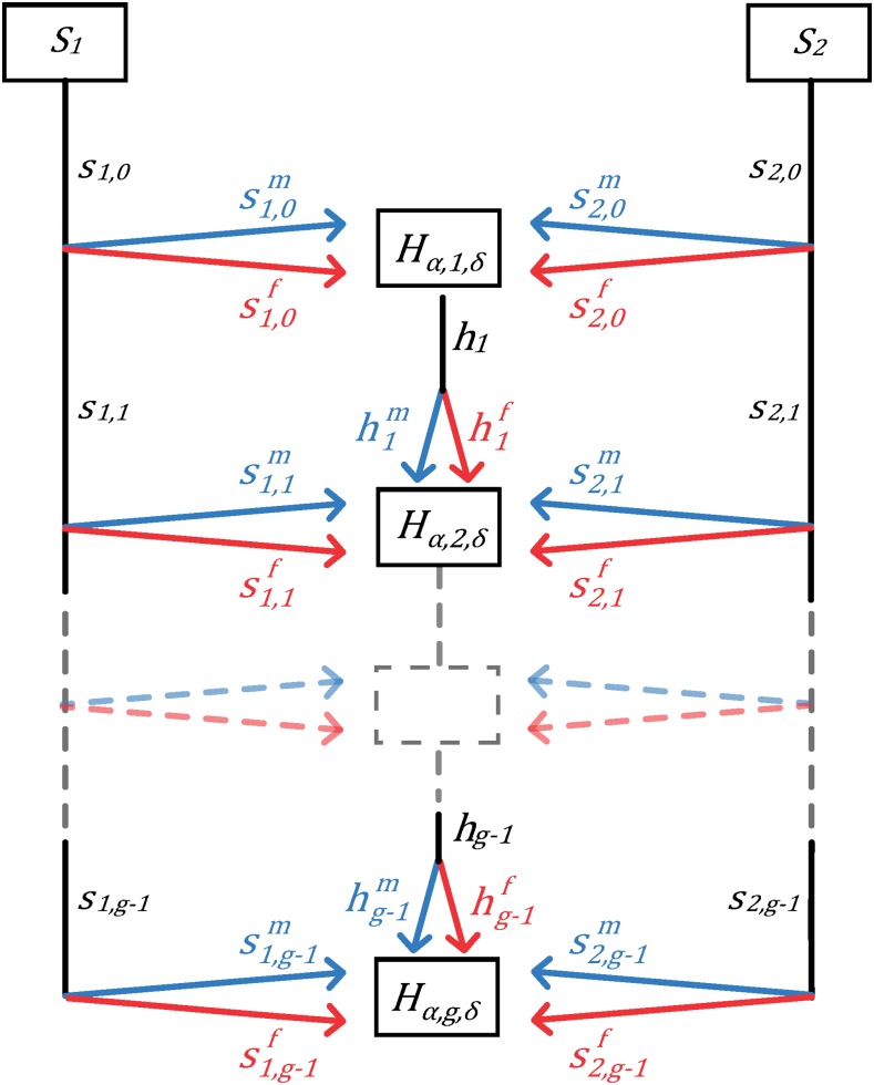
We demonstrate this surprising result through an extension of a mechanistic model for the admixture history of a hybrid population. In a diploid autosomal framework, Verdu and Rosenberg (2011) examined contributions of multiple source populations that varied through time, without considering sex specificity. Here, expanding on the model of Verdu and Rosenberg (2011), we develop a model that mechanistically considers sex-specific admixture histories in which multiple source populations contribute to the admixed population, potentially with varying female and male contributions across generations (Figure 1). In an admixed population descended from two source populations, we derive the moments of the distribution of the fraction of autosomal admixture from a specific source population, as a function of sex-specific admixture parameters and time. We analyze the behavior of the model, considering admixture processes that are constant in time, and we show that the moments contain information about the sex bias.

Figure 1.

Schematic of the mechanistic model of admixture. Two source populations, S₁ and S₂, contribute both males and females to the next generation of the hybrid population H, potentially with time-varying proportions. The fractional contributions of the source populations and the hybrid population to the next generation g are $s_{1,g},s_{2,g}$, and h_g, respectively. Sex-specific contributions from the populations are $s_{1,g}^{\text{f}}$, $s_{2,g}^{\text{f}}$, and $s_{1,g}^{\text{m}}$, $s_{2,g}^{\text{m}},$ for females and males respectively. H_α,g,δ represents the fraction of admixture from source population α ∈ {1, 2} in generation g for a random individual of sex δ ∈ {f, m} in population H.

The Model

Several studies have described mechanistic models of admixture (Chakraborty and Weiss 1988; Long 1991; Ewens and Spielman 1995; Guo et al. 2005; Verdu and Rosenberg 2011; Gravel 2012; Jin et al. 2014). We follow the notation and style of the model of Verdu and Rosenberg (2011), studying a hybrid population, H, which consists of immigrant individuals from M isolated source populations and hybrid individuals who have ancestors from two or more source populations. The source populations are labeled S_α, for α from 1 to M. We focus on the case of M = 2.

We define the parameters s_α,g−1 and h_g−1 as the contributions from source populations S_α and H, respectively, to the gene pool of the hybrid population H at the next generation, g. That is, for a random individual at generation g, the probabilities that a randomly chosen parent of the individual derives from S_α and H are s_α,g−1 and h_g−1, respectively. We define the sex-specific parameter $s_{\alpha ,g-1}^{\delta }$, for δ ∈ {f, m}, as the probability that the type-δ parent of a randomly chosen individual from the hybrid population at generation g is from source population S_α. Similarly, $h_{g-1}^{\delta }$ is the probability that the type-δ parent of a randomly chosen individual in H at generation g is from H itself. We consider a two-sex model, using f for female and m for male. Because each individual has one parent of each type, female and male, we have

$$s_{\alpha ,g-1}=\left(s_{\alpha ,g-1}^{\text{f}}+s_{\alpha ,g-1}^{\text{m}}\right)/2,$$ (1)

$$h_{g-1}=\left(h_{g-1}^{\text{f}}+h_{g-1}^{\text{m}}\right)/2.$$ (2)

The contributions to the next generation of the three source populations (S₁, S₂, H) sum to one:

$$s_{1,g-1}+s_{2,g-1}+h_{g-1}=1.$$ (3)

Similarly, the female and male contributions to the next generation separately sum to one,

$$s_{1,g-1}^{\text{f}}+s_{2,g-1}^{\text{f}}+h_{g-1}^{\text{f}}=s_{1,g-1}^{\text{m}}+s_{2,g-1}^{\text{m}}+h_{g-1}^{\text{m}}=1.$$ (4)

At the first generation, g = 1, the hybrid population has not previously existed; therefore,

$$h_0=h_0^{\text{f}}=h_0^{\text{m}}=0,$$ (5)

$$s_{1,0}+s_{2,0}=s_{1,0}^{\text{f}}+s_{2,0}^{\text{f}}=s_{1,0}^{\text{m}}+s_{2,0}^{\text{m}}=1.$$ (6)

The first generation has two independent parameters, $s_{1,0}^{\text{f}}$ and $s_{1,0}^{\text{m}}$. Each subsequent generation contributes four independent parameters $\left(s_{1,g-1}^{\text{f}},s_{2,g-1}^{\text{f}},s_{1,g-1}^{\text{m}},s_{2,g-1}^{\text{m}}\right)$, and considering g generations, there are 4g − 2 independent parameters. The model is discrete in time with nonoverlapping generations. As in Verdu and Rosenberg (2011), our deterministic treatment amounts to an assumption of infinite population size.

Our model enables us to consider complex sex-biased admixture processes by allowing uneven sex-specific contributions from each source population at each generation. It reduces to the Verdu and Rosenberg (2011) model when the sex-specific contributions are equal within source populations, that is, if for each g, $s_{1,g-1}^{\text{f}}=s_{1,g-1}^{\text{m}}$ and $s_{2,g-1}^{\text{f}}=s_{2,g-1}^{\text{m}}$. We perform similar computations to those of Verdu and Rosenberg (2011), finding that in certain cases, our results reduce to those obtained when sex specificity is not considered.

We let L be a random variable indicating the source populations of the parents of a random individual from the hybrid population, H. L takes its values from the set of all possible ordered parental combinations, {S₁S₁, S₁H, S₁S₂, HS₁, HH, HS₂, S₂S₁, S₂H, S₂S₂}, listing the female parent first. We assume random mating in the hybrid population at each generation, so that the probability that an offspring has a particular pair of source populations for his or her parents is simply the product of separate probabilities associated with the female and male parents (Table 1).

Table 1. Probabilities that an individual from the hybrid population at generation g has one of nine possible sets of parents from S₁, S₂, or H, assuming random mating.

Case	Female parent’s population	Male parent’s population	Probability
1	S1	S1	$s_{1,g-1}^{\text{f}}{s}_{1,g-1}^{\text{m}}$
2	S1	H	$s_{1,g-1}^{\text{f}}{h}_{g-1}^{\text{m}}$
3	S1	S2	$s_{1,g-1}^{\text{f}}{s}_{2,g-1}^{\text{m}}$
4	H	S1	$h_{g-1}^{\text{f}}{s}_{1,g-1}^{\text{m}}$
5	H	H	$h_{g-1}^{\text{f}}{s}_{g-1}^{\text{m}}$
6	H	S2	$h_{g-1}^{\text{f}}{s}_{2,g-1}^{\text{m}}$
7	S2	S1	$s_{2,g-1}^{\text{f}}{s}_{1,g-1}^{\text{m}}$
8	S2	H	$s_{2,g-1}^{\text{f}}{h}_{g-1}^{\text{m}}$
9	S2	S2	$s_{2,g-1}^{\text{f}}{s}_{2,g-1}^{\text{m}}$

The parameter $s_{\alpha ,g}^{\delta }$ is the probability that the parent of sex δ for a randomly chosen individual from the hybrid population, at generation g, is from the source population α. Similarly, the probability that this parent is from H is $h_g^{\delta }$.

We define the fraction of admixture, the random variable H_α,g,δ, as the probability that an autosomal genetic locus in a random individual of sex δ from the hybrid population in generation g ultimately originates from source population α. The sex-specific fractions of admixture are related to the total fraction of admixture H_α,g from source population α in generation g by H_α,g = (H_α,g,f + H_α,g,m)/2.

Under the model, we derive expressions for the moments of the fraction of admixture. Autosomal DNA is inherited non-sex-specifically and from both parents; therefore, female and male offspring have identical distributions of admixture, and H_α,g,f and H_α,g,m are identically distributed. Each of these quantities depends on both the female and male fractions of admixture in the previous generation, but conditional on the previous generation (that is, on H_α,g−1,f and H_α,g−1,m), they are independent. For our two-population model, we consider the non-sex-specific fraction of admixture, H_1,g,δ, treating δ here as representing either f or m, but retaining the same meaning through a calculation. The quantity H_1,g,δ depends on both sex-specific fractions of admixture from the previous generation, H_1,g−1,f and H_1,g−1,m.

Distribution of the Admixture Fraction from a Specific Source

The definition of the model parameters and the values from Table 1 allow us to write a recursion relation for the fraction of admixture from source population 1 for a random individual of sex δ from the hybrid population at generation g, or H_1,g,δ. For the first generation, g = 1, we have

$$H_{1,1,\delta }=\{\begin{array}{cc}1& \text{if}\hspace{0.17em}L=S_1{S}_1,\text{with}\hspace{0.17em}\mathrm{\mathbb{P}}\left[L=S_1{S}_1\right]=s_{1,0}^{\mathrm{f}}{s}_{1,0}^{\mathrm{m}}\\ \frac{1}{2}& \text{if}\hspace{0.17em}L=S_1{S}_2,\text{with}\hspace{0.17em}\mathrm{\mathbb{P}}\left[L=S_1{S}_2\right]=s_{1,0}^{\mathrm{f}}{s}_{2,0}^{\mathrm{m}}\\ \frac{1}{2}& \text{if}\hspace{0.17em}L=S_2{S}_1,\text{with}\hspace{0.17em}\mathrm{\mathbb{P}}\left[L=S_2{S}_1\right]=s_{2,0}^{\mathrm{f}}{s}_{1,0}^{\mathrm{m}}\\ 0& \text{if}\hspace{0.17em}L=S_2{S}_2,\text{with}\hspace{0.17em}\mathrm{\mathbb{P}}\left[L=S_2{S}_2\right]=s_{2,0}^{\mathrm{f}}{s}_{2,0}^{\mathrm{m}}.\end{array}$$ (7)

For all subsequent generations, g ≥ 2, we have

$$H_{1,g,\delta }=\{\begin{array}{ll}1\hfill & \text{if}\hspace{0.17em}L=S_1{S}_1,\text{with}\hspace{0.17em}\mathrm{\mathbb{P}}\left[L=S_1{S}_1\right]=s_{1,g-1}^{\mathrm{f}}{s}_{1,g-1}^{\mathrm{m}}\hfill \\ \frac{1+H_{1,g-1,m}}{2}\hfill & \text{if}\hspace{0.17em}L=S_{1}H,\text{with\hspace{0.17em}}\mathrm{\mathbb{P}}\left[L=S_{1}H\right]=s_{1,g-1}^{\mathrm{f}}{h}_{g-1}^{\mathrm{m}}\hfill \\ \frac{1}{2}\hfill & \text{if}\hspace{0.17em}L=S_1{S}_2,\text{with\hspace{0.17em}}\mathrm{\mathbb{P}}\left[L=S_1{S}_2\right]=s_{1,g-1}^{\mathrm{f}}{s}_{2,g-1}^{\mathrm{m}}\hfill \\ \frac{1+H_{1,g-1,f}}{2}\hfill & \text{if}\hspace{0.17em}L=H{S}_1,\text{with\hspace{0.17em}}\mathrm{\mathbb{P}}\left[L=H{S}_1\right]=h_{g-1}^{\mathrm{f}}{s}_{1,g-1}^{\mathrm{m}}\hfill \\ \frac{H_{1,g-1,f}+H_{1,g-1,m}}{2}\hfill & \text{if}\hspace{0.17em}L=HH,\text{with\hspace{0.17em}}\mathrm{\mathbb{P}}\left[L=HH\right]=h_{g-1}^{\mathrm{f}}{h}_{g-1}^{\mathrm{m}}\hfill \\ \frac{H_{1,g-1,f}}{2}\hfill & \text{if}\hspace{0.17em}L=H{S}_2,\text{with\hspace{0.17em}}\mathrm{\mathbb{P}}\left[L=H{S}_2\right]=h_{g-1}^{\mathrm{f}}{s}_{2,g-1}^{\mathrm{m}}\hfill \\ \frac{1}{2}\hfill & \text{if}\hspace{0.17em}L=S_2{S}_1,\text{with\hspace{0.17em}}\mathrm{\mathbb{P}}\left[L=S_2{S}_1\right]=s_{2,g-1}^{\mathrm{f}}{s}_{1,g-1}^{\mathrm{m}}\hfill \\ \frac{H_{1,g-1,m}}{2}\hfill & \text{if}\hspace{0.17em}L=S_{2}H,\text{with\hspace{0.17em}}\mathrm{\mathbb{P}}\left[L=S_{2}H\right]=s_{2,g-1}^{\mathrm{f}}{h}_{g-1}^{\mathrm{m}}\hfill \\ 0\hfill & \text{if}\hspace{0.17em}L=S_2{S}_2,\text{with\hspace{0.17em}}\mathrm{\mathbb{P}}\left[L=S_2{S}_2\right]=s_{2,g-1}^{\mathrm{f}}{s}_{2,g-1}^{\mathrm{m}}.\hfill \end{array}$$ (8)

Using Equations 7 and 8, we can analyze the distribution of the fraction of admixture as a function of the time g and the parameters $s_{1,g}^{\text{f}},s_{1,g}^{\text{m}},s_{2,g}^{\text{f}},s_{2,g}^{\text{m}}$. Under our model, H_1,g,δ takes its values in Q_g = {0, 1/2^g, …, 1−1/2^g, 1}. Therefore, using Equations 7 and 8, and recalling that H_1,g,f and H_1,g,m are identically distributed, for a value q in the set Q_g, we can compute the probability ℙ(H_1,g,δ = q) that a random individual from the hybrid population at generation g has admixture fraction q. For g = 1, $Q_1=\left\{0,\frac{1}{2},1\right\}$, and

$$\mathrm{\mathbb{P}}\left(H_{1,1,\delta }=q\right)=\{\begin{array}{ll}{s}_{1,0}^{\text{f}}{s}_{1,0}^{\text{m}}\hfill & \text{if}\hspace{0.17em}q=1\hfill \\ s_{1,0}^{\text{f}}{s}_{2,0}^{\text{m}}+s_{2,0}^{\text{f}}{s}_{1,0}^{\text{m}}\hfill & \text{if}\hspace{0.17em}q=\frac{1}{2}\hfill \\ s_{2,0}^{\text{f}}{s}_{2,0}^{\text{m}}\hfill & \text{if}\hspace{0.17em}q=0.\hfill \end{array}$$ (9)

For all subsequent generations, g ≥ 2, for q in Q_g,

$$\begin{array}{c}\mathrm{\mathbb{P}}\left(H_{1,g,\delta }=q\right)=h_{g-1}^{\text{f}}{h}_{g-1}^{\text{m}}{\displaystyle \sum _{r=0}^{2^{g-1}}\left[\mathrm{\mathbb{P}}\left(H_{1,g-1,{\delta }_1}=\frac{r}{2^{g-1}}\right)\mathrm{\mathbb{P}}\left(H_{1,g-1,{\delta }_2}=\frac{2^{g}q-r}{2^{g-1}}\right)\right]}\\ +\left(s_{1,g-1}^{\text{f}}{h}_{g-1}^{\text{m}}+h_{g-1}^{\text{f}}{s}_{1,g-1}^{\text{m}}\right)\mathrm{\mathbb{P}}\left(H_{1,g-1,\delta }=2q-1\right)\\ +\left(s_{2,g-1}^{\text{f}}{h}_{g-1}^{\text{m}}+h_{g-1}^{\text{f}}{s}_{2,g-1}^{\text{m}}\right)\mathrm{\mathbb{P}}\left(H_{1,g-1,\delta }=2q\right)+I_g\left(q\right).\end{array}$$ (10)

The function I_g is defined for all values of q in Q_g and is equal to

$$I_g\left(q\right)=\{\begin{array}{ll}{s}_{1,g-1}^{\text{f}}{s}_{1,g-1}^{\text{m}}\hfill & \text{if}\hspace{0.17em}q=1\hfill \\ s_{1,g-1}^{\text{f}}{s}_{2,g-1}^{\text{m}}+s_{2,g-1}^{\text{f}}{s}_{1,g-1}^{\text{m}}\hfill & \text{if}\hspace{0.17em}q=\frac{1}{2}\hfill \\ s_{2,g-1}^{\text{f}}{s}_{2,g-1}^{\text{m}}\hfill & \text{if}\hspace{0.17em}q=0\hfill \\ 0\hfill & \text{otherwise}.\hfill \end{array}$$ (11)

In Equation 10, we calculate the probability distribution of H_1,g,δ by taking a sum over all possible parental pairings at the previous generation that would lead to an admixture fraction q at generation g. Only three values of q allow for a history without a single hybrid ancestor—q = 0, $q=\frac{1}{2}$, and q = 1—producing the terms in Equation 11. When there is no sex bias and $s_{1,g-1}^{\text{f}}=s_{1,g-1}^{\text{m}},h_{g-1}^{\text{f}}=h_{g-1}^{\text{m}},$ and $s_{2,g-1}^{\text{f}}=s_{2,g-1}^{\text{m}}$, Equations 9–11 reduce to the corresponding Equations 3–5 from Verdu and Rosenberg (2011).

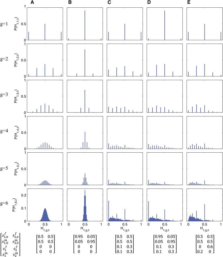
Equations 9–11 can be used to analyze the behavior of the distribution of H_1,g−1,δ over time. In Figure 2, we consider constant admixture processes after the founding of the hybrid population ($s_{\alpha ,g}^{\delta }=s_{\alpha }^{\delta }$ for each α ∈ {1, 2}, δ ∈ {f, m}, and g ≥ 1), plotting ℙ(H_1,g,δ) for the first six generations, as computed recursively using Equation 10. In Figure 2, A and B, we consider a hybrid population founded with equal contributions from source populations S₁ and S₂, but with no further contributions after g = 1. In both of these cases, the distribution of the autosomal admixture fraction contracts around the mean of $\frac{1}{2}$. However, whereas Figure 2A has equal contributions from each sex in the founding generation, Figure 2B has a large initial sex bias. We see that the width of the distribution is smaller with the sex-biased contributions, despite equality of the total contributions s_1,0 and s_2,0.

Figure 2.

Probability distribution of the fraction of admixture from source population S₁, $\mathrm{\mathbb{P}}\left(H_{1,g,\delta }\right)$, for a random individual from the hybrid population for the first six generations (Equations 9–11). Each column (A, B, C, D, E) corresponds to a specified admixture scenario, with constant contributions from the source populations over time after founding ($s_{\alpha ,g}^{\delta }=s_{\alpha }^{\delta }$ for each α ∈ {1, 2}, δ ∈ {f, m}, and g ≥ 2).

In Figures 2, C–E, we consider admixture scenarios in which the founding of the hybrid population is followed by constant contributions from the source populations over time, s₁ = 0.1 and s₂ = 0.3. Because the two source populations contribute after the founding, the distribution does not contract around the mean as in Figures 2, A and B. Also, because the total contributions from S₁ and S₂ are unequal, the distribution of H_1,g,δ is no longer symmetrical. Rather, because the contribution from S₂ is greater, the distribution is shifted toward zero.

Figures 2, C and D, have the same continuing contributions for g ≥ 2, with no sex bias in the founding generation for Figure 2C, and a large initial sex bias for Figure 2D. Despite different founding contributions, Figures 2, C and D, have similar distributions of H_1,g,δ after a few generations. In Figure 2E, the hybrid population is founded without a sex bias and with equal contributions from the two source populations. The total contributions s₁ and s₂ are the same as in Figures 2, C and D, but unlike in Figures 2, C and D, the continuing contributions are sex biased, with $s_1^{\text{f}}\ne s_1^{\text{m}}$ and $s_2^{\text{f}}\ne s_2^{\text{m}}$. Even with s₁ and s₂ held constant, the distribution of H_1,g,δ depends on the $s_{\alpha }^{\delta }$. Notably, the probability of H_1,6,δ = 0 drops from 0.157 in Figure 2C to 0.000 in Figure 2E. Similarly, ℙ(H_1,6,δ = 1) drops to zero in Figure 2E as well. With these reductions at the extremes, we see a rise in the probability of intermediate values for H_1,g,δ.

Expectation of the Fraction of Admixture

Using the law of total expectation, we write the expectation of the fraction of admixture from source population 1 for a random individual of sex δ in population H at generation g as a function of conditional expectations for all possible pairs of parents L,

$$\mathbb{E}\left[H_{1,g,\delta }\right]={\mathbb{E}}_L\left[\mathbb{E}\left[H_{1,g,\delta }|L\right]\right]={\displaystyle \sum _{\ell \in \left\{\begin{array}{c}{S}_1{S}_1\\ S_{1}H\\ S_1{S}_2\\ H{S}_1\\ HH\\ H{S}_2\\ S_2{S}_1\\ S_{2}H\\ S_2{S}_2\end{array}\right\}}\mathrm{\mathbb{P}}\left(L=\ell \right)\mathbb{E}\left[H_{1,g,\delta }|L=\ell \right]}.$$ (12)

We can simplify this recursion relation. For g = 1,

$$\begin{array}{c}\mathbb{E}\left[H_{1,1,\delta }\right]=\mathrm{\mathbb{P}}\left(L=S_1{S}_1\right)\mathbb{E}\left[H_{1,1,\delta }|L=S_1{S}_1\right]\\ +\mathrm{\mathbb{P}}\left(L=S_1{S}_2\right)\mathbb{E}\left[H_{1,1,\delta }|L=S_1{S}_2\right]\\ +\mathrm{\mathbb{P}}\left(L=S_2{S}_1\right)\mathbb{E}\left[H_{1,1,\delta }|L=S_2{S}_1\right]\\ +\mathrm{\mathbb{P}}\left(L=S_2{S}_2\right)\mathbb{E}\left[H_{1,1,\delta }|L=S_2{S}_2\right].\end{array}$$ (13)

For all subsequent generations, g ≥ 2, we have

$$\begin{array}{c}\mathbb{E}\left[H_{1,g,\delta }\right]=\mathrm{\mathbb{P}}\left(L=S_1{S}_1\right)\mathbb{E}\left[H_{1,g,\delta }|L=S_1{S}_1\right]\\ +\mathrm{\mathbb{P}}\left(L=S_{1}H\right)\mathbb{E}\left[H_{1,g,\delta }|L=S_{1}H\right]\\ +\mathrm{\mathbb{P}}\left(L=S_1{S}_2\right)\mathbb{E}\left[H_{1,g,\delta }|L=S_1{S}_2\right]\\ +\mathrm{\mathbb{P}}\left(L=H{S}_1\right)\mathbb{E}\left[H_{1,g,\delta }|L=H{S}_1\right]\\ +\mathrm{\mathbb{P}}\left(L=HH\right)\mathbb{E}\left[H_{1,g,\delta }|L=HH\right]\\ +\mathrm{\mathbb{P}}\left(L=H{S}_2\right)\mathbb{E}\left[H_{1,g,\delta }|L=H{S}_2\right]\\ +\mathrm{\mathbb{P}}\left(L=S_2{S}_1\right)\mathbb{E}\left[H_{1,g,\delta }|L=S_2{S}_1\right]\\ +\mathrm{\mathbb{P}}\left(L=S_{2}H\right)\mathbb{E}\left[H_{1,g,\delta }|L=S_{2}H\right]\\ +\mathrm{\mathbb{P}}\left(L=S_2{S}_2\right)\mathbb{E}\left[H_{1,g,\delta }|L=S_2{S}_2\right].\end{array}$$ (14)

Using Equations 7 and 8, for the first generation, g = 1, we have

$$\begin{array}{c}\mathbb{E}\left[H_{1,1,\delta }\right]=s_{1,0}^{\text{f}}{s}_{1,0}^{\text{m}}\mathbb{E}\left[1\right]\\ +\left(s_{1,0}^{\text{f}}{s}_{2,0}^{\text{m}}+s_{2,0}^{\text{f}}{s}_{1,0}^{\text{m}}\right)\mathbb{E}\left[\frac{1}{2}\right]\\ +s_{2,0}^{\text{f}}{s}_{2,0}^{\text{m}}\mathbb{E}\left[0\right].\end{array}$$ (15)

For all subsequent generations, g ≥ 2, we have

$$\begin{array}{c}\mathbb{E}\left[H_{1,g,\delta }\right]=s_{1,g-1}^{\text{f}}{s}_{1,g-1}^{\text{m}}\mathbb{E}\left[1\right]\\ +s_{1,g-1}^{\text{f}}{h}_{g-1}^{\text{m}}\mathbb{E}\left[\frac{1+H_{1,g-1,m}}{2}\right]+h_{g-1}^{\text{f}}{s}_{1,g-1}^{\text{m}}\mathbb{E}\left[\frac{1+H_{1,g-1,f}}{2}\right]\\ +\left(s_{1,g-1}^{\text{f}}{s}_{2,g-1}^{\text{m}}+s_{2,g-1}^{\text{f}}{s}_{1,g-1}^{\text{m}}\right)\mathbb{E}\left[\frac{1}{2}\right]\\ +h_{g-1}^{\text{f}}{h}_{g-1}^{\text{m}}\mathbb{E}\left[\frac{H_{1,g-1,f}+H_{1,g-1,m}}{2}\right]\\ +s_{2,g-1}^{\text{f}}{h}_{g-1}^{\text{m}}\mathbb{E}\left[\frac{H_{1,g-1,m}}{2}\right]+h_{g-1}^{\text{f}}{s}_{2,g-1}^{\text{m}}\mathbb{E}\left[\frac{H_{1,g-1,f}}{2}\right]\\ +s_{2,g-1}^{\text{f}}{s}_{2,g-1}^{\text{m}}\mathbb{E}\left[0\right].\end{array}$$ (16)

Recalling Equations 1, 2, and 4, we can simplify the expectation of the fraction of admixture in a random individual of sex δ from the hybrid population. For g = 1, Equation 15 gives

$$\mathbb{E}\left[H_{1,1,\delta }\right]=s_{1,0},$$ (17)

the same expression found by Verdu and Rosenberg (2011, Equation 10). For g ≥ 2, by Equation 16,

$$\mathbb{E}\left[H_{1,g,\delta }\right]=s_{1,g-1}+\frac{1}{2}\left(h_{g-1}^{\text{f}}\mathbb{E}\left[H_{1,g-1,f}\right]+h_{g-1}^{\text{m}}\mathbb{E}\left[H_{1,g-1,m}\right]\right).$$ (18)

Because H_1,g,f and H_1,g,m are identically distributed, recalling Equation 2, we can simplify the expectation using $\mathbb{E}\left[H_{1,g,f}\right]=\mathbb{E}\left[H_{1,g,m}\right]=\mathbb{E}\left[H_{1,g,\delta }\right]$, where δ is left as an unspecified sex (f or m). For g ≥ 2, the expectation of the fraction of admixture from source population 1 is

$$\mathbb{E}\left[H_{1,g,\delta }\right]=s_{1,g-1}+h_{g-1}\mathbb{E}\left[H_{1,g-1,\delta }\right].$$ (19)

We see in Equations 17 and 19 that the expectation of the fraction of admixture for a random individual of sex δ from the hybrid population at generation g, $\mathbb{E}\left[H_{1,g,\delta }\right]$, depends on the total contributions of the source populations (S₁, S₂, H) at each generation, s_1,g−1 and h_g−1, and not on the sex-specific parameters, $s_{1,g-1}^{\text{f}}$, $s_{1,g-1}^{\text{m}}$, $h_{g-1}^{\text{f}}$, and $h_{g-1}^{\text{m}}$. This recursion (Equations 17 and 19) is the same as in the non-sex-specific model of Verdu and Rosenberg (2011, Equations 10 and 11).

Higher Moments of the Fraction of Admixture

We can write a general recursion for the higher moments of the admixture fraction from population S₁ in a randomly chosen individual of sex δ from the hybrid population. For k ≥ 1, in generation g = 1,

$$H_{1,1,\delta }^k=\{\begin{array}{cc}{1}^k& \text{if}\hspace{0.5em}L=S_1{S}_1,\text{with}\hspace{0.5em}\mathrm{\mathbb{P}}\left[L=S_1{S}_1\right]=s_{1,0}^{\text{f}}{s}_{1,0}^{\text{m}}\\ {\left(\frac{1}{2}\right)}^k& \text{if}\hspace{0.5em}L=S_1{S}_2,\text{with}\hspace{0.5em}\mathrm{\mathbb{P}}\left[L=S_1{S}_2\right]=s_{1,0}^{\text{f}}{s}_{2,0}^{\text{m}}\\ {\left(\frac{1}{2}\right)}^k& \text{if}\hspace{0.5em}L=S_2{S}_1,\text{with}\hspace{0.5em}\mathrm{\mathbb{P}}\left[L=S_2{S}_1\right]=s_{2,0}^{\text{f}}{s}_{1,0}^{\text{m}}\\ 0^k& \text{if}\hspace{0.5em}L=S_2{S}_2,\text{with}\hspace{0.5em}\mathrm{\mathbb{P}}\left[L=S_2{S}_2\right]=s_{2,0}^{\text{f}}{s}_{2,0}^{\text{m}}.\end{array}$$ (20)

For all subsequent generations, g ≥ 2,

$$H_{1,g,\delta }^k=\{\begin{array}{ll}{1}^k\hfill & \text{if}\hspace{0.5em}L=S_1{S}_1,\text{with}\hspace{0.5em}\mathrm{\mathbb{P}}\left[L=S_1{S}_1\right]=s_{1,g-1}^{\text{f}}{s}_{1,g-1}^{\text{m}}\hfill \\ {\left(\frac{1+H_{1,g-1,m}}{2}\right)}^k\hfill & \text{if}\hspace{0.5em}L=S_{1}H,\text{with}\hspace{0.5em}\mathrm{\mathbb{P}}\left[L=S_{1}H\right]=s_{1,g-1}^{\text{f}}{h}_{g-1}^{\text{m}}\hfill \\ {\left(\frac{1}{2}\right)}^k\hfill & \text{if}\hspace{0.5em}L=S_1{S}_2,\text{with}\hspace{0.5em}\mathrm{\mathbb{P}}\left[L=S_1{S}_2\right]=s_{1,g-1}^{\text{f}}{s}_{2,g-1}^{\text{m}}\hfill \\ {\left(\frac{1+H_{1,g-1,f}}{2}\right)}^k\hfill & \text{if}\hspace{0.5em}L=H{S}_1,\text{with}\hspace{0.5em}\mathrm{\mathbb{P}}\left[L=H{S}_1\right]=h_{g-1}^{\text{f}}{s}_{1,g-1}^{\text{m}}\hfill \\ {\left(\frac{H_{1,g-1,f}+H_{1,g-1,m}}{2}\right)}^k\hfill & \text{if}\hspace{0.5em}L=HH,\text{with}\hspace{0.5em}\mathrm{\mathbb{P}}\left[L=H{S}_1\right]=h_{g-1}^{\text{f}}{h}_{g-1}^{\text{m}}\hfill \\ {\left(\frac{H_{1,g-1,f}}{2}\right)}^k\hfill & \text{if}\hspace{0.5em}L=H{S}_2,\text{with}\hspace{0.5em}\mathrm{\mathbb{P}}\left[L=H{S}_2\right]=h_{g-1}^{\text{f}}{s}_{2,g-1}^{\text{m}}\hfill \\ {\left(\frac{1}{2}\right)}^k\hfill & \text{if}\hspace{0.5em}L=S_2{S}_1,\text{with}\hspace{0.5em}\mathrm{\mathbb{P}}\left[L=S_2{S}_1\right]=s_{2,g-1}^{\text{f}}{s}_{1,g-1}^{\text{m}}\hfill \\ {\left(\frac{H_{1,g-1,m}}{2}\right)}^k\hfill & \text{if}\hspace{0.5em}L=S_{2}H,\text{with}\hspace{0.5em}\mathrm{\mathbb{P}}\left[L=S_{2}H\right]=s_{2,g-1}^{\text{f}}{h}_{g-1}^{\text{m}}\hfill \\ 0^k\hfill & \text{if}\hspace{0.5em}L=S_2{S}_2,\text{with}\hspace{0.5em}\mathrm{\mathbb{P}}[L=S_2{S}_2]=s_{2,g-1}^{\text{f}}{s}_{2,g-1}^{\text{m}}.\hfill \end{array}$$ (21)

As in the case of k = 1, we use the law of total expectation to write a recursion for higher moments of the distribution of the fraction of admixture for all k ≥ 1. Using the values for the recursion for the fraction of admixture, Equations 7 and 8, in the first generation, g = 1, we have

$$\begin{array}{c}\mathbb{E}\left[H_{1,1,\delta }^k\right]=s_{1,0}^{\text{f}}{s}_{1,0}^{\text{m}}\mathbb{E}\left[1^k\right]\\ +\left(s_{1,0}^{\text{f}}{s}_{2,0}^{\text{m}}+s_{2,0}^{\text{f}}{s}_{1,0}^{\text{m}}\right)\mathbb{E}\left[{\left(\frac{1}{2}\right)}^k\right]\\ +s_{2,0}^{\text{f}}{s}_{2,0}^{\text{m}}\mathbb{E}[0^k].\end{array}$$ (22)

For g ≥ 2, we have

$$\begin{array}{c}\mathbb{E}\left[H_{1,g,\delta }^k\right]=s_{1,g-1}^{\text{f}}{s}_{1,g-1}^{\text{m}}\mathbb{E}\left[1^k\right]\\ +s_{1,g-1}^{\text{f}}{h}_{g-1}^{\text{m}}\mathbb{E}\left[{\left(\frac{1+H_{1,g-1,m}}{2}\right)}^k\right]+h_{g-1}^{\text{f}}{s}_{1,g-1}^{\text{m}}\mathbb{E}\left[{\left(\frac{1+H_{1,g-1,f}}{2}\right)}^k\right]\\ +\left(s_{1,g-1}^{\text{f}}{s}_{2,g-1}^{\text{m}}+s_{2,g-1}^{\text{f}}{s}_{1,g-1}^{\text{m}}\right)\mathbb{E}\left[{\left(\frac{1}{2}\right)}^k\right]\\ +h_{g-1}^{\text{f}}{h}_{g-1}^{\text{m}}\mathbb{E}\left[{\left(\frac{H_{1,g-1,f}+H_{1,g-1,m}}{2}\right)}^k\right]\\ +s_{2,g-1}^{\text{f}}{h}_{g-1}^{\text{m}}\mathbb{E}\left[{\left(\frac{H_{1,g-1,m}}{2}\right)}^k\right]+h_{g-1}^{\text{f}}{s}_{2,g-1}^{\text{m}}\mathbb{E}\left[{\left(\frac{H_{1,g-1,f}}{2}\right)}^k\right]\\ +s_{2,g-1}^{\text{f}}{s}_{2,g-1}^{\text{m}}\mathbb{E}\left[0^k\right].\end{array}$$ (23)

Recalling Equation 3 and noting that h₀ = 0, we use the binomial theorem to simplify the recursion for the moments of H_1,g,δ. For g = 1, we have

$$\mathbb{E}\left[H_{1,1,\delta }^k\right]=s_{1,0}^{\text{f}}{s}_{1,0}^{\text{m}}+\frac{s_{1,0}^{\text{f}}{s}_{2,0}^{\text{m}}+s_{2,0}^{\text{f}}{s}_{1,0}^{\text{m}}}{2^k}.$$ (24)

For g ≥ 2, we have

$$\begin{array}{c}\mathbb{E}\left[H_{1,g,\delta }^k\right]=s_{1,g-1}^{\text{f}}{s}_{1,g-1}^{\text{m}}+\frac{s_{1,g-1}^{\text{f}}{s}_{2,g-1}^{\text{m}}+s_{2,g-1}^{\text{f}}{s}_{1,g-1}^{\text{m}}}{2^k}\\ +\frac{s_{1,g-1}^{\text{f}}{h}_{g-1}^{\text{m}}}{2^k}\left({\displaystyle \sum _{i=0}^k\left(\begin{array}{c}k\\ i\end{array}\right)\mathbb{E}\left[H_{1,g-1,m}^i\right]}\right)\\ +\frac{h_{g-1}^{\text{f}}{s}_{1,g-1}^{\text{m}}}{2^k}\left({\displaystyle \sum _{i=0}^k\left(\begin{array}{c}k\\ i\end{array}\right)\mathbb{E}\left[H_{1,g-1,f}^i\right]}\right)\\ +\frac{h_{g-1}^{\text{f}}{h}_{g-1}^{\text{m}}}{2^k}\left({\displaystyle \sum _{i=0}^k\left(\begin{array}{c}k\\ i\end{array}\right)\mathbb{E}\left[H_{1,g-1,f}^{k-i}{H}_{1,g-1,m}^i\right]}\right)\\ +\frac{s_{2,g-1}^{\text{f}}{h}_{g-1}^{\text{m}}}{2^k}\mathbb{E}\left[H_{1,g-1,m}^k\right]+\frac{h_{g-1}^{\text{f}}{s}_{2,g-1}^{\text{m}}}{2^k}\mathbb{E}\left[H_{1,g-1,f}^k\right].\end{array}$$ (25)

Because H_1,g−1,f and H_1,g−1,m are conditionally independent given H_1,g−2,f and H_1,g−2,m, we can simplify the kth moment of the distribution of the fraction of admixture from S₁, for δ ∈ {f, m}, to give

$$\begin{array}{c}\mathbb{E}\left[H_{1,g,\delta }^k\right]=s_{1,g-1}^{\text{f}}{s}_{1,g-1}^{\text{m}}+\frac{s_{1,g-1}^{\text{f}}{s}_{2,g-1}^{\text{m}}+s_{2,g-1}^{\text{f}}{s}_{1,g-1}^{\text{m}}}{2^k}\\ +\frac{s_{1,g-1}^{\text{f}}{h}_{g-1}^{\text{m}}+h_{g-1}^{\text{f}}{s}_{1,g-1}^{\text{m}}}{2^k}\left({\displaystyle \sum _{i=0}^k\left(\begin{array}{c}k\\ i\end{array}\right)\mathbb{E}\left[H_{1,g-1,\delta }^i\right]}\right)\\ +\frac{h_{g-1}^{\text{f}}{h}_{g-1}^{\text{m}}}{2^k}\left({\displaystyle \sum _{i=0}^k\left(\begin{array}{c}k\\ i\end{array}\right)\mathbb{E}\left[H_{1,g-1,\delta }^{k-i}\right]\mathbb{E}\left[H_{1,g-1,\delta }^i\right]}\right)\\ +\frac{s_{2,g-1}^{\text{f}}{h}_{g-1}^{\text{m}}+h_{g-1}^{\text{f}}{s}_{2,g-1}^{\text{m}}}{2^k}\mathbb{E}\left[H_{1,g-1,\delta }^k\right].\end{array}$$ (26)

For k = 1, Equations 24 and 26 should produce the expectation that we have already derived for k = 1. For k = 1, using Equations 1, 2, and 4, Equation 24 gives

$$\mathbb{E}\left[H_{1,1,\delta }\right]=s_{1,0}^{\text{f}}{s}_{1,0}^{\text{m}}+\frac{s_{1,0}^{\text{f}}{s}_{2,0}^{\text{m}}+s_{2,0}^{\text{f}}{s}_{1,0}^{\text{m}}}{2}=s_{1,0},$$ (27)

which matches Equation 17. For g ≥ 2 and k = 1, Equation 26 gives

$$\begin{array}{c}\mathbb{E}\left[H_{1,g,\delta }\right]=s_{1,g-1}^{\text{f}}{s}_{1,g-1}^{\text{m}}+\frac{s_{1,g-1}^{\text{f}}{s}_{2,g-1}^{\text{m}}+s_{2,g-1}^{\text{f}}{s}_{1,g-1}^{\text{m}}+s_{1,g-1}^{\text{f}}{h}_{g-1}^{\text{m}}+h_{g-1}^{\text{f}}{s}_{1,g-1}^{\text{m}}}{2}\\ +\left(\frac{2h_{g-1}^{\text{f}}{h}_{g-1}^{\text{m}}+s_{1,g-1}^{\text{f}}{h}_{g-1}^{\text{m}}+h_{g-1}^{\text{f}}{s}_{1,g-1}^{\text{m}}+h_{g-1}^{\text{f}}{s}_{2,g-1}^{\text{m}}+s_{2,g-1}^{\text{f}}{h}_{g-1}^{\text{m}}}{2}\right)\mathbb{E}\left[H_{1,g-1,\delta }\right],\end{array}$$ (28)

which simplifies to match Equation 19. Finally, with equal contributions in each population from females and males, so that $s_{1,g-1}^{\text{f}}=s_{1,g-1}^{\text{m}}=s_{1,g-1}$ and $s_{2,g-1}^{\text{f}}=s_{2,g-1}^{\text{m}}=s_{2,g-1}$, Equations 24 and 26 reduce to Equations 16 and 17 from Verdu and Rosenberg (2011).

Variance of the Fraction of Admixture

When k = 2, Equations 24 and 26 produce a recursion for the second moment of H_1,g,δ. Recalling Equations 1–6, for g = 1, we have

$$\mathbb{E}\left[H_{1,1,\delta }^2\right]=\frac{s_{1,0}^{\text{f}}\left(1+s_{1,0}^{\text{m}}\right)+s_{1,0}^{\text{m}}\left(1+s_{1,0}^{\text{f}}\right)}{4}.$$ (29)

For g ≥ 2, we have

$$\begin{array}{c}\mathbb{E}\left[H_{1,g,\delta }^2\right]=s_{1,g-1}^{\text{f}}{s}_{1,g-1}^{\text{m}}+\frac{s_{1,g-1}^{\text{f}}{s}_{2,g-1}^{\text{m}}+s_{2,g-1}^{\text{f}}{s}_{1,g-1}^{\text{m}}}{4}\\ +\frac{s_{1,g-1}^{\text{f}}{h}_{g-1}^{\text{m}}}{4}\left(1+2\mathbb{E}\left[H_{1,g-1,m}\right]+\mathbb{E}\left[H_{1,g-1,m}^2\right]\right)\\ +\frac{h_{g-1}^{\text{f}}{s}_{1,g-1}^{\text{m}}}{4}\left(1+2\mathbb{E}\left[H_{1,g-1,f}\right]+\mathbb{E}\left[H_{1,g-1,f}^2\right]\right)\\ +\frac{h_{g-1}^{\text{f}}{h}_{g-1}^{\text{m}}}{4}\left(\mathbb{E}\left[H_{1,g-1,f}^2\right]+2\mathbb{E}\left[H_{1,g-1,f}\right]\mathbb{E}\left[H_{1,g-1,m}\right]+\mathbb{E}\left[H_{1,g-1,m}^2\right]\right)\\ +\frac{s_{2,g-1}^{\text{f}}{h}_{g-1}^{\text{m}}}{4}\mathbb{E}\left[H_{1,g-1,m}^2\right]+\frac{h_{g-1}^{\text{f}}{s}_{2,g-1}^{\text{m}}}{4}\mathbb{E}\left[H_{1,g-1,f}^2\right].\end{array}$$ (30)

Recalling that H_1,g,f and H_1,g,m are identically distributed, Equation 30 simplifies to give

$$\begin{array}{c}\mathbb{E}\left[H_{1,g,\delta }^2\right]=\frac{s_{1,g-1}^{\text{f}}\left(1+s_{1,g-1}^{\text{m}}\right)+s_{1,g-1}^{\text{m}}\left(1+s_{1,g-1}^{\text{f}}\right)}{4}\\ +\frac{s_{1,g-1}^{\text{f}}{h}_{g-1}^{\text{m}}+h_{g-1}^{\text{f}}{s}_{1,g-1}^{\text{m}}}{2}\mathbb{E}\left[H_{1,g-1,\delta }\right]+\frac{h_{g-1}^{\text{f}}{h}_{g-1}^{\text{m}}}{2}{\left(\mathbb{E}\left[H_{1,g-1,\delta }\right]\right)}^2\\ +\frac{h_{g-1}^{\text{f}}+h_{g-1}^{\text{m}}}{4}\mathbb{E}\left[H_{1,g-1,\delta }^2\right].\end{array}$$ (31)

Using the definition of the variance $\mathbb{V}\left[H_{1,g,\delta }\right]=\mathbb{E}\left[H_{1,g,\delta }^2\right]-{\left(\mathbb{E}\left[H_{1,g,\delta }\right]\right)}^2$, and Equations 17, 19, 29, and 31, for the first generation, for the variance of the fraction of admixture, we have

$$\mathbb{V}\left[H_{1,1,\delta }\right]=\frac{s_{1,0}^{\text{f}}\left(1-s_{1,0}^{\text{f}}\right)+s_{1,0}^{\text{m}}\left(1-s_{1,0}^{\text{m}}\right)}{4}.$$ (32)

For all subsequent generations, g ≥ 2, we have

$$\begin{array}{c}\mathbb{V}\left[H_{1,g,\delta }\right]=\frac{s_{1,g-1}^{\text{f}}\left(1-s_{1,g-1}^{\text{f}}\right)+s_{1,g-1}^{\text{m}}\left(1-s_{1,g-1}^{\text{m}}\right)}{4}-\frac{s_{1,g-1}^{\text{f}}{h}_{g-1}^{\text{f}}+s_{1,g-1}^{\text{m}}{h}_{g-1}^{\text{m}}}{2}\mathbb{E}\left[H_{1,g-1,\delta }\right]\\ +\frac{h_{g-1}^{\text{f}}\left(1-h_{g-1}^{\text{f}}\right)+h_{g-1}^{\text{m}}\left(1-h_{g-1}^{\text{m}}\right)}{4}{\left(\mathbb{E}\left[H_{1,g-1,\delta }\right]\right)}^2+\frac{h_{g-1}^{\text{f}}+h_{g-1}^{\text{m}}}{4}\mathbb{V}\left[H_{1,g-1,\delta }\right].\end{array}$$ (33)

With no sex bias, so that $s_{1,g}^{\text{f}}=s_{1,g}^{\text{m}}=s_{1,g}$ and $s_{2,g}^{\text{f}}=s_{2,g}^{\text{m}}=s_{2,g}$, Equations 32 and 33 are equivalent to Equations 22 and 23 from Verdu and Rosenberg (2011).

The recursion for the variance of the fraction of admixture of a random individual of sex δ from the hybrid population is dependent on the variance from the previous generation, the expectation from the previous generation, and its square. By contrast with the expectation, the variance of the fraction of admixture depends on the sex-specific contributions from the source populations.

Equations 32 and 33 are invariant with respect to an exchange of all variables corresponding to males (superscript m) with those corresponding with females (superscript f). Thus, although the variance is affected by the sex-specific admixture contributions, it does not identify the direction of the bias. Despite the dependence of the variance of the autosomal fraction of admixture on sex-specific contributions, under the model, the symmetry demonstrates that autosomal DNA alone does not identify which sex contributes more to the hybrid population from a given source population. This result is reasonable given the non-sex-specific inheritance pattern of autosomal DNA.

Special Case: A Single Admixture Event

Using the recursions in Equations 17, 19, 32, and 33, we can study specific cases in which the contributions are specified. We first consider the case in which the source populations S₁ and S₂ do not contribute to the hybrid population after its founding: $s_{1,g}^{\text{f}}=s_{1,g}^{\text{m}}=s_{2,g}^{\text{f}}=s_{2,g}^{\text{m}}=0$, and $h=\left(h_g^{\text{f}}+h_g^{\text{m}}\right)/2=1$, for all g ≥ 1. As before, at the first generation, the hybrid population is not yet formed, and h₀ = 0. Therefore, $s_{1,0}+s_{2,0}=s_{1,0}^{\text{f}}+s_{2,0}^{\text{f}}=s_{1,0}^{\text{m}}+s_{2,0}^{\text{m}}=1$.

Under this scenario, we can derive the exact expectation and variance of the autosomal fraction of admixture of a random individual from the hybrid population. In the case of a single admixture event, the expectation of the admixture fraction is equal to the expectation at the first generation, because the further contributions are all zero. Using Equation 19, s_1,g−1 = s_2,g−1 = 0 for all g ≥ 2. Therefore, from Equation 17, in the case of a single admixture event, for all g ≥ 1,

$$\mathbb{E}\left[H_{1,g,\delta }\right]=s_{1,0}.$$ (34)

The expectation of the autosomal fraction of admixture from S₁ is constant over time, and it depends on the total—not the sex-specific—contribution from the source population S₁. As in the general case in Equation 19, for a single admixture event, a sex bias does not affect the expectation. Because the source populations provide no further contributions after the founding generation, unlike in the general case, the mean admixture fraction does not change with time.

Using Equations 32 and 33, because $s_1^{\text{f}}=s_1^{\text{m}}=s_2^{\text{f}}=s_2^{\text{m}}=0$ for all g ≥ 2, the variance of the fraction of admixture follows a geometric sequence with ratio $\frac{1}{2}$. For all generations g ≥ 1,

$$\mathbb{V}\left[H_{1,g,\delta }\right]=\frac{s_{1,0}^{\text{f}}\left(1-s_{1,0}^{\text{f}}\right)+s_{1,0}^{\text{m}}\left(1-s_{1,0}^{\text{m}}\right)}{2^{g+1}}.$$ (35)

For $s_{1,0}^{\text{f}}=s_{1,0}^{\text{m}}$, by Equations 1 and 2, the variance matches Equation 25 of Verdu and Rosenberg (2011).

With a single admixture event, the variance decreases monotonically, and its limit is zero for all parameter values. Individuals from the hybrid population mate only within the population, decreasing the variance by a factor of 2 each generation. Thus, Equation 35 predicts that the distribution of the admixture fraction for a random individual in the hybrid population contracts around the mean, converging to a constant equal to the mean admixture from the first generation.

In Equation 35, considering all possible pairs $\left(s_{1,0}^{\text{f}},s_{1,0}^{\text{m}}\right)$, with each entry in [0, 1], the maximal $\mathbb{V}\left[H_{1,g,\delta }\right]$ occurs at $\left(s_{1,0}^{\text{f}},s_{1,0}^{\text{m}}\right)=\left(\frac{1}{2},\frac{1}{2}\right)$, a scenario with equal contributions from the two source populations and no sex bias. At the maximum, the variance is $\mathbb{V}\left[H_{1,g,\delta }\right]=1/2^{g+2}$. Four minima occur, at $\left(s_{1,0}^{\text{f}},s_{1,0}^{\text{m}}\right)=\left(0,0\right)$, (0, 1), (1, 0), and (1, 1), cases in which all individuals in generation g = 1 have the same pair of source populations for their two parents, and in later generations, all individuals continue to have the same value of H_1,g,δ. In these cases, $\mathbb{V}\left[H_{1,g,\delta }\right]=0$.

Figure 3 plots the variance in Equation 35 as a function of the sex-specific parameters $s_{1,0}^{\text{f}}$ and $s_{1,0}^{\text{m}}$ for three values of g. For g = 1, a maximum of $\mathbb{V}\left[H_{1,1,\delta }\right]=\frac{1}{8}$ occurs at $\left(s_{1,0}^{\text{f}},s_{1,0}^{\text{m}}\right)=\left(\frac{1}{2},\frac{1}{2}\right)$, and a minimum, $\mathbb{V}\left[H_{1,1,\delta }\right]=0$, at $\left(s_{1,0}^{\text{f}},s_{1,0}^{\text{m}}\right)=\left(0,0\right),\left(0,1\right),\left(1,0\right),$ or (1, 1). After one generation of mixing within the hybrid population, with no further contributions from the source populations, the maximum and minima occur at the same values of $\left(s_{1,0}^{\text{f}},s_{1,0}^{\text{m}}\right)$, but the variance is halved (Figure 3B). That is, for a given set of values $\left(s_{1,0}^{\text{f}},s_{1,0}^{\text{m}}\right)$, $\mathbb{V}\left[H_{1,2,\delta }\right]=\mathbb{V}\left[H_{1,1,\delta }\right]/2$. Similarly, for g = 8 in Figure 3C, $\mathbb{V}\left[H_{1,8,\delta }\right]=\mathbb{V}\left[H_{1,1,\delta }\right]/2^7$. By g = 8, the hybrid population is quite homogeneous in admixture, and the variance of the admixture fraction has decreased to near zero for all sets of founding parameters. Therefore, the admixture fraction distribution is close to constant, with H_1,8,δ ≈ s_1,0.

Figure 3.

The variance of the fraction of admixture, $\mathbb{V}$[H₁,g,δ], as a function of female and male contributions from source population S₁ in the first generation, $s_{1,0}^{\text{f}}$ and $s_{1,0}^{\text{m}}$, in the case of hybrid isolation. (A) g = 1. (B) g = 2. (C) g = 8. At each generation, the variance decreases toward zero by a factor of 2. Considering all $\left(s_{1,0}^{\text{f}},s_{1,0}^{\text{m}}\right)$ in [0, 1] × [0, 1], the maximal variance occurs when $\left(s_{1,0}^{\text{f}},s_{1,0}^{\text{m}}\right)=\left(\frac{1}{2},\frac{1}{2}\right)$, and the minimal variance when $\left(s_{1,0}^{\text{f}},s_{1,0}^{\text{m}}\right)=\left(0,0\right),\left(0,1\right),\left(1,0\right),$ or (1, 1). The variance is calculated using Equation 35.

We can analyze the dependence of the variance on the sex-specific parameters by considering constant total contributions s_1,0 and allowing the sex-specific contributions to vary, constrained by Equation 1 so that $0\le s_{1,0}^{\text{f}},s_{1,0}^{\text{m}}\le \text{min}\left(1,2s_{1,0}\right)$. Rewriting Equation 35 in terms of s_1,0 and $s_{1,0}^{\text{f}}$,

$$\mathbb{V}\left[H_{1,g,\delta }\right]=\frac{s_{1,0}^{\text{f}}\left(2s_{1,0}-s_{1,0}^{\text{f}}\right)-s_{1,0}\left(2s_{1,0}-1\right)}{2^g}.$$ (36)

From this expression, it is possible to observe that given a constant s_1,0 in [0, 1], the maximal variance is produced when $s_{1,0}^{\text{f}}=s_{1,0}^{\text{m}}=s_{1,0}$. The minimal variance occurs when $\left(s_{1,0}^{\text{f}},s_{1,0}^{\text{m}}\right)=\left(0,2s_{1,0}\right)$ or (2s_1,0, 0), for $s_{1,0}\le \frac{1}{2}$, or (1, 2s_1,0 − 1) or (2s_1,0 − 1, 1), for $s_{1,0}\ge \frac{1}{2}$. This minimum takes the value $\mathbb{V}\left[H_{1,g,\delta }\right]=0$ only when s_1,0 equals 0, $\frac{1}{2}$, or 1.

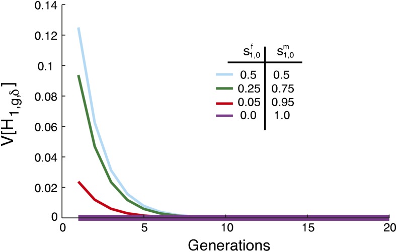
For the specific case of $s_{1,0}=\frac{1}{2}$, the total contribution for which the maximal variance occurs in Figure 3, we illustrate the variance at several locations in the allowed range for $s_{1,0}^{\text{f}}$ and $s_{1,0}^{\text{m}}$ (Figure 4). Four scenarios are plotted with the same total founding contribution from source population 1, $s_{1,0}=\frac{1}{2}$, but with different levels of sex bias. As the female and male contributions become increasingly different, the initial variance decreases. The largest variance for $s_{1,0}=\frac{1}{2}$ occurs at $s_{1,0}^{\text{f}}=s_{1,0}^{\text{m}}=s_{1,0}$, with no sex bias. The minimum occurs when males all come from one source population and females all from the other. In this extreme sex-biased case, the variance is zero constantly over time, as each individual has a male parent from one population, a female parent from the other, and an admixture fraction of $\frac{1}{2}$.

Figure 4.

The variance of the fraction of admixture, $\mathbb{V}$[H₁,g,δ], when contributions from the source populations occur only in the founding generation and the total contribution from source population 1 is held constant at $s_{1,0}=\frac{1}{2}$. The limit of the variance of the fraction of admixture over time is zero for any choice of $\left(s_{1,0}^{\text{f}},s_{1,0}^{\text{m}}\right)$. The magnitude of the variance, calculated from Equation 35, is inversely related to the level of sex bias. For all four scenarios, s₁ = s₂ = 0 and $s_{1,0}=s_{2,0}=\frac{1}{2}$.

Special Case: Constant Nonzero Contributions

Next, we consider the case in which an initial admixture event founds the hybrid population and is then followed by constant nonzero contributions from the source populations. After the founding, for each g ≥ 1, all admixture parameters are constant in time: $s_{\alpha ,g}^{\delta }=s_{\alpha }^{\delta }$ for each α ∈ {1, 2} and δ ∈ {f, m}, and $h_g^{\delta }=h^{\delta }$ for each δ. Thus, we have parameter values for the founding and constant continuing admixture parameters $s_1^{\text{f}}$, $s_1^{\text{m}}$, $s_2^{\text{f}}$, and $s_2^{\text{m}}$. Each parameter takes its value in [0, 1], as do s₁ and s₂. By contrast, h takes its value in (0, 1). The case of h = 1 is a single admixture event, analyzed above. The h = 0 case is trivial because the hybrid population is refounded at each generation, and the distribution of the admixture fraction thus depends only on the contribution in the previous generation. Therefore, we require s₁ + s₂ ≠ 0 and s₁ + s₂ ≠ 1. Individually, however, h^f and h^m can each vary in [0, 1], as long as they are not both zero or one.

The recursion for the expectation of the autosomal fraction of admixture, Equations 17 and 19, is equivalent to that derived by Verdu and Rosenberg (2011). Therefore, the closed form of the expectation is equivalent as well. From Verdu and Rosenberg (2011, Equation 30) we have

$$\mathbb{E}\left[H_{1,g,\delta }\right]=\{\begin{array}{ll}{s}_{1,0},\hfill & g=1\hfill \\ s_{1,0}{h}^{g-1}+s_1\frac{1-h^{g-1}}{1-h},\hfill & g\ge 2.\hfill \end{array}$$ (37)

We can use the same method as Verdu and Rosenberg (2011) to simplify the second moment. Under the special case of constant contributions across generations, for g = 1, Equation 29 gives

$$\mathbb{E}\left[H_{1,1,\delta }^2\right]=\frac{s_{1,0}^{\text{f}}\left(1+s_{1,0}^{\text{m}}\right)+s_{1,0}^{\text{m}}\left(1+s_{1,0}^{\text{f}}\right)}{4}.$$ (38)

For g ≥ 2, Equation 31 gives

$$\begin{array}{c}\mathbb{E}\left[H_{1,g,\delta }^2\right]=\frac{s_1^{\text{f}}\left(1+s_1^{\text{m}}\right)+s_1^{\text{m}}\left(1+s_1^{\text{f}}\right)}{4}+\frac{s_1^{\text{f}}{h}^{\text{m}}+h^{\text{f}}{s}_1^{\text{m}}}{2}\mathbb{E}\left[H_{1,g-1,\delta }\right]\\ +\frac{h^{\text{f}}{h}^{\text{m}}}{2}{\left(\mathbb{E}\left[H_{1,g-1,\delta }\right]\right)}^2+\frac{h^{\text{f}}+h^{\text{m}}}{4}\mathbb{E}\left[H_{1,g-1,\delta }^2\right].\end{array}$$ (39)

Because this equation is a nonhomogenous first-order recurrence with the form

$$\mathbb{E}\left[H_{1,g,\delta }^2\right]=\psi \left(g\right)+\lambda \mathbb{E}\left[H_{1,g-1,\delta }^2\right],$$ (40)

we can use Theorem 3.1.2 of Cull et al. (2005) to solve for a unique solution for $\mathbb{E}\left[H_{1,g,\delta }^2\right]$, as in Verdu and Rosenberg (2011). For the initial condition, we have

$${\alpha }_0=\mathbb{E}\left[H_{1,1,\delta }^2\right]=\frac{s_{1,0}^{\text{f}}\left(1+s_{1,0}^{\text{m}}\right)+s_{1,0}^{\text{m}}\left(1+s_{1,0}^{\mathrm{f}}\right)}{4}.$$ (41)

We define λ = (h^f + h^m)/4 = h/2, and for all g ≥ 2, we have

$$\psi \left(g\right)=\frac{s_1^{\text{f}}\left(1+s_1^{\text{m}}\right)+s_1^{\text{m}}\left(1+s_1^{\text{f}}\right)}{4}+\frac{s_1^{\text{f}}{h}^{\text{m}}+h^{\text{f}}{s}_1^{\text{m}}}{2}\mathbb{E}\left[H_{1,g-1,\delta }\right]+\frac{h^{\text{f}}{h}^{\text{m}}}{2}{\left(\mathbb{E}\left[H_{1,g-1,\delta }\right]\right)}^2.$$ (42)

Using the expected admixture fraction from Equation 37, we can simplify Equation 42. For all g ≥ 2,

$$\begin{array}{c}\psi \left(g\right)=\frac{s_1^{\text{f}}\left(1+s_1^{\text{m}}\right)+s_1^{\text{m}}\left(1+s_1^{\text{f}}\right)}{4}+\frac{s_1^{\text{f}}{h}^{\text{m}}+h^{\text{f}}{s}_1^{\text{m}}}{2}\left(s_{1,0}{h}^{g-2}+s_1\frac{1-h^{g-2}}{1-h}\right)\\ +\frac{h^{\text{f}}{h}^{\text{m}}}{2}{\left(s_{1,0}{h}^{g-2}+s_1\frac{1-h^{g-2}}{1-h}\right)}^2.\end{array}$$ (43)

Therefore, using Theorem 3.1.2 of Cull et al. (2005), we have a unique solution for $\mathbb{E}\left[H_{1,g,\delta }^2\right]$:

$$\mathbb{E}\left[H_{1,g,\delta }^2\right]=\{\begin{array}{ll}{\alpha }_0,\hfill & g=1\hfill \\ \hfill & \hfill \\ {\alpha }_0{\left(\frac{h}{2}\right)}^{g-1}\hfill & \hfill \\ +{\displaystyle \sum _{i=2}^g[\frac{s_1^{\text{f}}\left(1+s_1^{\text{m}}\right)+s_1^{\text{m}}\left(1+s_1^{\text{f}}\right)}{4}}\hfill & \hfill \\ +\frac{s_1^{\text{f}}{h}^{\text{m}}+h^{\text{f}}{s}_1^{\text{m}}}{2}\left(s_{1,0}{h}^{i-2}+s_1\frac{1-h^{i-2}}{1-h}\right)\hfill & \hfill \\ +\frac{h^{\text{f}}{h}^{\text{m}}}{2}{\left(s_{1,0}{h}^{i-2}+s_1\frac{1-h^{i-2}}{1-h}\right)}^2]{\left(\frac{h}{2}\right)}^{g-i},\hfill & g\ge 2.\hfill \end{array}$$ (44)

Equation 44 can be simplified by separating the sum and summing the resulting geometric series,

$$\mathbb{E}\left[H_{1,g,\delta }^2\right]=\{\begin{array}{ll}{\alpha }_0,\hfill & g=1,\hfill \\ A_1+A_2{h}^{g-1}+\left(A_3+A_4{\displaystyle \sum _{i=1}^{g-1}{\left(2h\right)}^i}\right){\left(\frac{h}{2}\right)}^{g-1},\hfill & g\ge 2,\hfill \end{array}$$ (45)

where α₀ is defined in Equation 41, and

$$A_1=\frac{s_1+s_1^{\text{f}}{s}_1^{\text{m}}}{\left(2-h\right)}+\frac{s_1\left(s_1^{\text{f}}{h}^{\text{m}}+h^{\text{f}}{s}_1^{\text{m}}\right)}{\left(1-h\right)\left(2-h\right)}+\frac{s_1^2{h}^{\text{f}}{h}^{\text{m}}}{{\left(1-h\right)}^2\left(2-h\right)},$$ (46)

$$A_2=\frac{1}{h}\left(s_1^{\text{f}}{h}^{\text{m}}+h^{\text{f}}{s}_1^{\text{m}}+\frac{2h^{\text{f}}{h}^{\text{m}}{s}_1}{1-h}\right)\left(s_{1,0}-\frac{s_1}{1-h}\right),$$ (47)

$$\begin{array}{c}{A}_3={\alpha }_0+\frac{h^{\text{f}}{h}^{\text{m}}{s}_1}{1-h}\left[\frac{2}{h}\left(\frac{s_1}{1-h}-s_{1,0}\right)-\frac{s_1}{\left(1-h\right)\left(2-h\right)}\right]\\ +\left(s_1^{\text{f}}{h}^{\text{m}}+h^{\text{f}}{s}_1^{\text{m}}\right)\left[\frac{s_{1}h}{1-h}-s_{1,0}h-\frac{s_1}{\left(1-h\right)\left(2-h\right)}\right]-\frac{s_1+s_1^{\text{f}}{s}_1^{\text{m}}}{2-h},\end{array}$$ (48)

$$A_4=\frac{h^{\text{f}}{h}^{\text{m}}}{2h^2}\left[s_{1,0}^2+\frac{s_1}{1-h}\left(\frac{s_1}{1-h}-2s_{1,0}\right)\right].$$ (49)

When $s_1^{\text{f}}=s_1^{\text{m}}$ and $s_2^{\text{f}}=s_2^{\text{m}}$, A₁, A₂, A₃, and A₄ are equal to the corresponding quantities in Verdu and Rosenberg (2011, Equations 39–42). Therefore, without sex bias, the closed form of the second moment of the admixture fraction, Equation 45, is equal to Equation 38 in Verdu and Rosenberg (2011).

Using the relation $\mathbb{V}\left[H_{1,g,\delta }\right]=\mathbb{E}\left[H_{1,g,\delta }^2\right]-{\left(\mathbb{E}\left[H_{1,g,\delta }\right]\right)}^2$ and Equations 37 and 45, for the variance of the autosomal fraction of admixture, we have

$$\mathbb{V}\left[H_{1,g,\delta }\right]=\{\begin{array}{ll}\frac{s_{1,0}^{\text{f}}\left(1-s_{1,0}^{\text{f}}\right)+s_{1,0}^{\text{m}}\left(1-s_{1,0}^{\text{m}}\right)}{4},\hfill & g=1,\hfill \\ A_1+A_2{h}^{g-1}+\left[A_3+A_4{\displaystyle \sum _{i=1}^{g-1}{\left(2h\right)}^i}\right]{\left(\frac{h}{2}\right)}^{g-1}-{\left(s_{1,0}{h}^{g-1}+s_1\frac{1-h^{g-1}}{1-h}\right)}^2,\hfill & g\ge 2.\hfill \end{array}$$ (50)

For $h\ne \frac{1}{2}$, we have

$$\mathbb{V}\left[H_{1,g,\delta }\right]=\{\begin{array}{ll}\frac{s_{1,0}^{\text{f}}\left(1-s_{1,0}^{\text{f}}\right)+s_{1,0}^{\text{m}}\left(1-s_{1,0}^{\text{m}}\right)}{4},\hfill & g=1,\hfill \\ A_1+A_2{h}^{g-1}+\left[A_3+A_4\left(\frac{2h-{\left(2h\right)}^g}{1-2h}\right)\right]{\left(\frac{h}{2}\right)}^{g-1}-{\left(s_{1,0}{h}^{g-1}+s_1\frac{1-h^{g-1}}{1-h}\right)}^2,\hfill & g\ge 2.\hfill \end{array}$$ (51)

For $h=\frac{1}{2}$, Equation 50 gives

$$\mathbb{V}\left[H_{1,g,\delta }\right]=\{\begin{array}{ll}\frac{s_{1,0}^{\text{f}}\left(1-s_{1,0}^{\text{f}}\right)+s_{1,0}^{\text{m}}\left(1-s_{1,0}^{\text{m}}\right)}{4},\hfill & g=1,\hfill \\ A_1+A_2{\left(\frac{1}{2}\right)}^{g-1}+A_3{\left(\frac{1}{4}\right)}^{g-1}+A_4\left(g-1\right){\left(\frac{1}{4}\right)}^{g-1}-{\left[2s_1+\left(s_{1,0}-2s_1\right){\left(\frac{1}{2}\right)}^{g-1}\right]}^2,\hfill & g\ge 2.\hfill \end{array}$$ (52)

Equations 50–52 simplify to Equations 43–45 of Verdu and Rosenberg (2011) when $s_1^{\text{f}}=s_1^{\text{m}}$ and $s_2^{\text{f}}=s_2^{\text{m}}$.

Limiting variance of admixture over time

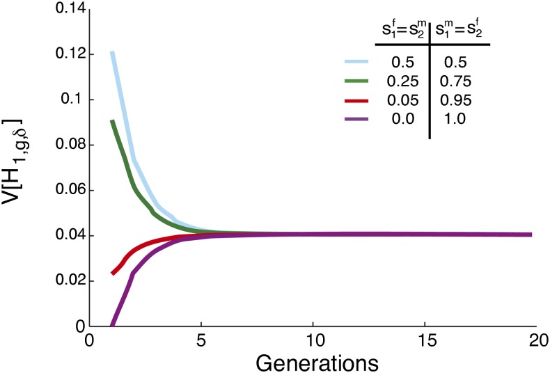
Figure 5 illustrates the variance of the autosomal fraction of admixture as a function of g when the contributions from the source populations are constant over time, computed using Equation 50. The figure shows that if the continuing contributions are held constant, then the long-term limiting variance does not depend on the founding parameters. Unlike in the hybrid isolation case, with constant, nonzero contributions from the source populations over time, h ≠ 0 and h ≠ 1, a nonzero limit is reached. Applying Equation 50,

$$\underset{g\to \mathrm{\infty }}{\lim }\mathbb{V}\left[H_{1,g,\delta }\right]=A_1-{\left(\frac{s_1}{1-h}\right)}^2,$$ (53)

which does not depend on the founding parameters. The limit matches that of Verdu and Rosenberg (2011, Equation 46) in the absence of sex bias ($s_1^{\text{f}}=s_1^{\text{m}}=s_1$, h^f = h^m = h, and $s_2^{\text{f}}=s_2^{\text{m}}=s_2$).

Figure 5.

The variance of the fraction of admixture over time for constant, nonzero contributions from the source populations, with different levels of sex bias in the founding of the hybrid population, and constant, equal, and nonzero subsequent contributions from the source populations and sex for g ≥ 1. In all cases, $s_1^{\text{f}}=s_1^{\text{m}}=s_2^{\text{f}}=s_2^{\text{m}}=0.2$. The variance, calculated with Equation 50, reaches a nonzero limit ${\lim }_{g\to \mathrm{\infty }}\mathbb{V}\left[H_{1,g,\delta }\right]=1/24$.

The maxima and minima of the limiting variance

Using Equations 1, 2, 4, and 46, the limit in Equation 53 can be equivalently written in terms of the two female sex-specific contributions, $s_1^{\text{f}}$ and $s_2^{\text{f}}$, and the total contributions from the two source populations, s₁ and s₂. Considering admixture scenarios with constant s₁, s₂, with s₁ + s₂ ∈ (0, 1], but allowing $s_1^{\text{f}}$ and $s_2^{\text{f}}$ to range over the closed unit interval, the limiting variance depends on two independent parameters, $s_1^{\text{f}},s_2^{\text{f}}\in \left[0,1\right]$, subject to the constraint in Equation 1:

$$\underset{g\to \mathrm{\infty }}{\lim }\mathbb{V}\left[H_{1,g,\delta }\right]=\frac{-{\left(s_1^{\text{f}}{s}_2-s_2^{\text{f}}{s}_1\right)}^2+s_1{s}_2\left(s_1+s_2\right)}{{\left(s_1+s_2\right)}^2\left(1+s_1+s_2\right)}.$$ (54)

Treating s₁ and s₂ as constants in [0,1], the critical points of Equation 54 are the same as those of

$$f\left(s_1^{\text{f}},s_2^{\text{f}}\right)=-{\left(s_1^{\text{f}}{s}_2-s_2^{\text{f}}{s}_1\right)}^2.$$ (55)

First we consider the maximum. Because $f\left(s_1^{\text{f}},s_2^{\text{f}}\right)$ is always negative or zero, the maximal variance given s₁ and s₂ occurs when $f\left(s_1^{\text{f}},s_2^{\text{f}}\right)=0$, which occurs on the line $s_1^{\text{f}}{s}_2=s_2^{\text{f}}{s}_1$. Equivalently, recalling Equation 1,

$$\frac{s_1^{\text{f}}}{s_2^{\text{f}}}=\frac{s_1^{\text{m}}}{s_2^{\text{m}}}=\frac{s_1}{s_2}.$$ (56)

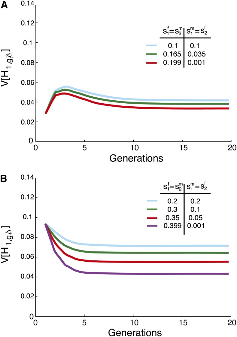
Equation 56 has many solutions for $\left(s_1^{\text{f}},s_1^{\text{m}},s_2^{\text{f}},s_2^{\text{m}}\right)$ given s₁ and s₂. One solution is $\left(s_1^{\text{f}},s_2^{\text{f}}\right)=\left(s_1,s_2\right)$, which by Equation 1 is equivalent to $\left(s_1^{\text{f}},s_2^{\text{f}}\right)=\left(s_1^{\text{m}},s_2^{\text{m}}\right)$. Therefore, the limiting variance of the admixture fraction is maximized when there is no sex bias. Figure 6 plots two examples of the variance for constant s₁ and s₂, but increasingly different sex-specific contributions from the source populations. In Figure 6, A and B, the admixture history with no sex bias produces the greatest limit.

Figure 6.

The variance of the fraction of admixture over time for constant, nonzero contributions from the source populations, with different levels of sex bias, but the same total contribution from the two source populations. (A) $s_{1,0}^{\text{f}}=s_{1,0}^{\text{m}}=0.9$ and s₁ = s₂ = 0.1. (B) $s_{1,0}^{\text{f}}=s_{1,0}^{\text{m}}=0.75$ and s₁ = s₂ = 0.2. The variance reaches a nonzero limit when $s_1^{\text{f}}$, $s_1^{\text{m}}$, $s_2^{\text{f}}$, and $s_2^{\text{m}}$ are nonzero and constant over time. The variance is calculated using Equation 50.

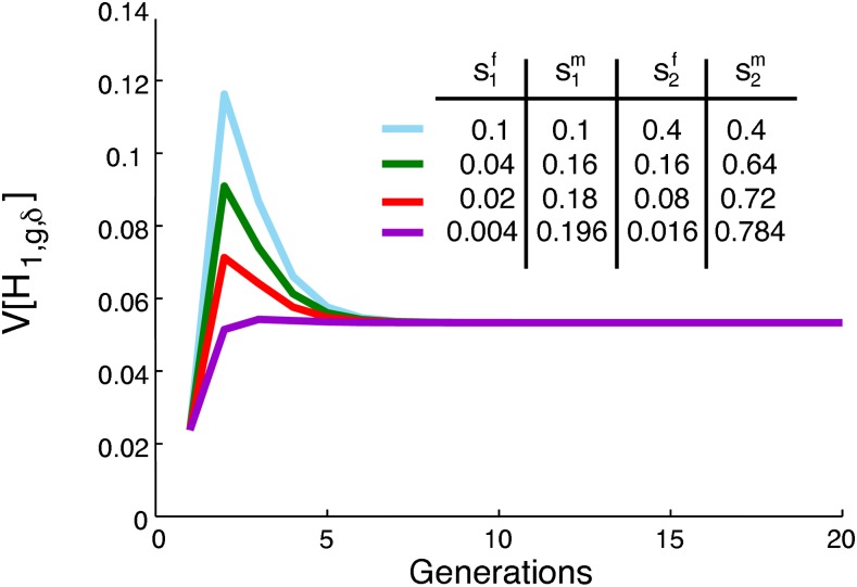
For fixed s₁ and s₂, however, the case without sex bias is not the only maximum of the limiting variance. Figure 7 plots the variance over time for four different admixture histories, each with the same total contributions s₁ and s₂, but quite different sex-specific contributions $\left(s_1^{\text{f}},s_1^{\text{m}},s_2^{\text{f}},s_2^{\text{m}}\right)$. Each of the four scenarios plotted reaches the same limit because each provides a solution to Equation 56. Because $f\left(s_1^{\text{f}},s_2^{\text{f}}\right)=0$, Equation 54 depends only on the total contributions s₁ and s₂. For constant s₁ and s₂, any admixture history whose contributions solve $f\left(s_1^{\text{f}},s_2^{\text{f}}\right)=0$ has limiting variance

$$\underset{g\to \mathrm{\infty }}{\lim }\mathbb{V}\left[H_{1,g,\delta }\right]=\frac{s_1{s}_2}{\left(s_1+s_2\right)\left(1+s_1+s_2\right)}.$$ (57)

This maximal limiting variance depends on the total contributions from the source populations, but not on the sex-specific contributions; it is equivalent to Equation 47 of Verdu and Rosenberg (2011).

Figure 7.

The variance of the fraction of admixture over time for constant, nonzero contributions from the source populations, but multiple different ratios of female to male contributions. When the sex-specific parameters satisfy the equation $s_1^{\text{f}}{s}_2^{\text{m}}=s_1^{\text{m}}{s}_2^{\text{f}}$, different demographic scenarios have the same limiting variance of the admixture fraction. In all cases, ${\text{lim}}_{g\to \mathrm{\infty }}\mathbb{V}\left[H_{1,g,\delta }\right]=\frac{4}{75}$. The variance is calculated using Equation 33. For all scenarios, $s_{1,0}^{\text{f}}=s_{1,0}^{\text{m}}=0.95$.

Thus far, we have considered the maximal limiting variance as a function of the sex-specific parameters given constant total contributions s₁ and s₂. We can also identify the values of s₁ and s₂ that maximize the limiting variance, considering all s₁, s₂ ∈ [0, 1]. For each choice of s₁ and s₂, the maximal variance over values of $s_1^f$ and $s_2^f$ is given by Equation 57. We can therefore find the s₁ and s₂ that maximize Equation 57. As shown by Verdu and Rosenberg (2011), given s₁ + s₂, the maximal limiting variance occurs when s₁ = s₂. Over the range of possible choices for s₁ + s₂ ∈ (0, 1), the maximum occurs when $s_1=s_2=\frac{1}{2}$. Unlike in Verdu and Rosenberg (2011), however, this maximum requires the sex-specific contributions to solve $f\left(s_1^{\text{f}},s_2^{\text{f}}\right)=0$.

Interestingly, one of the minima of the limiting variance occurs when $s_1=s_2=\frac{1}{2}$, but with $f\left(s_1^{\text{f}},s_2^{\text{f}}\right)\ne 0$. Specifically, when $s_1=s_2=\frac{1}{2}$, but all males come from one source population and all females from the other, $\left(s_1^{\text{f}},s_1^{\text{m}},s_2^{\text{f}},s_2^{\text{m}}\right)=\left(1,0,0,1\right)$ or (0, 1, 1, 0), the limiting variance in Equation 54 is zero. In this case, $L=S_1{S}_2$ or $L=S_2{S}_1$ for every individual in the hybrid population. By Equation 8, the hybrid population is founded anew at each generation, each individual having admixture fraction $H_{1,g,\delta }=\frac{1}{2}$.

More generally, given $s_1$ and $s_2$, the minimum occurs when $\left(s_1^{\text{f}},s_2^{\text{f}}\right)=\left(2s_1,0\right)$ or $\left(s_1^{\text{f}},s_2^{\text{f}}\right)=\left(0,2s_2\right)$. Given $s_1$ and $s_2$, the limiting variance is minimized with respect to $s_1^{\text{f}}$ and $s_2^{\text{f}}$ when $f\left(s_1^{\text{f}},s_2^{\text{f}}\right)$ is smallest (Equation 54). Because f is the negative of the square of a difference of products, it is smallest when one term is zero and the other is at its maximum, as at $\left(s_1^{\text{f}},s_2^{\text{f}}\right)=\left(2s_1,0\right)$ or $\left(s_1^{\text{f}},s_2^{\text{f}}\right)=\left(0,2s_2\right)$. These points represent the maximal sex bias for fixed (s₁, s₂).

If we allow s₁ and s₂ to vary, because a variance is bounded below by zero, any set of parameters that produces zero variance is a minimum. In Equation 54, if either s₁ = 0 or s₂ = 0, then the limiting variance of the admixture fraction is zero. When only one population contributes after the founding, in the limit, all ancestry in the hybrid population traces to that population.

Properties of the limiting variance

The limiting variance of the fraction of admixture over time in Equation 53 is a function of the sex-specific contributions from the hybrid population, h^f and h^m, and source population 1, $s_1^{\text{f}}$ and $s_1^{\text{m}}$. Recalling Equation 4, the limiting variance is equivalently written as a function of the sex-specific contributions from source population 2, $s_2^{\text{f}}$ and $s_2^{\text{m}}$, and either source population 1 (Equation 54), or the hybrid population. It can be viewed as a function of all six sex-specific parameters $\left(s_1^{\text{f}},s_1^{\text{m}},s_2^{\text{f}},s_2^{\text{m}},h^{\text{f}},h^{\text{m}}\right)$, four of which can be selected while assigning the other two by the constraint from Equation 4.

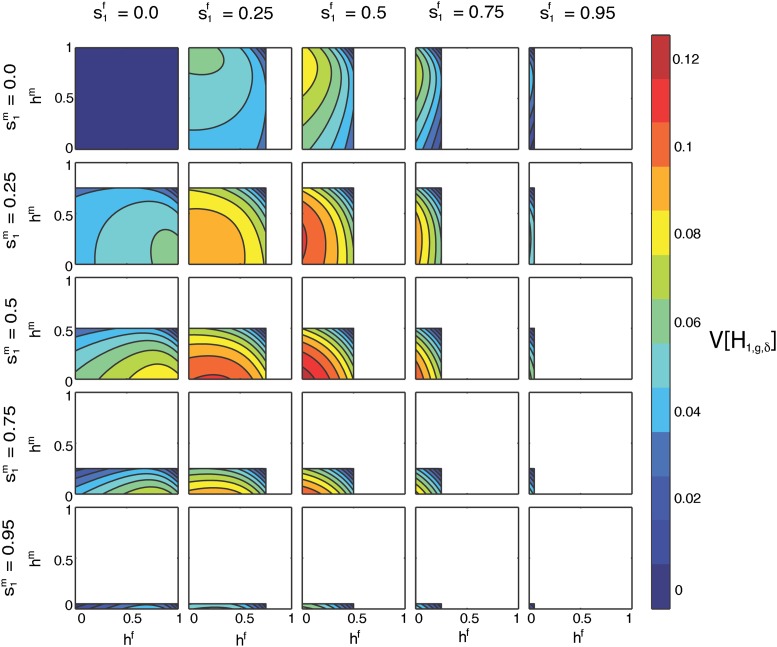
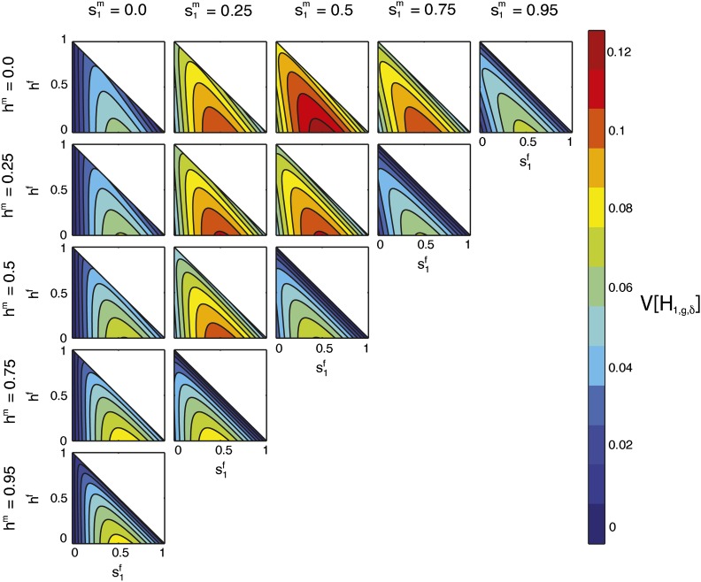
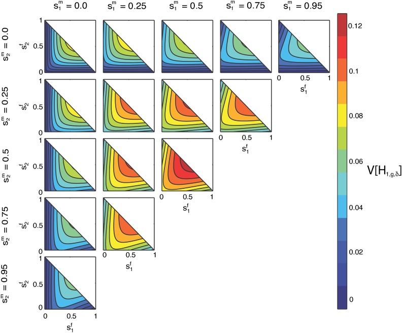
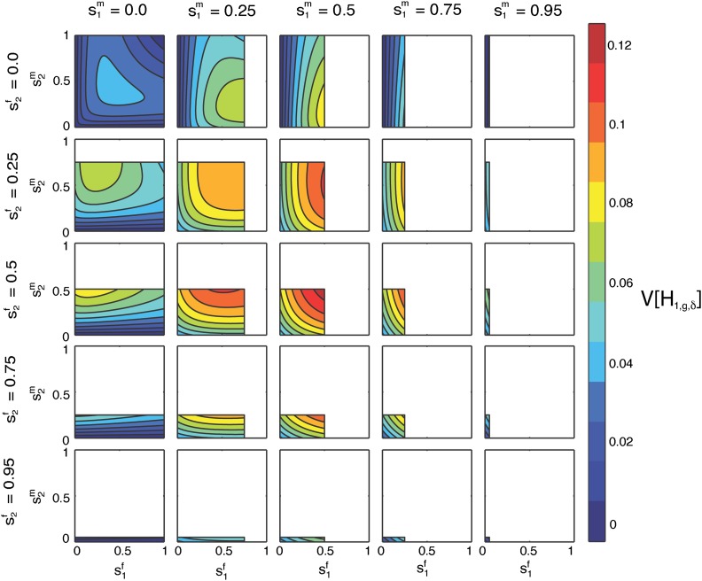
We can therefore analyze the behavior of the limiting variance as a function of two of the sex-specific parameters by specifying two other parameters and allowing the final two parameters, one female and one male, to vary according to Equation 4. Of the four parameters we consider, using the constraint from Equation 4 separately in males and females, two must be male and two must be female. Because the variance is invariant with respect to exchanging the source populations or the sexes, the six-dimensional parameter space has a number of symmetries. Figure 8, Figure 9, Figure 10, Figure 11, and Figure 12 examine the five possible, nonredundant ways of choosing two populations and the corresponding male and female parameters from those populations and holding two corresponding parameters fixed (either from the same sex in the two populations, or for males and females from one population) while allowing the other two to vary. Figure 13 then highlights an informative case that considers the limiting variance in terms of a male and a female parameter from different populations.

Figure 8.

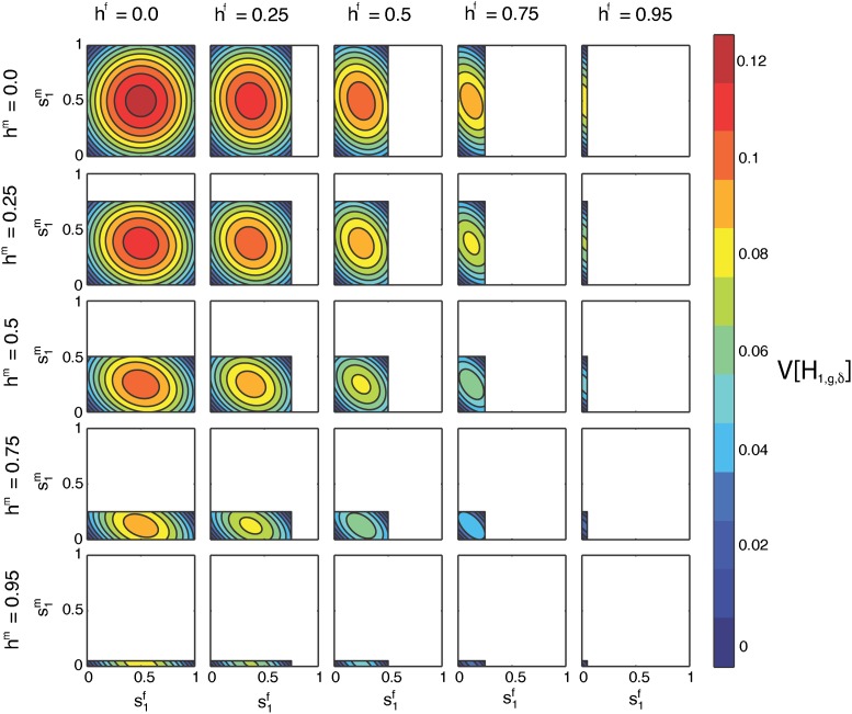
Contour plots of the limit of the variance of the fraction of admixture over time as a function of $s_1^{\text{f}}$ on the x-axis and $s_1^{\text{m}}$ on the y-axis for specified values of h^f by column and h^m by row. The domains of $s_1^{\text{f}}$ and $s_1^{\text{m}}$ are [0, 1 − h^f] and [0, 1 − h^m], respectively.

Figure 9.

Contour plots of the limit of the variance of the fraction of admixture over time as a function of $s_1^{\text{f}}$ on the x-axis and $s_1^{\text{m}}$ on the y-axis for specified values of $s_2^{\text{f}}$ by column and $s_2^{\text{m}}$ by row. The domains of $s_1^{\text{f}}$ and $s_1^{\text{m}}$ are $\left[0,1-s_2^{\text{f}}\right]$ and $\left[0,1-s_2^{\text{m}}\right]$, respectively.

Figure 10.

Contour plots of the limit of the variance of the fraction of admixture over time as a function of h^f on the x-axis and h^m on the y-axis for specified values of $s_1^{\text{f}}$ by column and $s_1^{\text{m}}$ by row. The domains of h^f and h^m are $\left[0,1-s_1^{\text{f}}\right]$ and $\left[0,1-s_1^{\text{m}}\right]$, respectively.

Figure 11.

Contour plots of the limit of the variance of the fraction of admixture over time as a function of $s_1^{\text{f}}$ on the x-axis and h^f on the y-axis for specified values of $s_1^{\text{m}}$ by column and h^m by row. The domains of $s_1^{\text{f}}$ and h^f are bounded below by 0 and above by the line $s_1^{\text{f}}+h^{\text{f}}=1$.

Figure 12.

Contour plots of the limit of the variance of the fraction of admixture over time as a function of $s_1^{\text{f}}$ on the x-axis and $s_2^{\text{f}}$ on the y-axis for specified values of $s_1^{\text{m}}$ by column and $s_2^{\text{m}}$ by row. The domains of $s_1^{\text{f}}$ and $s_2^{\text{f}}$ are bounded below by 0 and above by the line $s_1^{\text{f}}+s_2^{\text{f}}=1.$

Figure 13.

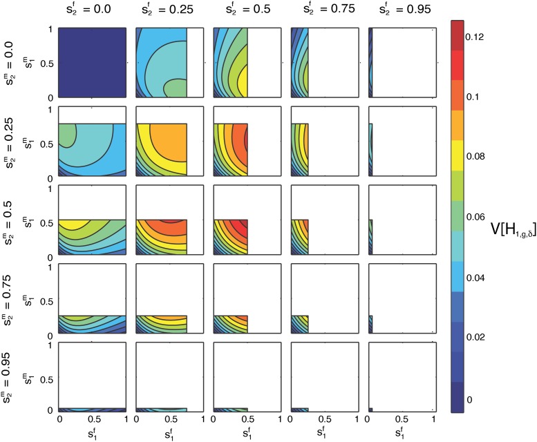
Contour plots of the limit of the variance of the fraction of admixture over time as a function of $s_1^{\text{f}}$ on the x-axis and $s_2^{\text{m}}$ on the y-axis for specified values of $s_2^{\text{f}}$ by column and $s_1^{\text{m}}$ by row. The domains of $s_1^{\text{f}}$ and $s_2^{\text{m}}$ are $\left[0,1-s_2^{\text{f}}\right]$ and $\left[0,1-s_1^{\text{m}}\right]$, respectively.

Each figure shows multiple contour plots of the limiting variance as a function of two sex-specific parameters, for fixed values of two other parameters. Three cases plot the limiting variance as a function of the female and male parameters from a given population, with the female and male contributions of another population specified. In two other cases, parameters for a single sex from two populations are plotted, specifying the contributions from the other sex for those populations.

By considering these parameter combinations, we can examine the dependence of the variance on sex-specific parameters and parameter interactions, as well as potential bounds on both the parameters and the variance. We highlight a number of symmetries in the limiting variance. The plots also illustrate the maxima and minima found in the previous section.

Properties of the limiting variance in terms of ${\mathit{s}}_1^{\text{f}}$ and ${\mathit{s}}_1^{\text{m}}$:

In Figure 8, we consider the variance of the fraction of admixture as a function of $s_1^{\text{f}}$, the female contribution from S₁, on the x-axis, and $s_1^{\text{m}}$, the male contribution from S₁, on the y-axis, computed using Equation 53. We plot the variance for fixed h^f, the female contribution from H, and h^m, the male contribution from H. The domain for $s_1^{\text{f}}$ and $s_1^{\text{m}}$ is constrained by Equation 4, with $s_1^{\text{f}}$ taking values in [0, 1 − h^f], and $s_1^{\text{m}}$ taking values in [0, 1 − h^m].

Figure 8, top left, shows the variance as a function of $s_1^{\text{f}}$ and $s_1^{\text{m}}$, with h^f = h^m = h = 0. Here, the hybrid population is founded anew by the source populations each generation, and $s_1^{\text{f}}$ and $s_1^{\text{m}}$ both take values from the full domain [0, 1]. For h^f = h^m = h = 0, the maximal limiting variance is ${\lim }_{g\to \mathrm{\infty }}\mathbb{V}\left[H_{1,g,\delta }\right]=\frac{1}{8}$, occurring when $s_1^{\text{f}}=s_1^{\text{m}}=s_1=0.5$. At this maximum, given Equation 4 and h^f = h^m = 0, we have $s_2^{\text{f}}=s_2^{\text{m}}=s_2=0.5$. As in Equation 54, the maximum occurs when female and male contributions from the source populations are equal and the total contributions from the source populations are equal.

The minima of ${\lim }_{g\to \mathrm{\infty }}\mathbb{V}\left[H_{1,g,\delta }\right]=0$ occur at the four corners of the plot. At the origin, when $s_1^{\text{f}}=s_1^{\text{m}}=s_1=0$, the limiting variance is zero because only S₂ contributes to the hybrid population. Individuals in the hybrid population all have parents L = S₂S₂ and admixture fraction zero (Equation 8). By exchanging S₁ for S₂, the case of $s_1^{\text{f}}=s_1^{\text{m}}=s_1=1$ is similar. Additional minima occur at $\left(s_1^{\text{f}},s_1^{\text{m}}\right)=\left(1,0\right)$ or (0, 1), where all males come from one source population and all females from the other, and all individuals at the next generation of the hybrid population have admixture fraction $\frac{1}{2}$ (Equation 8).

For h^f = h^m = h = 0, the limiting variance is symmetrical over the line $s_1^{\text{m}}=s_1^{\text{f}}$, as a result of the symmetry between males and female in the variance (Equation 33). Because the hybrid population provides no contribution and the variance of the fraction of admixture is symmetric with respect to source population, the variance is also symmetric over the lines $s_1^{\text{f}}=0.5$ and $s_1^{\text{m}}=0.5$.

The columns of Figure 8 consider increasing, fixed values for h^f, and the rows consider increasing, fixed values for h^m, both from {0, 0.25, 0.5, 0.75, 0.95}. All the cells maintain the general shape of the limiting variance as a function of $s_1^{\text{f}}$ and $s_1^{\text{m}}$ seen for h^f = h^m = 0. However, as the domain for $s_1^{\text{f}}$ and $s_1^{\text{m}}$ shrinks with increasing h^f and h^m, the location of the maximal variance changes across cells. In all cases, the maximum of the limiting variance occurs when $s_1^{\text{f}}$ and $s_1^{\text{m}}$ each lie at the midpoints of their respective domains, $s_1^{\text{f}}=\left(1-h^{\text{f}}\right)/2$ and $s_1^{\text{m}}=\left(1-h^{\text{m}}\right)/2.$ The magnitude of the limiting variance at each maximum decreases as its location moves away from $s_1^{\text{f}}=s_1^{\text{m}}=0.5$.

In all the cells, the minimum ${\lim }_{g\to \mathrm{\infty }}\mathbb{V}\left[H_{1,g,\delta }\right]=0$ occurs when $s_1^{\text{f}}$ and $s_1^{\text{m}}$ are either both zero or they lie at the maxima of their respective domains. In these cases, only one source population contributes to the hybrid population, and all individuals in the hybrid population have an admixture fraction from S₁ of either 0, when $s_1^{\text{f}}=s_1^{\text{m}}=0$, or 1, when $s_1^{\text{f}}=1-h^{\text{f}}$ and $s_1^{\text{m}}=1-h^{\text{m}}$. The limiting variance is no longer zero at the two corners of each plot where only one of $\left\{s_1^{\text{f}},s_1^{\text{m}}\right\}$ is at the maximum of its domain; these corners, however, are minima of the variance given the values of s₁ and s₂. In these cases, males all come from one source population and females from the other, producing a minimum of Equation 54 for fixed s₁ and s₂.

As in the case of h^f = h^m = 0, each cell is symmetrical in reflecting over both the midpoint of the x-axis, $s_1^{\text{f}}=\left(1-h^{\text{f}}\right)/2$, and that of the y-axis, $s_1^{\text{m}}=\left(1-h^{\text{m}}\right)/2$. The limiting variance is symmetrical with respect to source population (Equation 54), and this pair of reflections corresponds to an exchange of source populations. For h^f = h^m = 0, the line $s_1^{\text{f}}=s_1^{\text{m}}$ generates circular contours, but as the contributions from the hybrid population increase, the contours become elliptical.

In Figure 8, cells on the diagonal have equal contributions from males and females in the hybrid population, h^f = h^m = h. For h^f ≠ h^m, cells above the diagonal are equivalent to those below the diagonal with an exchange of female for male contributions, for both s₁ and h. For example, the cell with h^f = 0.25 and h^m = 0.5 is equivalent to the cell with h^f = 0.5 and h^m = 0.25 if the axes are also switched so that $s_1^{\text{m}}$ appears along the x-axis and $s_1^{\text{f}}$ is on the y-axis.

Figure 9 plots the limiting variance as a function of $s_1^{\text{f}}$ on the x-axis and $s_1^{\text{m}}$ on the y-axis, but we now fix values of $s_2^{\text{f}}$ by column and $s_2^{\text{m}}$ by row using Equations 54 and 1. The maxima and minima occur at the same parameter values found in Figure 8, but they appear in different locations on the plots. For example, in Figure 9, the global maximum across cells occurs in the plot with $s_2^{\text{f}}=s_2^{\text{m}}=0.5$ specified, and $s_1^{\text{f}}=s_2^{\text{m}}=0.5$. By Equation 4, this location has h^f = h^m = 0, the cell with the maximal variance in Figure 8. In Figure 9, top left, the variance is zero for all $s_1^{\text{f}}$ and $s_1^{\text{m}}$, because s₂ = 0 (Equation 54).

Whereas all cells in Figure 8 are symmetric in reflecting over the midpoints of both domains, in Figure 9, only the cells with $s_2^{\text{f}}=s_2^{\text{m}}$ are symmetric over the line $s_1^{\text{m}}=s_1^{\text{f}}.$ However, the symmetry corresponding to transposing males and females is visible in that a cell above the diagonal and its corresponding cell below the diagonal are equivalent if the axes for $s_1^{\text{f}}$ and $s_1^{\text{m}}$ are switched.

Properties of the limiting variance in terms of h^f and h^m:

Similarly to Figure 8, Figure 10 considers the limiting variance of the admixture fraction over time as a function of the four variables $s_1^{\text{f}}$, $s_1^{\text{m}}$, h^f, and h^m using Equation 53. In Figure 10, each cell shows h^f on the x-axis and h^m on the y-axis, for $s_1^{\text{f}}$ and $s_1^{\text{m}}$ specified, with the domains of h^f and h^m constrained by Equation 4. The cells on the diagonal have $s_1^f=s_1^m$, and there is a symmetry over this line of cells in that if values of $s_1^{\text{f}}$ and $s_1^{\text{m}}$ are switched, then the cells will be equivalent with a transposition of the axes.

In Figure 10, top left, $s_1^{\text{f}}=s_1^{\text{m}}=s_1=0$, and the limiting variance is a constant zero. In Figure 10, the maximal variance occurs at the origin (h^f = h^m = h = 0) of the cell with $s_1^{\text{f}}=s_1^{\text{m}}=s_1=0.5$. As in Figure 8, at the maximum, by Equation 4, $s_2^{\text{f}}=s_2^{\text{m}}=s_2=0.5$. In this case, females and males contribute equally. Both source populations contribute maximally to pull the distribution of the fraction of admixture toward the extremes of zero and one.

Because the limiting variance is symmetrical with respect to source population, and recalling Equation 4, each cell in Figure 10 is equivalent to a corresponding cell in Figure 9 reflected along both the x-axis and y-axis. For example, the cell in Figure 10 with $s_1^{\text{f}}=0.5$ and $s_1^{\text{m}}=0.25$ is equivalent to the Figure 9 cell with $s_2^{\text{f}}=0.5$ and $s_2^{\text{m}}=0.25$ if reflected on both the x- and y-axes.

Figure 8, Figure 9, and Figure 10 illustrate that the global maximum of the limiting variance occurs when the two source populations contribute equally, the contributions from the two sexes are equal, and the hybrid population does not contribute to the next generation. As the parameters move from the location of the maximal limiting variance to the minimum, the variance monotonically decreases.

Properties of the limiting variance in terms of ${\mathit{s}}_1^{\text{f}}$, h^f, and ${\mathit{s}}_2^{\text{f}}$:

Next we plot on the x- and y-axes two parameters of the same sex from different populations. Because the variance is invariant with respect to transposition of females and males, we consider only females without loss of generality. Figure 11 plots the limiting variance as a function of $s_1^{\text{f}}$ on the x-axis and h^f on the y-axis, for fixed values of $s_1^{\text{m}}$ and h^m. Figure 12 plots the limiting variance as a function of $s_1^{\text{f}}$ and $s_2^{\text{f}}$, for fixed $s_1^{\text{m}}$ and $s_2^{\text{m}}$. For Figure 11 and Figure 12, the domains of $s_1^{\text{f}},s_2^{\text{f}},$ and h^f are constrained by Equation 4.

For Figure 11, the maximal limiting variance occurs in the cell with $s_1^{\text{m}}=0.5$ and h^m = 0, at $\left(s_1^{\text{f}},h^{\text{f}}\right)=\left(0.5,0\right)$. By Equation 4, this location is the same parameter set for the maximum in Figures 8, Figure 9, and Figure 10. The maximum in each cell occurs when $\left(s_1^{\text{f}},h^{\text{f}}\right)=\left(0.5,0\right)$, but the magnitude of the variance decreases with increased distance from the cell with fixed $s_1^{\text{m}}=0.5$ and h^m = 0. Similarly, within each cell, the limiting variance decreases with distance from $\left(s_1^{\text{f}},h^{\text{f}}\right)=\left(0.5,0\right)$.

In the first column of Figure 11, where $s_1^{\text{m}}=0$, the line $s_1^{\text{f}}=0$ produces zero variance because the hybrid population is homogenous, with only one source population contributing. Similarly, in cells with $s_1^{\text{m}}+h^{\text{m}}=1$, as $s_2^{\text{f}}=s_2^{\text{m}}=0$ by Equation 4, the line $s_1^{\text{f}}+h^{\text{f}}=1$ has minimal variance.

In Figure 12, because of the symmetry in sex in Equation 54, the cells above and below those where $s_1^{\text{m}}=s_2^{\text{m}}$ are equivalent with a transposition of axes. As in Figure 8, Figure 9, Figure 10, and Figure 11, the maximal variance occurs in the cell with $s_1^{\text{m}}=s_2^{\text{m}}=0.5$ at $s_1^{\text{f}}=s_2^{\text{f}}=\mathrm{0.5.}$ Also, similar to Figure 11, in the first column, when $s_1^{\text{m}}=0,$ the line $s_1^{\text{f}}=0$ is a minimum; in the first row, when $s_2^{\text{m}}=0,$ the line $s_2^{\text{f}}=0$ is a minimum.

Analogous to the similarity between Figure 9 and Figure 10, by Equation 4, each cell in Figure 12 is a transformation of a cell in Figure 11. For example, for the cell with $s_1^{\text{m}}=0.25$ and h^m = 0.5 specified in Figure 11, because the male contributions sum to one, this cell also specifies $s_2^{\text{m}}=0.25$. Therefore, we can compare this cell to the cell with $s_1^{\text{m}}=s_2^{\text{m}}=0.25$ in Figure 12. Both show $s_1^{\text{f}}$ on the x-axis, and using Equation 4, we can rewrite the y-axis in Figure 12 as $s_2^{\text{f}}=1-h^{\text{f}}$.

Properties of the limiting variance in terms of noncorresponding parameters:

Finally, we consider a case in which males from one population in (S₁, S₂, H) are compared to females from a different population. Although multiple parameter configurations are possible, we plot one that is particularly informative, providing a perspective on Equation 54 beyond the observations visible in Figure 8, Figure 9, Figure 10, Figure 11, and Figure 12. Figure 13 plots the limit of the variance of the admixture fraction as a function of $s_1^{\text{f}}$ on the x-axis and $s_2^{\text{m}}$ on the y-axis, for fixed $s_2^{\text{f}}$ and $s_1^{\text{m}}$. We rewrite Equation 54 as a function of $s_1^{\text{f}},s_1^{\text{m}},s_2^{\text{f}}$, and $s_2^{\text{m}}$ using Equation 1:

$$\underset{g\to \mathrm{\infty }}{\lim }\mathbb{V}\left[H_{1,g,\delta }\right]=\frac{-2{\left(s_1^{\text{f}}{s}_2^{\text{m}}-s_2^{\text{f}}{s}_1^{\text{m}}\right)}^2+\left(s_1^{\text{f}}+s_1^{\text{m}}\right)\left(s_2^{\text{f}}+s_2^{\text{m}}\right)\left(s_1^{\text{f}}+s_1^{\text{m}}+s_2^{\text{f}}+s_2^{\text{m}}\right)}{{\left(s_1^{\text{f}}+s_1^{\text{m}}+s_2^{\text{f}}+s_2^{\text{m}}\right)}^2\left(2+s_1^{\text{f}}+s_1^{\text{m}}+s_2^{\text{f}}+s_2^{\text{m}}\right)}.$$ (58)

The limit depends on products of sex-specific parameters, including $s_1^{\text{f}}{s}_2^{\text{m}}$, as can be seen in the shape of the contours in Figure 13, but not in the analogous plots in Figure 9.

Discussion

Our model demonstrates the potential informativeness of autosomal DNA in the study of sex-biased admixture histories. Under a framework in which admixture occurs over time, potentially with different male and female contributions from the source populations, we have derived recursive expressions for the expectation, variance, and higher moments of the fraction of autosomal admixture. For the special case of constant admixture over time, we have analyzed the behavior of the variance of the admixture fraction. Although the expectation of the autosomal admixture fraction depends only on the total contributions from the source populations, we found that the variance of the autosomal admixture can contain a signature of sex-specific contributions. In particular, for constant admixture over time, the variance of the autosomal admixture fraction decreases as the male and female contributions become increasingly unequal.

That autosomal DNA possesses a signature of sex-biased admixture might at first appear counterintuitive, as unlike the sex chromosomes, autosomes are carried equally in both sexes. The phenomenon can, however, be understood by analogy with the well-known result that increasing sex bias decreases the effective size of populations (Wright 1931; Crow and Dennison 1988; Caballero 1994; Hartl and Clark 2007). In a computation of effective size using the coalescent, for example (Nordborg and Krone 2002; Ramachandran et al. 2008), the sex bias causes pairs of genetic lineages to be likely to find common ancestors more recently than in a non-sex-biased population, as the reduced chance of a coalescence in the sex that represents a larger fraction of the breeding population is outweighed by the greater chance of a coalescence in the less populous sex. In a similar manner, if admixture is sex-biased, because lineages are more likely to travel along paths through populations with the larger sex-specific contributions, the variability of genealogical paths—and hence, the variance of the admixture fraction—is reduced compared to the non-sex-biased case.

Autosomal DNA, with its multitude of independent loci, potentially provides more information about the complex histories of hybrid populations, and the autosomal genome might be less susceptible to locus-specific selective pressures than the sex chromosomes. To take advantage of autosomal information, many recent efforts to study sex-biased demography have compared autosomal DNA with the X chromosome (Ramachandran et al. 2004, 2008; Wilkins and Marlowe 2006; Hammer et al. 2008, 2010; Bustamante and Ramachandran 2009; Keinan et al. 2009; Casto et al. 2010; Emery et al. 2010; Keinan and Reich 2010; Labuda et al. 2010; Lambert et al. 2010; Gottipati et al. 2011; Heyer et al. 2012; Arbiza et al. 2014). Our study enhances the set of frameworks available for considering effects of admixture and sex bias on autosomal variation. Further, our theoretical results are potentially important to the interpretation of existing methods that utilize admixture fractions. In particular, a decreased variance, often interpreted as older admixture timing, can instead be a consequence of sex bias.

For a single admixture event, the expectation of the autosomal admixture fraction is constant in time and not dependent on sex-specific contributions. Unlike in the case of hybrid isolation, if constant nonzero contributions from the source populations occur over time, then the variance of the fraction of autosomal admixture reaches a nonzero limit, dependent on these continuing sex-specific admixture rates, but not on the founding contributions. In both scenarios, the variance contains information about the magnitude of a sex bias in the admixture history of a hybrid population. For an arbitrary constant total contribution from a source population, the maximal variance occurs when there is no sex bias. The maximal variance across allowable parameter values of the constant admixture model is seen when there is no sex bias and equal contributions from both source populations, that is, $s_1^{\text{f}}=s_1^{\text{m}}=s_2^{\text{f}}=s_2^{\text{m}}=0.5$. Two types of admixture history minimize the variance of the autosomal admixture fraction. First, the variance is zero when only one source population contributes to the hybrid population. Second, the variance is zero if all males come from one source population and all females from the other. In this scenario, all individuals in the hybrid population have admixture fraction $\frac{1}{2}$.

Although the variance of the autosomal admixture fraction suggests that autosomal DNA is informative about sex-biased admixture, the relationship between the variance and the sex-specific parameters is complex. We uncovered an interesting case in which quite different sex-specific histories can lead to the same variance over time (Figure 7). The variance is in fact dependent on the product of multiple sex-specific parameters, not on each parameter separately (Figure 13). In particular, when $s_1^{\text{f}}{s}_2^{\text{m}}=s_2^{\text{f}}{s}_1^{\text{m}}$, the variance is maximized (Equations 54–56), and depends only on the total contributions from the source populations, s₁ and s₂ (Equation 57). The symmetry arises from the non-sex-specific inheritance of autosomal DNA.

We have considered two scenarios, isolation of a hybrid population after its founding, and constant contributions from source populations to the hybrid population over time. Although the admixture history of real hybrid populations is likely more complex than these, jointly considering the mean, variance, and potentially higher moments of the admixture fractions, our models can provide a starting point for statistical frameworks to estimate parameters of mechanistic admixture models. We have not numerically analyzed complex time-varying admixture histories, but our recursive expressions flexibly accommodate a range of population histories, especially if simplifying assumptions are employed to reduce the number of parameters.

Our model omits a number of potentially important phenomena. First, assortative mating by ancestry, preferential mating of individuals with those with similar admixture fractions, has been empirically observed in admixed populations (Risch et al. 2009), and may have sex-specific patterns. Second, our focus on a randomly chosen locus in a deterministic model amounts to a potentially unrealistic assumption of an infinite chromosome with infinitely many independent segments. Gravel (2012), however, calculated the variance of the admixture fraction including both finite chromosomes and finite population sizes, for a model similar to the one presented here, albeit without sex bias. Gravel (2012) found that the genealogy of individuals in the hybrid population—which our model explicitly examines—is the main factor affecting the variance when admixture is recent, showing that the Verdu and Rosenberg (2011) variance provides a good fit to the finite-population finite-chromosome result in that context. We expect that this suitability to conditions of recent admixture applies similarly for our sex-biased version of the Verdu and Rosenberg (2011) model.

Finally, although sex bias does influence autosomal variation, because autosomal DNA is not inherited sex-specifically, the sex that contributes more from a given source population is nonidentifiable with autosomal DNA alone. Because the X chromosome has a sex-specific mode of inheritance, consideration of the X chromosome alongside autosomal data under the mechanistic model may assist in differentiating between scenarios that produce the same variance with different choices of the sex with a greater contribution.

Literature Cited

- Arbiza L., Gottipati S., Siepel A., Keinan A., 2014. Contrasting X-linked and autosomal diversity across 14 human populations. Am. J. Hum. Genet. 94: 827–844. [DOI] [PMC free article] [PubMed] [Google Scholar]
- Beleza S., Campos J., Lopes J., Araújo I. I., Almada A. H., et al. , 2013. The admixture structure and genetic variation of the archipelago of Cape Verde and its implications for admixture mapping studies. PLoS ONE 7: e51103. [DOI] [PMC free article] [PubMed] [Google Scholar]
- Berniell-Lee G., Plaza S., Bosch E., Calafell F., Jourdan E., et al. , 2008. Admixture and sexual bias in the population settlement of La Réunion Island (Indian Ocean). Am. J. Phys. Anthropol. 136: 100–107. [DOI] [PubMed] [Google Scholar]
- Bolnick D. A., Bolnick D. I., Smith D. G., 2006. Asymmetric male and female genetic histories among Native Americans from eastern North America. Mol. Biol. Evol. 23: 2161–2174. [DOI] [PubMed] [Google Scholar]
- Bryc K., Auton A., Nelson M. R., Oksenberg J. R., Hauser S. L., et al. , 2010a Genome-wide patterns of population structure and admixture in West Africans and African Americans. Proc. Natl. Acad. Sci. USA 107: 786–791. [DOI] [PMC free article] [PubMed] [Google Scholar]
- Bryc K., Velez C., Karafet T., Moreno-Estrada A., Reynolds A., et al. , 2010b Genome-wide patterns of population structure and admixture among Hispanic/Latino populations. Proc. Natl. Acad. Sci. USA 107: 8954–8961. [DOI] [PMC free article] [PubMed] [Google Scholar]
- Bustamante C. D., Ramachandran S., 2009. Evaluating signatures of sex-specific processes in the human genome. Nat. Genet. 41: 8–10. [DOI] [PMC free article] [PubMed] [Google Scholar]
- Caballero A., 1994. Developments in the prediction of effective population size. Heredity 73: 657–679. [DOI] [PubMed] [Google Scholar]
- Casto A. M., Li J. Z., Absher D., Myers R., Ramachandran S., et al. , 2010. Characterization of X-linked SNP genotypic variation in globally distributed populations. Genome Biol. 11: R10. [DOI] [PMC free article] [PubMed] [Google Scholar]
- Chaix R., Quintana-Murci L., Hegay T., Hammer M. F., Mobasher Z., et al. , 2007. From social to genetic structures in central Asia. Curr. Biol. 17: 43–48. [DOI] [PubMed] [Google Scholar]
- Chakraborty R., Weiss K. M., 1988. Admixture as a tool for finding linked genes and detecting that difference from allelic association between loci. Proc. Natl. Acad. Sci. USA 85: 9119–9123. [DOI] [PMC free article] [PubMed] [Google Scholar]
- Chaubey G., Metspalu M., Choi Y., Magi R., Romero I. G., et al. , 2011. Population genetic structure in Indian Austroasiatic speakers: the role of landscape barriers and sex-specific admixture. Mol. Biol. Evol. 28: 1013–1024. [DOI] [PMC free article] [PubMed] [Google Scholar]
- Cox M. P., Karafet T. M., Lansing J. S., Sudoyo H., Hammer M. F., 2010. Autosomal and X-linked single nucleotide polymorphisms reveal a steep Asian–Melanesian ancestry cline in eastern Indonesia and a sex bias in admixture rates. Proc. R. Soc. Lond. B Biol. Sci. 277: 1589–1596. [DOI] [PMC free article] [PubMed] [Google Scholar]
- Crow J. F., Dennison C., 1988. Inbreeding and variance effective population numbers. Evolution 42: 482–495. [DOI] [PubMed] [Google Scholar]
- Cull P., Flahive M., Robson R., 2005. Difference Equations: From Rabbits to Chaos. Springer-Verlag, New York. [Google Scholar]
- Emery L. S., Felsenstein J., Akey J. M., 2010. Estimators of the human effective sex ratio detect sex biases on different timescales. Am. J. Hum. Genet. 87: 848–856. [DOI] [PMC free article] [PubMed] [Google Scholar]
- Ewens W. J., Spielman R. J., 1995. The transmission/disequilibrium test: history, subdivision, and admixture. Am. J. Hum. Genet. 57: 455–464. [PMC free article] [PubMed] [Google Scholar]
- Gottipati S., Arbiza L., Siepel A., Clark A. G., Keinan A., 2011. Analyses of X-linked and autosomal genetic variation in population-scale whole genome sequencing. Nat. Genet. 43: 741–743. [DOI] [PMC free article] [PubMed] [Google Scholar]
- Gravel S., 2012. Population genetics models of local ancestry. Genetics 191: 607–619. [DOI] [PMC free article] [PubMed] [Google Scholar]
- Gunnarsdóttir E. D., Nandineni M. R., Li M., Myles S., Gil D., et al. , 2011. Larger mitochondrial DNA than Y-chromosome differences between matrilocal and patrilocal groups from Sumatra. Nat. Commun. 2: 228. [DOI] [PubMed] [Google Scholar]
- Guo W., Fung W. K., Shi N., Guo J., 2005. On the formula for admixture linkage disequilibrium. Hum. Hered. 60: 177–180. [DOI] [PubMed] [Google Scholar]
- Hammer M. F., Mendez F. L., Cox M. P., Woerner A. E., Wall J. D., 2008. Sex-biased evolutionary forces shape genomic patterns of human diversity. PLoS Genet. 4: e1000202. [DOI] [PMC free article] [PubMed] [Google Scholar]
- Hammer M. F., Woerner A. E., Mendez F. L., Watkins J. C., Cox M. P., et al. , 2010. The ratio of human X chromosome to autosome diversity is positively correlated with genetic distance from genes. Nat. Genet. 42: 830–831. [DOI] [PubMed] [Google Scholar]
- Hartl D. L., Clark A. G., 2007. Principles of Population Genetics, Ed. 4 Sinauer, Sunderland, MA. [Google Scholar]
- Heyer E., Chaix R., Pavard S., Austerlitz F., 2012. Sex-specific demographic behaviors that shape human genomic variation. Mol. Ecol. 21: 597–612. [DOI] [PubMed] [Google Scholar]
- Jin W., Li R., Zhou Y., Xu S., 2014. Distribution of ancestral chromosomal segments in admixed genomes and its implications for inferring population history and admixture mapping. Eur. J. Hum. Genet. 22: 930–937. [DOI] [PMC free article] [PubMed] [Google Scholar]
- Kayser M., Brauer S., Weiss G., Schiefenhövel W., Underhill P., et al. , 2003. Reduced Y-chromosome, but not mitochondrial DNA, diversity in human populations from West New Guinea. Am. J. Hum. Genet. 72: 281–302. [DOI] [PMC free article] [PubMed] [Google Scholar]
- Kayser M., Brauer S., Cordaux R., Casto A., Lao O., et al. , 2006. Melanesian and Asian origins of Polynesians: mtDNA and Y chromosome gradients across the Pacific. Mol. Biol. Evol. 23: 2234–2244. [DOI] [PubMed] [Google Scholar]
- Kayser M., Lao O., Saar K., Brauer S., Wang X., et al. , 2008. Genome-wide analysis indicates more Asian than Melanesian ancestry of Polynesians. Am. J. Hum. Genet. 82: 194–198. [DOI] [PMC free article] [PubMed] [Google Scholar]
- Keinan A., Reich D., 2010. Can a sex-biased human demography account for the reduced effective population size of chromosome X in non-Africans? Mol. Biol. Evol. 27: 2312–2321. [DOI] [PMC free article] [PubMed] [Google Scholar]
- Keinan A., Mullikin J. C., Patterson N., Reich D., 2009. Accelerated genetic drift on chromosome X during the human dispersal out of Africa. Nat. Genet. 41: 66–70. [DOI] [PMC free article] [PubMed] [Google Scholar]
- Labuda D., Lefebvre J. F., Nadeau P., Roy-Gagnon M. H., 2010. Female-to-male breeding ratio in modern humans—an analysis based on historical recombinations. Am. J. Hum. Genet. 86: 353–363. [DOI] [PMC free article] [PubMed] [Google Scholar]
- Lacan M., Keyser C., Ricaut F. X., Brucato N., Duranthon F., et al. , 2011. Ancient DNA reveals male diffusion through the Neolithic Mediterranean route. Proc. Natl. Acad. Sci. USA 108: 9788–9791. [DOI] [PMC free article] [PubMed] [Google Scholar]
- Lambert C. A., Connelly C. F., Madeoy J., Qiu R., Olson M. V., et al. , 2010. Highly punctuated patterns of population structure on the X chromosome and implications for African evolutionary history. Am. J. Hum. Genet. 86: 34–44. [DOI] [PMC free article] [PubMed] [Google Scholar]
- Lansing J. S., Cox M. P., de Vet T. A., Downey S. S., Hallmark B., et al. , 2011. An ongoing Austronesian expansion in Island Southeast Asia. J. Anthropol. Archaeol. 30: 262–272. [Google Scholar]
- Lawson Handley L. J., Perrin N., 2007. Advances in our understanding of mammalian sex-biased dispersal. Mol. Ecol. 16: 1559–1578. [DOI] [PubMed] [Google Scholar]
- Lind J. M., Hutcheson-Dilks H. B., Williams J. H., Moore J. H., Essex M., et al. , 2007. Elevated male European and female African contributions to the genomes of African American individuals. Hum. Genet. 120: 713–722. [DOI] [PubMed] [Google Scholar]
- Long J. C., 1991. The genetic structure of admixed populations. Genetics 127: 417–428. [DOI] [PMC free article] [PubMed] [Google Scholar]
- Mesa N. R., Mondragón M. C., Soto I. D., Parra M. V., Duque C., et al. , 2000. Autosomal, mtDNA, and Y-chromosome diversity in Amerinds: pre- and post-Columbian patterns of gene flow in South America. Am. J. Hum. Genet. 67: 1277–1286. [DOI] [PMC free article] [PubMed] [Google Scholar]
- Moreno-Estrada A., Gravel S., Zakharia F., McCauley J. L., Byrnes J. K., et al. , 2013. Reconstructing the population genetic history of the Caribbean. PLoS Genet. 9: e1003925. [DOI] [PMC free article] [PubMed] [Google Scholar]
- Nordborg M., Krone S. M., 2002. Separation of time scales and convergence to the coalescent in structured populations, pp. 194–232 in Modern Developments in Theoretical Population Genetics: The Legacy of Gustave Malécot, edited by Slatkin M., Veuille M. Oxford University Press, Oxford. [Google Scholar]
- Oota H., Settheetham-Ishida W., Tiwawech D., Ishida T., Stoneking M., 2001. Human mtDNA and Y-chromosome variation is correlated with matrilocal versus patrilocal residence. Nat. Genet. 29: 20–21. [DOI] [PubMed] [Google Scholar]
- Pemberton T. J., Li F. Y., Hanson E. K., Mehta N. U., Choi S., et al. , 2012. Impact of restricted marital practices on genetic variation in an endogamous Gujarati group. Am. J. Phys. Anthropol. 149: 92–103. [DOI] [PMC free article] [PubMed] [Google Scholar]
- Petersen D. C., Libiger O., Tindall E. A., Hardie R. A., Hannick L. I., et al. , 2013. Complex patterns of genomic admixture within Southern Africa. PLoS Genet. 9: e1003309. [DOI] [PMC free article] [PubMed] [Google Scholar]
- Pijpe J., de Voogt A., van Oven M., Henneman P., van der Gaag K. J., et al. , 2013. Indian Ocean crossroads: human genetic origin and population structure in the Maldives. Am. J. Phys. Anthropol. 151: 58–67. [DOI] [PMC free article] [PubMed] [Google Scholar]
- Pusey A. E., 1987. Sex-biased dispersal and inbreeding avoidance in birds and mammals. Trends Ecol. Evol. 2: 295–299. [DOI] [PubMed] [Google Scholar]
- Ramachandran S., Rosenberg N. A., Zhivotovsky L. A., Feldman M. W., 2004. Robustness of the inference of human population structure: a comparison of X-chromosomal and autosomal microsatellites. Hum. Genomics 1: 87–97. [DOI] [PMC free article] [PubMed] [Google Scholar]
- Ramachandran S., Rosenberg N. A., Feldman M. W., Wakeley J., 2008. Population differentiation and migration: coalescence times in a two-sex island model for autosomal and X-linked loci. Theor. Popul. Biol. 74: 291–301. [DOI] [PMC free article] [PubMed] [Google Scholar]
- Risch N., Choudhry S., Via M., Basu A., Sebro R., et al. , 2009. Ancestry-related assortative mating in Latino populations. Genome Biol. 10: R132. [DOI] [PMC free article] [PubMed] [Google Scholar]
- Ségurel L., Martínez-Cruz B., Quintana-Murci L., Balaresque P., Georges M., et al. , 2008. Sex-specific genetic structure and social organization in Central Asia: insights from a multi-locus study. PLoS Genet. 4: e1000200. [DOI] [PMC free article] [PubMed] [Google Scholar]
- Seielstad M. T., 2000. Asymmetries in the maternal and paternal genetic histories of Colombian populations. Am. J. Hum. Genet. 67: 1062–1066. [DOI] [PMC free article] [PubMed] [Google Scholar]
- Seielstad M. T., Minch E., Cavalli-Sforza L. L., 1998. Genetic evidence for a higher female migration rate in humans. Nat. Genet. 20: 278–280. [DOI] [PubMed] [Google Scholar]
- Stefflova K., Dulik M. C., Pai A. A., Walker A. H., Zeigler-Johnson C. M., et al. , 2009. Evaluation of group genetic ancestry of populations from Philadelphia and Dakar in the context of sex-biased admixture in the Americas. PLoS ONE 4: e7842. [DOI] [PMC free article] [PubMed] [Google Scholar]
- Tishkoff S. A., Gonder M. K., Henn B. M., Mortensen H., Knight A., et al. , 2007. History of click-speaking populations of Africa inferred from mtDNA and Y chromosome genetic variation. Mol. Biol. Evol. 24: 2180–2195. [DOI] [PubMed] [Google Scholar]
- Tishkoff S. A., Reed F. A., Friedlaender F. R., Ehret C., Ranciaro A., et al. , 2009. The genetic structure and history of Africans and African Americans. Science 324: 1035–1044. [DOI] [PMC free article] [PubMed] [Google Scholar]
- Tremblay M., Vezina H., 2010. Genealogical analysis of maternal and paternal lineages in the Quebec population. Hum. Biol. 82: 179–198. [DOI] [PubMed] [Google Scholar]
- Verdu P., Rosenberg N. A., 2011. A general mechanistic model for admixture histories of hybrid populations. Genetics 189: 1413–1426. [DOI] [PMC free article] [PubMed] [Google Scholar]
- Verdu P., Becker N. S., Froment A., Georges M., Grugni V., et al. , 2013. Sociocultural behavior, sex-biased admixture, and effective population sizes in Central African Pygmies and non-Pygmies. Mol. Biol. Evol. 30: 918–937. [DOI] [PMC free article] [PubMed] [Google Scholar]
- Verdu P., Pemberton T. J., Laurent R., Kemp B. M., Gonzalez-Oliver A., et al. , 2014. Patterns of admixture and population structure in native populations of northwest North America. PLoS Genet. 10: e1004530. [DOI] [PMC free article] [PubMed] [Google Scholar]
- Wang S., Ray N., Rojas W., Parra M. V., Bedoya G., et al. , 2008. Geographic patterns of genome admixture in Latin American mestizos. PLoS Genet. 4: e1000037. [DOI] [PMC free article] [PubMed] [Google Scholar]
- Wen B., Xie X., Gao S., Li H., Shi H., et al. , 2004. Analyses of genetic structure of Tibeto-Burman populations reveals sex-biased admixture in southern Tibeto-Burmans. Am. J. Hum. Genet. 74: 856–865. [DOI] [PMC free article] [PubMed] [Google Scholar]
- Wilkins J. F., Marlowe F. W., 2006. Sex-biased migration in humans: What should we expect from genetic data? BioEssays 28: 290–300. [DOI] [PubMed] [Google Scholar]
- Wood E. T., Stover D. A., Ehret C., Destro-Bisol G., Spedini G., et al. , 2005. Contrasting patterns of Y chromosome and mtDNA variation in Africa: evidence for sex-biased demographic processes. Eur. J. Hum. Genet. 13: 867–876. [DOI] [PubMed] [Google Scholar]
- Wright S., 1931. Evolution in Mendelian populations. Genetics 16: 97–159. [DOI] [PMC free article] [PubMed] [Google Scholar]