SELECTIVE ADVANTAGE OF RECOMBINATION IN EVOLVING PROTEIN POPULATIONS: A LATTICE MODEL STUDY

Abstract

Recent research has attempted to clarify the contributions of several mutational processes, such as substitutions or homologous recombination. Simplistic, tractable protein models, which determine the compact native structure phenotype from the sequence genotype, are well-suited to such studies. In this paper, we use a lattice-protein model to examine the effects of point mutation and homologous recombination on evolving populations of proteins. We find that while the majority of mutation and recombination events are neutral or deleterious, recombination is far more likely to be beneficial. This results in a faster increase in fitness during evolution, although the final fitness level is not significantly changed. This transient advantage provides an evolutionary advantage to subpopulations that undergo recombination, allowing fixation of recombination to occur in the population.

1. Introduction

A variety of mutational processes affect DNA sequences in different ways, leading to changes in the expression of certain genes as well as the properties of the resultant gene products. Studying how different types of mutations affect protein sequences, structures, biophysical properties, and the resulting fitness of the organism can help to clarify evolutionary histories, aid in future protein engineering efforts, and resolve the ongoing debate on the evolution of evolvability.^1,2,3,4 Two common mutational processes that affect protein sequences are point mutations, the substitution of one nucleotide for another, and recombination, the more complex process by which regions of DNA sequence exchange places so that the first part of one region of DNA is contiguous with the second part of another, and vice versa. Point mutations in proteins are relatively simple: non-synonymous mutations change a single amino acid residue; synonymous mutations do not alter the protein sequence but may subtly affect the expression of the protein or the direction of further evolution; nonsense mutations result in the insertion of a stop codon and premature termination of the protein. Since the coding regions of DNA that are translated into protein sequences are comparatively short, it would seem unlikely for recombination to occur in the middle of a protein, so that protein recombination would occur only rarely. The discovery that eukaryotic genes are discontinuous regions of coding DNA (exons) interspersed with sometimes lengthy introns,⁵ however, has suggested that this may be more likely than previously expected. Indeed, one of the first proposed functions for the otherwise seemingly functionless introns was to increase the rate of recombination within protein-coding genes, resulting in ‘shuffling’ of the exons.⁶ Implicit in this proposition is the possibility that intra-protein recombination can be beneficial to the evolution of an organism.

Recombination can either occur between evolutionary-related regions of sequence (homologous recombination) or between unrelated regions (nonhomologous recombination). The original ‘exon-shuffling’ model was of the latter type, One of the primary reasons why nonhomologous recombination might be beneficial is because it can generate diversity at reduced risk by shuffling already proven protein modules into diverse combinations.⁷ Bogarad and Deem used a protein model representing the assembly of secondary structural elements, where the fitness of the protein was computed based on the fitness of the structural elements plus the manner of their assembly, represented by a hierarchical Nk model.⁸ They observed that nonhomologous recombination and other types of domain shuffling were more direct routes to novel tertiary structures than simple mutation alone. Cui et al. performed evolution simulations using a lattice-protein model with a viability criterion such that viable proteins formed a non-degenerate low-energy ground state.⁹ In these simulations, which were initiated with a population split evenly between copies of one sequence and its reverse, thus allowing homologous and nonhomologous recombination, they found that recombination led to broader exploration of both sequence and structure. The simpler, more conservative process of homologous recombination might provide different benefits. For instance, in this volume Cebrat and co-workers use a simple ‘Penna’ model for the genetics of aging to demonstrate advantages of homologous recombination, but this advantage is dependent upon the presence of selective pressure occurring at the haploid level prior to fusion of the two gamete genomes.¹⁰ Xia and Levitt, using a lattice protein model similar to that of Cui et al., determined that homologous recombination can return the protein population to the center of neutral networks, compared to the centrifugal effect of mutations.¹¹ Although these models demonstrate the effect of recombination on the nature of the population structure, and illustrate the potential advantages of such a process on the evolutionary process, these models do not directly address the question of the rise of recombination during evolution.

The studies of Cui et al. and Xia and Levitt both used varieties of simplistic protein models that have been developed to capture the essence of proteins and their properties in a computationally-tractable form.¹² More specifically, these two studies use a particular subclass of these models, involving the use of a two-letter amino-acid alphabet (HP) to represent the interactions between hydrophobic and polar residues. As there are only two types of residue, the exhaustive characterization of sequence space is possible for relatively short sequences, allowing the complete analysis of networks of sequences that share common minimum free-energy structures^{9,11,13,14,15} or functional sites.^16,17,18 Such models simulate many properties of real proteins, but the use of the two-character amino-acid alphabet ignores the more nuanced control over interactions and more the continuous range of fitness allowed by the use of the full set of 20 amino acids. Although exhaustive exploration of sequence space is currently impossible with a twenty-letter alphabet, its use in population dynamics studies can complement research using the HP model.^19,20

To determine if recombination can provide a selective advantage, we simulate the evolution of populations of lattice model proteins, using the full 20-letter amino acid code. We compare the effects of mutation and recombination on the fitness of populations of evolving lattice model proteins whose fitness depend on the ability to bind and catalyze a ligand. In these experiments, we find that recombination results in only conservative changes in the sequence, usually changing only one residue. As with mutation, most recombination events result in little change in fitness. In contrast to mutations, however, fitness changes that do occur are much more likely to be beneficial. For this reason, populations capable of experiencing recombination undergo a more rapid increase in fitness during the simulation. This resulting fitness increase is short-lived, however, not significantly affecting the final equilibrium fitness distribution. Despite this limited effect on the fitness of the final population, the transient advantage of higher recombination rates can be quite important: competing subpopulations of proteins which experience recombination are more likely to outperform and eliminate subpopulations which only experiencing mutation.

2. Methods

2.1. Protein model

The details of this model have been more thoroughly described elsewhere;¹⁹ the more important aspects are summarized here. Each model protein consists of a chain of 16 amino acids confined to a two-dimensional infinite square lattice. Any two residues not sharing a peptide bond may form an intra-protein contact when separated by a single lattice-unit. All 802, 075 possible structures are considered; structures that fit in a square with four residues on each side are defined as compact structures. The 69 compact structures each have the maximum possible value of nine contacts.

G(k), the free energy of conformation k, is the sum over contact potentials γ (A_r, A_s) between amino acids A_r and A_s over all contacts made in conformation k:

$$G(k)=\sum _{r<s}^{16}\gamma (A_r,A_s)Q_{rs}(k).$$ (1)

Q_rs(k) is equal to one if residues r and s are in contact in conformation k, and is otherwise zero. The contact potentials are based on the statistical analysis of Miyazawa and Jernigan, who developed a contact-potential matrix that describes the interactions between amino acids, representing ‘potentials of mean force’, implicitly including effects of the solvent.²¹ These potentials therefore represent contributions to the free energy rather than enthalpy. To eliminate the influence of cystine cross-linking (which would complicate the model), and to counteract the effects of limiting the model to two dimensions, these potentials are modified slightly.¹⁹

Assuming that all conformations are in equilibrium, we evaluate the free energy of each of the compact and non-compact conformations and use Boltzmann statistics to determine P(k), the thermodynamic probability of folding into conformation k:

$$P(k)=\frac{exp\left(\frac{-G(k)}{k_{\text{B}}T}\right)}{{\displaystyle \sum _{\text{conformations}{k}^{\prime }}}exp\left(\frac{-G(k^{\prime })}{k_{\text{B}}T}\right)},$$ (2)

where k_B is Boltzmann’s constant and T is the temperature. P (Compact) is defined as the sum of probabilities of all compact structures; the change in free energy upon folding into a compact state is $\mathrm{\Delta }G(\text{Compact})=-k_{\text{B}}Tln\left(\frac{P(\text{Compact})}{1-P(\text{Compact})}\right)$. We assume that the native state of the protein is the conformation with the lowest free energy.²²

Structural concerns and pressure for functionality both affect the fitness of many proteins; as interactions with small-molecule ligands and other cellular components are a common aspect of protein functionality, we simulate the binding of a four-residue peptide ligand and determine the fitness for any particular protein sequence from its ligand-binding probability. In this model, the ligand is allowed to contact any of the four sides of a compact protein, such that each residue on the protein face is in contact with a residue on the ligand. Each of the four faces of one of the 69 compact structures is thus a binding site, and since the ligand is directional, it may contact any binding site in either of two directions, leading to 69 × 4 × 2 = 552 possible bound conformations. We assume that folding and binding occur independently, so that binding of non-compact structures does not occur with any significance. G(k, l), the free energy of a complex between the protein in compact conformation k and the ligand at site l is

$$G(k,l)=G(k)+\sum _r^{16}\sum _q^4\gamma (A_r,A_q)Q_{rq}(k,l),$$ (3)

where q is over the four residues in the peptide ligand, and Q_rq(k, l) is equal to one if protein residue r and ligand residue q are in contact in bound conformation k, l. Again, Boltzmann statistics are used to determine the probability that the ligand is bound to the protein at any binding site of any compact confomation,

$$P^{\circ }(\text{Bound})=\frac{{\sum }_{k,l}exp\left(\frac{-G(k,l)}{k_{\text{B}}T}+\frac{\mathrm{\Delta }{S}_{\text{lig}}}{k_{\text{B}}}\right)}{{\sum }_{k^{\prime }}exp\left(\frac{-G(k^{\prime })}{k_{\text{B}}T}\right)+{\sum }_{k^{\prime },l^{\prime }}exp\left(\frac{-G(k^{\prime },l^{\prime })}{k_{\text{B}}T}+\frac{\mathrm{\Delta }{S}_{\text{lig}}}{k_{\text{B}}}\right)},$$ (4)

where ΔS_lig is the change in the entropy of the ligand upon binding. To indicate that this probability is calculated assuming an equilibrium between bound and unbound forms (meaning forward reactions are not considered) we denote the binding probability as P°(Bound). When very little of the protein is bound to ligand, the second term in the denominator can be ignored and the relative binding probability $P_{\text{rel}}^{\circ }(\text{Bound})$ can be calculated as $P_{\text{rel}}^{\circ }(\text{Bound})=P^{\circ }(\text{Bound})\times exp(-\mathrm{\Delta }{S}_{\text{lig}}/k_{\text{B}})$

$$P_{\text{rel}}^{\circ }(\text{Bound})\simeq \frac{{\sum }_{k,l}exp\left(\frac{-G(k,l)}{k_{\text{B}}T}\right)}{{\sum }_{k}exp\left(\frac{-G(k)}{k_{\text{B}}T}\right)}.$$ (5)

It should be noted that the model does not include the possibility of ligand binding pockets, unlike models used by other groups.^16,17,18 As it is difficult to tell how accurately any model describes reality, multiple studies with different models may provide the best strategy for understanding real proteins.

2.2. Michaelis–Menten fitness function

For many proteins, functionality involves ligand-binding and catalysis. We make the simple assumption that fitness should increase with the rate of catalysis, such that fitness is proportional to reaction rate. We use simple Michaelis–Menten kinetics, corresponding to reactions of the following type,

$$P+L\underset{k_{\text{uni}}}{\overset{k_{\text{D}}}{\rightleftharpoons }}PL\stackrel{k_2}{\to }P+\text{Product},$$ (6)

where P, L, and P L are the protein, ligand, and protein-ligand encounter complex, respectively, and k_D, k_uni, and k₂ are the rates of diffusional encounter, unimolecular dissociation, and catalysis, respectively. We assume that k_D and k₂ are independent of binding strength, and that k_uni should decrease as P° (Bound) increases. In this way the probability of binding can be related to the rate of catalysis and thus the fitness used in the evolution simulations:

$$\text{Fitness}\equiv s=\frac{1}{1+\frac{P^{\circ }{(\text{Bound})}_{1/2}}{P^{\circ }(\text{Bound})}}=\frac{1}{1+\frac{P_{\text{rel}}^{\circ }{(\text{Bound})}_{1/2}}{P_{\text{rel}}^{\circ }(\text{Bound})}},$$ (7)

where P° (Bound)_1/2 is the value of P° (Bound) that results in a fitness value of half the maximum fitness, equal to

$$P^{\circ }{(\text{Bound})}_{1/2}=\frac{k_{\text{D}}[L]}{k_2}.$$ (8)

and $P_{\text{rel}}^{\circ }{(\text{Bound})}_{1/2}\equiv exp(-\mathrm{\Delta }{S}_{\text{lig}}/k_{\text{B}})P^{\circ }{(\text{Bound})}_{1/2}$.

Fitness increases monotonically with increasing $P_{\text{rel}}^{\circ }(\text{Bound})$, and approaches the maximum value asymptotically. This asymptotic domain represents the diffusion-limited nature of Michaelis–Menten kinetics – at a certain level, stronger binding will not result in faster catalysis. For systems of real proteins interacting with real ligands, there are a variety of values of k_D, k₂ and [L]; consequently values of $P_{\text{rel}}^{\circ }{(\text{Bound})}_{1/2}$ can vary widely. For the work reported here, $P_{\text{rel}}^{\circ }{(\text{Bound})}_{1/2}$ is set equal to 10, 000.

2.3. Evolution model

We model the evolution of a population of random proteins through mutation, recombination, and replication. Each evolution simulation starts with a population composed of N = 1000 copies of a single random seed sequence. In each generation, mutation and recombination events occur with fixed rates, μ and ρ events per protein per generation, respectively. The actual number of mutation or recombination events performed in a generation is determined from a Poisson distribution with mean μN or ρN. A mutation is simply a random amino-acid substitution; non-synonymous mutations and mutations causing insertions, deletions, or premature terminations are not considered. In each experiment, μ = 0.01, leading to an average of ten mutation events per generation.

For each recombination event, two proteins are selected at random, as is a crossover point between two adjacent amino acids in the sequences. The protein sequences subsequent to this recombination point are then exchanged. Recombination events which merely swap sequences without generating sequences genotypically different from the parents are ignored and do not count towards the rate of recombination; this ensures that meaningful changes take place. As all sequences are the progeny of the initial seed sequence, all of these events involve homologous recombination.

A random ligand is also selected at the beginning of the evolutionary simulation. The fitness of a given sequence is calculated using equation 7. To generate the next generation, following the mutations and recombination events, N sequences are chosen at random, with replacement, from the current population, with the relative probability of any sequence being selected proportional to the fitness of that sequence. The population size is maintained at a constant level of N proteins throughout the experiment.

3. Results

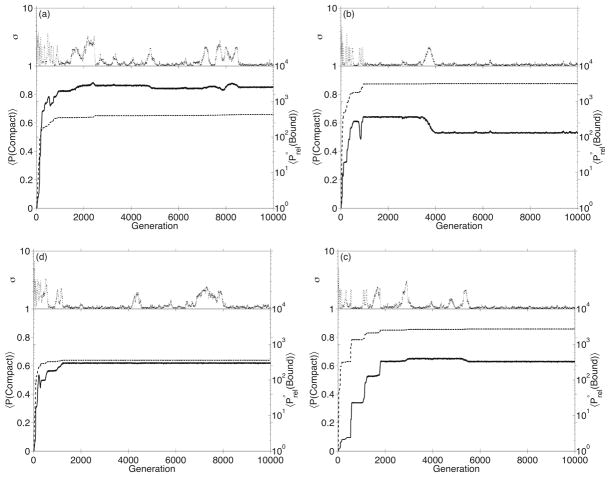
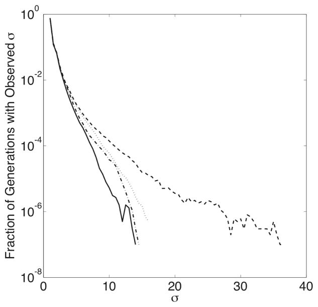
To study the effects of recombination in populations of evolving proteins, we perform several evolution experiments with different values of ρ: ρ = 0.0, 0.001, 0.01, and 0.1 recombination events per sequence per generation. Each experiment includes 1000 simulation runs of 10000 generations, with μ = 0.01. In Figure 1, we show the time-course of the population-weighted average folding and binding probabilities for several typical simulation runs. In general, the average binding probability rapidly increases in a punctuated fashion for several hundred generations, then fluctuates until the end of the simulation. This behavior is due to the relationship between fitness and $P_{\text{rel}}^{\circ }(\text{Bound})$ described in equation 7. Initially, when binding probabilities are low, proteins that bind comparatively better have a selective advantage and are more successful at replicating, raising the average binding probability. Later, when $\langle P_{\text{rel}}^{\circ }(\text{Bound})\rangle$ becomes very large, the selective advantage of higher binding probability saturates, so proteins become more equally fit, and random factors have a greater influence on the makeup of the population than fitness effects. 〈P(Compact) 〉 and $\langle P_{\text{rel}}^{\circ }(\text{Bound})\rangle$ generally (but not always) increase concomitantly. Figure 1 also shows the time-course of σ, a measure of population diversity defined as $\sigma ={({\sum }_s{(\frac{n_s}{N})}^2)}^{-1}$, where n_s is the number of copies of sequence s in the population. A population with only one unique sequence has a σ value of 1.0; a population where each sequence is different would have a σ value of N. As demonstrated by Figure 2, higher rates of recombination lead to more diverse populations, in agreement with the work by Cui and co-workers.⁹

Fig. 1.

Sample evolution runs from evolution experiments, showing the time-course of 〈P (Compact)〉 (solid lines), $\langle P_{\text{rel}}^{\circ }(\text{Bound})\rangle$ (dashed lines), and σ (dotted lines). Plots (a) and (b) are runs from experiments with ρ = 0.0, (c) and (d) are runs from experiments with ρ = 0.1.

Fig. 2.

The distribution of observed σ values in each set of simulation runs, graphed according to the value of ρ: ρ = 0.0 (solid line), ρ = 0.001 (dash-dot line), ρ = 0.01 (dotted line), and ρ = 0.1 (dashed line). Note that while the majority of observed σ values are quite low for any given value of ρ, the higest values of σ (and thus more diverse populations) are observed more frequently for higher values of ρ.

3.1. Conservative effects on sequence and fitness

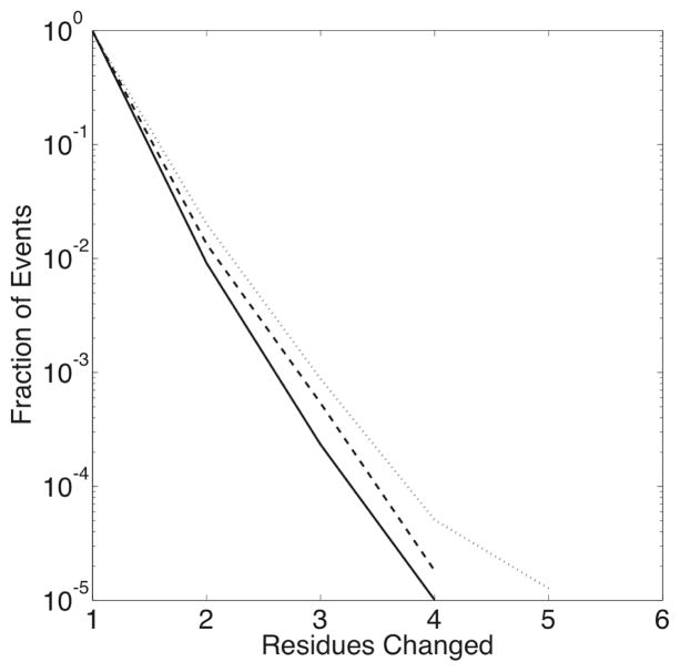
As simulated here, recombination generally has a limited effect on the protein sequence. The overwhelming majority of recombination events only affect at most one amino acid residue; the number of observed change events decreases exponentially as the number of residues changed increases, as shown in Figure 3. Mutation events change only one residue of the protein sequence, but proteins may experience more than one mutation per generation; however, such scenarios are also rare. No protein sequence experiences more than four mutation events per generation, and no recombination event changes more than five residues.

Fig. 3.

The observed fraction of recombination events changing a given number of sequence positions, measured over the entire 10, 000 generations of each of the 1, 000 simulations in each set, plotted for non-zero values of ρ: ρ = 0.001 (dash-dot line), ρ = 0.01 (dotted line), ρ = 0.1 (dashed line).

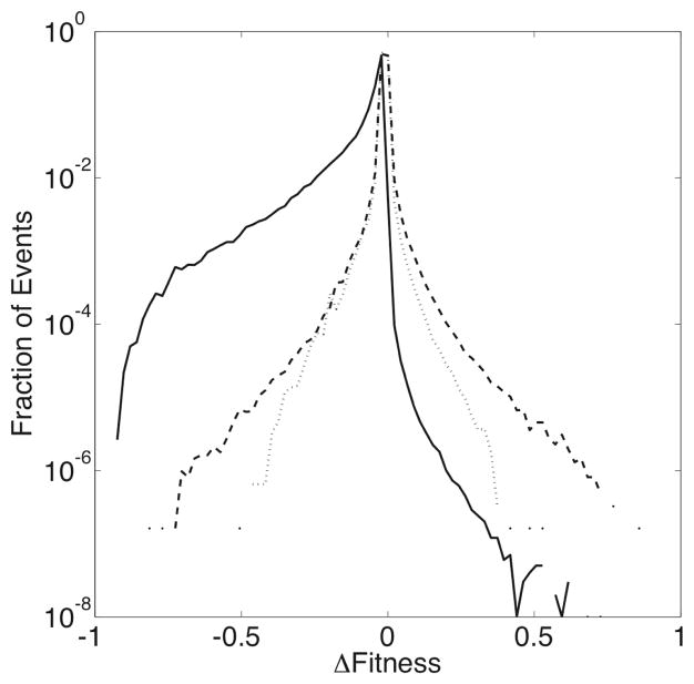
To compare how mutation and recombination affect the fitness of individual sequences, we measure the change in fitness resulting from each sequence change event in each experiment and plot the distribution of Δs values in Figure 4. The difference in fitness due to a mutation (Δs_mut) is simply defined as the fitness of the mutated sequence relative to its original form. Recombination involves two parent ({p₁, p₂}) and two daughter ({d₁, d₂}) sequences, so the definition of Δs is less straightforward. We calculate two different quantities in an attempt to capture the true character of the effects of recombination. We define $\mathrm{\Delta }{s}_{\text{rec}}^{max}$ as the difference in fitness between the most fit daughter and parent sequences: (max[s(d₁), s(d₂)] − max[s(p₁), s(p₂)]), and $\mathrm{\Delta }{s}_{\text{rec}}^{\text{avg}}$ as the change in the average fitness between the parents and daughters: $(\frac{s(d_1)+s(d_2)}{2}-\frac{s(p_1)+s(p_2)}{2})$.

Fig. 4.

The observed densities of Δs_mut (solid lines), $\mathrm{\Delta }{s}_{\text{rec}}^{max}$ (dashed lines), and $\mathrm{\Delta }{s}_{\text{rec}}^{\text{avg}}$ (dotted lines), the values of the change in fitness due to mutation, and the values of the change in maximum and average fitness due to recombination. These distributions are measured over the entire length of 10, 000 generations for each of the 1, 000 simulations in a set. For clarity, only the results from the experiment with ρ = 0.1 is shown. (The distributions are similar for experiments with different values of ρ.)

In agreement with previous theoretical models of protein sequence evolution,²⁴ the majority of mutation events have a minimal effect on fitness – small magnitude Δs values are much more common than larger values. As shown in Figure 4, however, mutations are deleterious far more often, and advantageous far less often than recombination. This is despite the fact that both processes most often result in the change of only one amino acid residue, but a significant number of events of each type change two residues (proteins can undergo several mutation events in each generation). The distributions of Δs_mut are asymmetric and skewed negative, which is likely due to the fact that the mutations are occuring in relatively-fit proteins. The smaller number of deleterious recombination events might represent the fact that recombination tends to swap relatively compatible amino acids, and might therefore tend to cause smaller changes in the fitness. It is surprising to note, then, that the probability of a beneficial change is significantly higher for recombination events, compared with simple mutations.

If the tendency for mutations to be deleterious is because of the relatively high fitness levels of the evolved sequences, we would expect that mutations would be more likely to be beneficial in the beginning generations of the simulations, before the fitness has increased to its equilibrium values. To test this, we measure the distributions of Δs_mut and $\mathrm{\Delta }{s}_{\text{rec}}^{max}$ in the first 500 and last 500 generations of an additional evolution experiment with 100 simulations with μ = 0.01, and ρ = 0.1. In the first 500 generations, where fitness values are relatively low, mutation events are indeed slightly more beneficial than in the final 500 generations, as shown in Figure 5. Interestingly the net fitness effects of recombination do not change –the distribution of $\mathrm{\Delta }{s}_{\text{rec}}^{max}$ for the last 500 generations is slightly broader but still symmetric. (Similar results are observed for the distributions of $\mathrm{\Delta }{s}_{\text{rec}}^{\text{avg}}$.) At all times in the simulation homologous recombination seems to result in a more favorable distribution of fitness changes than mutations.

Fig. 5.

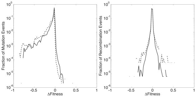
The observed distributions of Δs_mut and $\mathrm{\Delta }{s}_{\text{rec}}^{max}$ in the first and last 500 generations of experiments with ρ = 0.1. Solid lines represent the distributions corresponding to the first 500 generations of the experiment, dashed lines represent those corresponding to the final 500 generations. (a): Distribution of Δs_mut and (b): $\mathrm{\Delta }{s}_{\text{rec}}^{max}$.

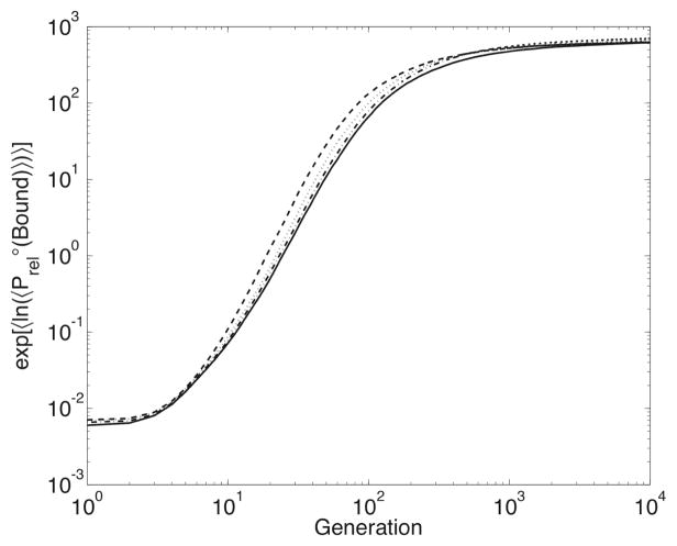
Mutation and recombination thus have different effects on the fitness at the level of the individual protein sequence, in spite of similar effects on the sequence itself. To determine if this affects the properties of evolving populations, we measure the time-course of $exp[\langle ln(\langle P_{\text{rel}}^{\circ }(\text{Bound})\rangle )\rangle ]$, the log-transformed relative binding probability averaged over all runs in an experiment. (The inner 〈 · · · 〉 represents the population-weighted average and the outer 〈 · · · 〉 represents the average over all simulations in the experiment. We measure this log-transformed average rather than the simpler $\langle \langle P_{\text{rel}}^{\circ }(\text{Bound})\rangle \rangle$, as the former is less susceptible to the influence of uncommonly-strong binding that occurs sporadically during some simulations.) The time-courses for each experiment are compared in Figure 6 The rate of recombination has an immediate effect on binding probability and fitness: within ten generations, the higher the value of ρ, the higher the value and rate of increase of $exp[\langle ln(\langle P_{\text{rel}}^{\circ }(\text{Bound})\rangle )\rangle ]$. This effect is short-lived – after approximately six hundred generations, the log-transformed average binding probabilities of the experiments with lower values of ρ catch up, and by the final generation, the binding probability distributions do not differ significantly. Higher rates of recombination are initially advantageous, but this advantage decreases over time, likely due to the nature of the fitness function and not due to any detrimental effects of recombination.

Fig. 6.

Time-course of the log-transformed average $exp[\langle ln(\langle P_{\text{rel}}^{\circ }(\text{Bound})\rangle )\rangle ]$, graphed according to the value of ρ: ρ = 0.0 (solid line), ρ = 0.001 (dash-dot line), ρ = 0.01 (dotted line), and ρ = 0.1 (dashed line).

3.2. The competitive advantage of higher recombination rates

To determine if higher rates of recombination can provide a competitive advantage, we perform a set of evolution experiments with two separate subpopulations whose sole initial difference is that recombination occurs between members of one sub-population only. Proteins in both subpopulations undergo mutation at equal rates (μ = 0.01). Although the combined total population size, remains at a constant 1000 proteins throughout the entire run, the size of each subpopulation may increase or decrease as a result of success at replication; offspring remain in the same subpopulation as the parent. In each generation, the number of recombination events taking place between proteins in the recombinant subpopulation (of size n_rec) is determined from a Poisson distribution with a mean of ρn_rec. We perform five experiments in this manner with 1000 simulation runs and 250 generations. Values of ρ in four experiments were 0.001, 0.01, 0.1 and 1.0 recombination events per sequence per generation. In a fifth, control experiment, ρ = 0.0, so no recombination takes place, and n_rec changes at random.

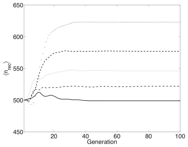
We plot the average value of n_rec for each generation of each experiment in Figure 7. The strength of selection is strong enough that within 100 generations, the entire population is made up exclusively of members of one subpopulation. Therefore, only in the initial generations can 〈n_rec 〉 be treated as an actual average subpopulation size; by generation 100, 〈n_rec 〉 is more accurately described as the number of simulations in which the recombining subpopulation has become fixed. The subpopulation in which a highly fit sequence first appears has a great advantage. When neither subpopulation undergoes recombination (ρ = 0.0), each subpopulation has an equal chance of producing this new sequence. This means that each subpopulation is equally-likely to take over, which is reflected in the final 〈n_rec〉 value of 499 for the control experiment. However, due to the faster increase in fitness in recombining populations demonstrated in Figure 6, beneficial mutations are more likely to arise in a population undergoing recombination; these subpopulations are more likely to out-complete mutation-only subpopulations. The higher the value of ρ, the better they compete, as shown in Figure 7. This effect is even more dramatic for larger population sizes. In an experiment with N = 10000 sequences and ρ = 1.0, the recombinant subpopulation ultimately dominates in 86% of the simulations. Recombination, at least initially, provides a competitive advantage, that may become fixed in the resulting population.

Fig. 7.

Time-course of 〈n_rec〉, the experimental-wide average size of the subpopulation with recombination, color-coded by the value of ρ. The control experiment without recombination, ρ = 0.0 (solid line), ρ = 0.001 (dash-dot line), ρ = 0.01 (dotted line), ρ = 0.1 (dashed line), ρ = 1, (large dots).

4. Conclusion

In agreement with the neutral theory of evolution, most observed mutations affect fitness only slightly, or are detrimental.²⁴ Large decreases in fitness due to mutation are observed and are comparable with the loss of a structurally-important or active site residues. Recombination events are, on average, more likely to be beneficial than mutation events. There are different reasons why recombination might provide a selective advantage, such as the possibility that recombination events exploring novel, more fit sequences, as Cui et al. suggest,⁹ or that recombination events hasten the adoption of already discovered optimal sequences, as suggested by Xia and Levitt.¹¹

Even though the distribution of advantageous and deleterious recombination events does not significantly change during the simulation, the benefit of recombination on the average fitness of the population is greatest early in evolutionary runs when fitness values are comparatively low, providing no real increase in final fitness values. This is akin to the idea of Fitness Associated Recombination,²⁵ an increase in the rate of recombination correlated with an era of lower fitness. This selective advantage of recombining populations – although short-lived – can result in fixation of a high recombination rate in the population. In this case, the presence of exons, increasing the recombination rate in real proteins, might have arisen for the advantages that it conferred during the early stages of evolution. If so, other advantages of exons, such as (for example) alternative splicing, might have arisen later, taking advantage of the already-present exonic structure.

These simulations involve short sequences and limited genetic diversity, suggesting more interesting results may be found by studying longer sequences and more diverse populations. Longer sequences may be expected to be more robust to genetic change, suggesting that even greater amounts of mutation and especially recombination may be tolerated.

References

- 1.Wagner GP, Altenberg L. Evolution. 1996;50:967. doi: 10.1111/j.1558-5646.1996.tb02339.x. [DOI] [PubMed] [Google Scholar]
- 2.Kirschner M, Gerhart J. Proc Natl Acad Sci USA. 1998;95:8420. doi: 10.1073/pnas.95.15.8420. [DOI] [PMC free article] [PubMed] [Google Scholar]
- 3.Bedau MA, Packard NH. Biosystems. 2003;69:143. doi: 10.1016/s0303-2647(02)00137-5. [DOI] [PubMed] [Google Scholar]
- 4.Earl DJ, Deem MW. Proc Natl Acad Sci USA. 2004;101:11531. doi: 10.1073/pnas.0404656101. [DOI] [PMC free article] [PubMed] [Google Scholar]
- 5.Sambrook J. Nature (London) 1977;268:101. doi: 10.1038/268101a0. [DOI] [PubMed] [Google Scholar]
- 6.Gilbert W. Nature (London) 1978;271:501. doi: 10.1038/271501a0. [DOI] [PubMed] [Google Scholar]
- 7.Gilbert W. Cold Spring Harbor Symp Quant Biol. 1987;52:901. doi: 10.1101/sqb.1987.052.01.098. [DOI] [PubMed] [Google Scholar]
- 8.Bogarad LD, Deem MW. Proc Natl Acad Sci USA. 1999;96:2591. doi: 10.1073/pnas.96.6.2591. [DOI] [PMC free article] [PubMed] [Google Scholar]
- 9.Cui Y, Wong WH, Bornberg-Bauer E, Chan HS. Proc Natl Acad Sci USA. 2002;96:2591. doi: 10.1073/pnas.022240299. [DOI] [PMC free article] [PubMed] [Google Scholar]
- 10.Cebrat S. Int J Mol Phys C. 2005 in press. [Google Scholar]
- 11.Xia Y, Levitt M. Proc Natl Acad Sci USA. 2002;99:10382. doi: 10.1073/pnas.162097799. [DOI] [PMC free article] [PubMed] [Google Scholar]
- 12.Chan HS, Bornberg-Bauer E. Applied Bioinformatics. 2002;1:121. [PubMed] [Google Scholar]
- 13.Bornberg-Bauer E. Biophys J. 1997;73:2393. doi: 10.1016/S0006-3495(97)78268-7. [DOI] [PMC free article] [PubMed] [Google Scholar]
- 14.Bornberg-Bauer E, Chan HS. Proc Natl Acad Sci USA. 1999;96:10689. doi: 10.1073/pnas.96.19.10689. [DOI] [PMC free article] [PubMed] [Google Scholar]
- 15.Xia Y, Levitt M. Proteins. 2004;55:107. doi: 10.1002/prot.10563. [DOI] [PMC free article] [PubMed] [Google Scholar]
- 16.Hirst JD. Protein Eng. 1999;12:721. doi: 10.1093/protein/12.9.721. [DOI] [PubMed] [Google Scholar]
- 17.Blackburne BP, Hirst JD. J Chem Phys. 2001;115:1935. doi: 10.1063/1.2056545. [DOI] [PubMed] [Google Scholar]
- 18.Blackburne BP, Hirst JD. J Chem Phys. 2003;119:3453. doi: 10.1063/1.2056545. [DOI] [PubMed] [Google Scholar]
- 19.Williams PD, Pollock DD, Goldstein RA. J Mol Graph Modell. 2001;19:150. doi: 10.1016/s1093-3263(00)00125-x. [DOI] [PMC free article] [PubMed] [Google Scholar]
- 20.Bloom JD, Wilke CO, Arnold FH, Adami C. Biophys J. 2004;86:2758. doi: 10.1016/S0006-3495(04)74329-5. [DOI] [PMC free article] [PubMed] [Google Scholar]
- 21.Miyazawa S, Jernigan RL. Macromol. 1985;18:534. [Google Scholar]
- 22.Govindarajan S, Goldstein RA. Proc Natl Acad Sci USA. 1998;95:5545. doi: 10.1073/pnas.95.10.5545. [DOI] [PMC free article] [PubMed] [Google Scholar]
- 23.Irbäck A, Troein C. J Biol Phys. 2002;28:1. doi: 10.1023/A:1016225010659. [DOI] [PMC free article] [PubMed] [Google Scholar]
- 24.Taverna D, Goldstein RA. J Mol Biol. 2002;315:479. doi: 10.1006/jmbi.2001.5226. [DOI] [PubMed] [Google Scholar]
- 25.Hadany L, Beker T. J Evol Biol. 2003;16:862. doi: 10.1046/j.1420-9101.2003.00586.x. [DOI] [PubMed] [Google Scholar]