Treatment selections using risk–benefit profiles based on data from comparative randomized clinical trials with multiple endpoints

Abstract

In a typical randomized clinical study to compare a new treatment with a control, oftentimes each study subject may experience any of several distinct outcomes during the study period, which collectively define the “risk–benefit” profile. To assess the effect of treatment, it is desirable to utilize the entirety of such outcome information. The times to these events, however, may not be observed completely due to, for example, competing risks or administrative censoring. The standard analyses based on the time to the first event, or individual component analyses with respect to each event time, are not ideal. In this paper, we classify each patient's risk–benefit profile, by considering all event times during follow-up, into several clinically meaningful ordinal categories. We first show how to make inferences for the treatment difference in a two-sample setting where categorical data are incomplete due to censoring. We then present a systematic procedure to identify patients who would benefit from a specific treatment using baseline covariate information. To obtain a valid and efficient system for personalized medicine, we utilize a cross-validation method for model building and evaluation and then make inferences using the final selected prediction procedure with an independent data set. The proposal is illustrated with the data from a clinical trial to evaluate a beta-blocker for treating chronic heart failure patients.

1. Introduction

Consider a randomized, comparative clinical trial in which a treatment is assessed against a control with respect to their risk–benefit profiles. For each study patient, the outcome variables include a set of distinct event time observations reflecting such profiles during the study period. Often these event times cannot be observed completely due to the presence of competing risks. For example, to investigate if the beta-blocking drug bucindolol would benefit patients with advanced chronic heart failure (HF), a clinical trial, “Beta-Blocker Evaluation of Survival Trial” (BEST), was conducted (BEST, 2001). There were 2708 patients enrolled and followed for an average of 2 years. The primary endpoint of the study was the patient's overall survival time. The -value based on the standard two-sample log-rank test was 0.10, with a corresponding hazard ratio estimate of 0.90 (95% CI: 0.78–1.02), numerically favoring the beta-blocker. Although mortality is an important endpoint, the evaluation of treatment benefit should also include morbidity for chronic HF patients. One important morbidity measure is the time to hospitalization, especially due to worsening HF, which may be censored by the patient's death. To avoid such competing-risk problems with multiple outcomes, conventionally we consider the time to the first among several events as the endpoint. For example, for the “BEST” study, the competing events are death and HF or non-HF hospitalization. With this composite endpoint, the log-rank -value is 0.14, with a corresponding hazard ratio estimate of 0.93 (95% CI: 0.85–1.02). Note that this type of endpoint does not fully reflect the disease burden or progression over the patient's follow-up, since only one event at most is utilized per patient, and its interpretation is further complicated by combining events of differing levels of severity into a single outcome. In Table 1, we show the frequencies of the occurrences of these component endpoints from the study patients whose data were obtained from the National Heart, Lung, and Blood Institute (NHLBI). Note that mortality may be classified as either cardiovascular (CV) or non-CV related. In general, it is not expected that a beta-blocker would have any beneficial effect on non-CV outcomes. In addition, part of any undesirable side effects of the beta-blocker may be captured by, for example, non-CV related death or non-HF hospitalization.

Table 1.

Numbers of patients experiencing specific clinical endpoints in control and treatment groups in BEST

Outcome	Control	Treated
Any event	971	930
Death	448	411
CV death	388	342
Non-CV death	60	69
Any hospitalization	874	829
HF hospitalization	568	476
Non-HF hospitalization	634	619
Total patients	1353	1354

CV, cardiovascular; HF, heart failure.

For a typical CV study like BEST with multiple event time observations, conventional secondary analyses for risk–benefit assessments are often conducted with respect to each individual endpoint (for example, the time to HF hospitalization). The conclusions of such component analyses can be misleading due to competing risks. Among other limitations, because component events are analyzed separately rather than jointly, they ignore any relationship between the timing and occurrence of different types of events at the patient level and cannot provide a global, clinically meaningful evaluation of the new treatment (Claggett and others, 2013). There are novel procedures for handling multiple event time observations proposed, for example, by Andersen and Gill (1982), Wei and others (1989), and Lin and others (2000). In the presence of competing risks, however, the above procedures or their modifications are not entirely satisfactory for assessing the treatment's overall risk and benefit (Li and Lagakos, 1998; Ghosh and Lin, 2003; Pocock and others, 2012).

In this article, we propose an ordinal categorical outcome variable which reflects the individual patient's morbidity, including toxicity, as well as mortality over a specific time period for evaluating and comparing the treatments. For example, for the BEST study, with guidance from our cardiologist co-author, we classified patient response, using eight ordinal categories, based on the disease burden during the first 18 months of follow-up. This time point was chosen for illustration due to the noted concerns over potentially harmful early effects associated with initial dosing and upward titration of the study drug, and represents the minimum anticipated follow-up time for enrolled patients according to the initial study design (BEST, 2001). We also consider analyses using the anticipated average follow-up time for the BEST study, 36 months. Category 1 is assigned if the patient has experienced neither death nor any hospitalization prior to the time of evaluation. A patient is classified as Category 2 if he or she is alive and has experienced only non-HF hospitalization (reflecting potential toxicity). Categories 3 and 4 denote patients who are alive, but have experienced a single (Category 3) or recurrent (Category 4) instance of HF hospitalization. Categories 5 through 8 are assigned to patients who died during follow-up, with a distinction made between “early” or “late” death (i.e. before or after 12 months) as well as cause of death. The relative ordering is as follows: late non-CV death (Category 5), late CV death (Category 6), early non-CV death (Category 7), and early CV death (Category 8). Note that some study patients might not have their entire clinical history, until their time of death or at 18 months after randomization, available due to non-informative, or administrative, censoring.

In the paper, we first present methods for analyzing such ordinal data, possibly incomplete due to non-informative censoring, in a two-sample overall comparison setting. To bring the clinical trial results to the patient's bedside, we may utilize the patient's baseline characteristics to perform personalized or stratified medicine. Here, we present a systematic approach to create a scoring system using the patient's multiple baseline covariates and utilize this system to stratify the patients for evaluation with respect to the ordinal categorical outcomes. More specifically, to avoid overly optimistic model selections, we first divide the data set into two pieces. The two pieces may be obtained by splitting the entire data set randomly. With the first piece, a cross-validation procedure is utilized to select the best scoring system among all of the competing models of interest for ordinal categorical data. We then use the second piece (the so-called holdout sample) to make inferences about the treatment differences over a range of the score selected from the first stage. All proposals are illustrated with the data from the BEST study.

When there is a single baseline covariate involved Song and Pepe (2004), and Bonetti and Gelber (2004) have proposed novel statistical procedures for identifying a subgroup of patients who would benefit from the new treatment with respect to a single outcome. A recent paper by Janes and others (2011), based on previous work by Huang and others (2007), and Pepe and others (2008), provides practical guidelines for assessing the performance of individual markers for the purposes of treatment selection. By incorporating more than one baseline covariate, our approach is similar in spirit to Cai and others (2011) and Li and others (2011). However, they used the data from the entire study to create a scoring system, for a single outcome or for a single treatment group only, by fitting a prespecified model without involving model evaluation or variable selection and then used the same data set to make inferences. Our proposal explores so-called “personalized” treatment effects in the presence of multiple time-to-event outcomes and explores the properties of an ordinal classification scale derived from multiple, partially censored event times.

2. Two-sample assessment of treatment using incomplete categorical data

For the th patient in the th treatment group (; ), let be the time to the first occurrence of a terminal event from among the competing risks of interest. Note that may be infinite if there is no terminal event. Let be the independent censoring variable for with survival function . Let the minimum of and and where is the indicator function. For each study patient, assume that based on his/her entire morbidity and mortality endpoint information up to time , where pr, one can classify the outcome as one of ordered categories, ordered from “best” to “worst”. Note that we do not require traditional “competing risks” methods to account for informative censoring because we include such informative events in the definition of the outcome categories.

Noting that a patient's outcome status is fully observable when , the cumulative cell probabilities can be consistently estimated by the inverse probability of censoring weighting (IPCW) estimator

(2.1)

where and is the Kaplan–Meier estimator for (Li and others, 2011). It follows that the cell probability can be estimated by , where . Note that the information regarding the events observed prior to the censoring time is completely ignored in (2.1) and the resulting IPCW procedure may not be “efficient”. For example, for the BEST study, a subject who experienced a single HF hospitalization prior to censoring, must have at time , even though the specific value of at may not be known due to censoring. To characterize this kind of information, let be the earliest time at which the value is determined. For example, with the data from BEST, let , and be the first non-HF, first HF, and second HF hospitalization times, respectively. It follows that , , , and . With this additional information, a more efficient estimator for the can be obtained by replacing the weight in (2.1) with

(2.2)

where is the Kaplan–Meier estimator for using paired observations . Note that with small sample sizes, some 's may be negative due to random variation. In such a case, one may utilize the conventional, simple iterative pool adjacent violator algorithm (Ayer and others, 1955). Unless otherwise specified, we employ weights for the remainder of the paper.

In order to compare two treatment groups with such ordinal categorical outcomes, one may compare the cumulative distributions . Let and be the corresponding estimators. Note that each value may be interpreted as the risk difference with respect to a binary outcome in which “success” is defined by a patient experiencing . To make inferences on the difference of these two distribution functions, we may use bootstrapping or perturbation-resampling methods (Uno and others, 2007). Details are provided in Appendix A of supplementary material available at Biostatistics online. For the data from BEST, let months. Table 2 displays the profiles of the estimated distribution functions for each treatment group using weights (2.2), and indicating that the beta-blocker group is better than its control counterpart with respect to each outcome.

Table 2.

Estimated distribution functions for control and treated groups with BEST data with months

	Control ()		Treated ()		Contrast ()
Outcome category		pr()		pr()	Est	SE
1	397	0.38	442	0.41	0.04	0.02
2	174	0.54	224	0.62	0.08	0.02
3	120	0.66	102	0.72	0.06	0.02
4	131	0.78	88	0.80	0.03	0.02
5	11	0.78	17	0.82	0.03	0.02
6	83	0.86	58	0.87	0.01	0.01
7	24	0.87	22	0.88	0.01	0.01
8	163	1.00	153	1.00	–	–
(censored)	250	–	248	–	–	–

To compare two groups with respect to ordinal categorical outcomes, a conventional way to summarize the treatment difference is to use an ordinal regression model. Let for patients in the active treatment group and otherwise, then this model is where is a known, increasing function, , and and are unknown parameters. Even if the model is not correctly specified, a that significantly differs from 0 can be used as evidence of the superiority of one treatment relative to the other. For the present case, a negative value for corresponds to a reduction in overall “risk” associated with treatment. With censored observations, the treatment difference can be estimated by maximizing the weighted multinomial log-likelihood function:

(2.3)

where and standard error estimates can be obtained analytically. Under mild conditions, the estimator from the above model converges to a finite constant as even when the model is not correctly specified (Zheng and others, 2006; Uno and others, 2007; Li and others, 2011). For the data from BEST, when is the logit function, is 0.204 with a standard error estimate of 0.074. This indicates that the beta-blocker indeed reduces the disease burden. Details are given in Appendix A of supplementary material available at Biostatistics online.

Rather than using a parametric summary of the treatment difference which may not be easily interpretable unless the model is correctly specified, an intuitively interpretable, non-parametric summary measure is the so-called general risk difference, which has been studied extensively as an extension of the simple risk difference for ordinal data (Agresti, 1990; Edwardes, 1995; Lui, 2002). In this setting, the general risk difference, which is closely related to Wilcoxon's rank-sum statistic, is , where , , is a patient response randomly chosen from treatment group , with positive values suggesting that patients receiving active treatment are more likely to be “healthier” than their independent control counterparts .

A consistent estimator for then is where . The standard error estimate can be obtained by perturbation-resampling methods as in Uno and others (2007). For the data from the BEST trial, with standard error estimate of , suggesting a net 6.4% probability of improved health associated with active treatment. Using this model-free summary of the treatment difference, the beta-blocker again appears better than the control. Details are given in Appendix A of supplementary material available at Biostatistics online. As a sensitivity analysis, we considered a condensed, five-category classification system in which recurrent HF hospitalizations are ignored and no distinction is made between early and late death. Despite more crudely categorizing patients, the results are quite similar, still significantly favoring the beta-blocker group: and .

3. Construction and selection of a patient-level stratification system

Suppose that is the baseline covariate vector for a subject randomly chosen from the th treatment group . Our goal is to make inference about the treatment difference based on and , conditional on , any given value in the support of the covariate vector. Ideally, one would estimate this conditional treatment difference via a non-parametric procedure. However, if the dimension of is greater than 1, it seems difficult, if not impossible, to do so. A practical alternative is to model the relationship between the treatment difference and parametrically and then evaluate the prediction performance of the final selected model. To avoid an ‘overly optimistic’ prediction model, we split the data set into two pieces, say, part A and part B. With the data from part A, we build various candidate models for the treatment differences and evaluate them via a cross-validation procedure. This results in a univariate scoring system with which to stratify the patients, referred to here as a treatment selection score. In this section, we present the first step using the part A data, i.e. the construction and selection of the scoring system, and in the next section, we show how to make inferences about the treatment differences based on the selected scoring system using the part B data.

It is important to note that, to validate the scoring system, we need a model-free summary measure for the treatment difference. For the present case with the ordinal categorical response discussed in Section 2, the treatment contrast,

(3.1)

is model-free and heuristically interpretable. Note also that to obtain a coherent prediction system, it is preferable to use the same treatment contrast measure for model building, selection and validation.

3.1. Creating treatment difference scoring systems

In order to estimate (3.1) parametrically, one can model the ordinal categorical response via two separate ordinal regression models, that is, for each treatment and conditional on :

(3.2)

where , is a function of , is a known monotone increasing function, and and are unknown parameters. It follows that a parametric estimate for is given by

(3.3)

where estimated probabilities are obtained from the fitted models (3.2) and , with , . Alternatively, we may use a single model

(3.4)

to obtain estimates where = , and , and are unknown parameters. Models (3.2) and (3.4) may be fitted by maximizing the corresponding inverse probability weighted log-likelihood functions with IPC weights or . Under mild conditions, the resulting estimators of model parameters converge to a finite constant vector as even when the model (3.2) or (3.4) is not correctly specified (Uno and others, 2007).

3.2. Evaluation and selection of a final model for stratification

To choose the “best” stratification system from among all candidate working models, we evaluate the models using a cross-validation procedure. Specifically, we split the data into two parts randomly. We fit the data from the first part with each of the working models, then use the data from the second part to evaluate them based on (3.1). Unlike the one-sample risk prediction problem, most standard evaluation criteria based on individual prediction errors are not applicable here because no measure of treatment difference is observable at the patient level. However, a “goodness of fit” measure using the concordance between the true, unobservable treatment difference in (3.1) and the rank of the parametric predicted treatment difference , say, , can be estimated consistently under the current setting, where is the distribution function of and the covariance is with respect to the random covariate vector . Here, can be estimated by where is the ICPW estimator for based on subjects with is the empirical cumulative distribution function of . Justification of the consistency of can be derived using similar arguments to those given by Zhao and others (2013). Since the variances of and are independent of the fitted model, the correlation corresponding to can be estimated up to a common constant across all candidate models. Therefore, to quantify the improvement of, say, Model I relative to Model II, we may take the ratio of the resulting covariance estimates to estimate the ratio of the two corresponding correlation coefficients , to guide model selection.

We use a repeated random cross-validation procedure, in each iteration randomly dividing this part A data set into two mutually exclusive subsets, and , the “model building set” and “evaluation set”, respectively. For each model building procedure, we can construct a model, using only data in to obtain via (3.3), then compute all , for all in . We repeatedly split the training data set times. For each , and for each modeling procedure, we obtain an estimate of the concordance . Lastly, we average these estimates over to obtain final estimates . The modeling procedure which yields the largest cross-validated values will be used for the construction of our final working model. We then refit the entire part A data set with this specific modeling procedure in order to construct the final score.

3.3. Construction and selection of scoring systems using the BEST data set

To illustrate the above model building and evaluation process with the data from BEST, we first split the data set into parts A and B, using the first 900 () patients according to their randomly assigned Study ID number as part A and using the remaining patients as part B. Note that Shao (1993) presents theoretical justifications for the preference of a relatively large holdout sample, and a comparatively smaller sample size devoted to “model construction”.

Here the covariate vector consists of 16 clinically relevant covariates from Castagno and others (2010, Table 1). These baseline variables are: age, sex, left ventricular ejection fraction (LVEF), estimated glomerular filtration rate (eGFR) adjusted for body surface area, systolic blood pressure (SBP), class of HF (Class III vs. Class IV), obesity (body mass index 30 vs. 30), resting heart rate, smoking status (ever vs. never), history of hypertension, history of diabetes, ischemic HF etiology, presence of atrial fibrillation, and race (white vs. non-white). As in Castagno and others (2010), we used 3 indicator variables to discretize eGFR values into 4 categories, with cut-points of 45, 60, and 75.

Models (3.2) and (3.4) were utilized with the logit and complementary log–log links, , respectively. For each of type of model, we estimated the model parameters using IPC weights and . For illustration, a total of eight modeling procedures were considered in our analysis.

To evaluate these models, we used a repeated random cross-validation procedure with of the part A data used for model building and for evaluation with iterations. In Table 3, we present these modeling procedures along with their relative concordance value, based on with the modeling approach of separate logistic regression models (logit link), with “complete-case” weights (), as the reference model.

Table 3.

Multinomial model building procedures with average cross-validated concordance values

Separate/single models	Link	Weighting scheme	ratio
Separate	Logit		(ref)
Separate	Logit		2.81
Separate	c-log–log		2.63
Separate	c-log–log		3.16
Single	Logit		0.94
Single	Logit		2.88
Single	c-log–log		2.63
Single	c-log–log		3.23

Indicates the largest value, and therefore the selected optimal model building procedure.

The model found to provide the greatest concordance was the interaction model with the complementary log–log link function fitted using . The resulting model and bootstrapped standard errors (SE) with the selected best model building procedure are given in Table 4.

Table 4.

Regression coefficient estimates and standard errors (SE) from the final working model using BEST training data with link function

Covariate	Main effects	Treatment interaction terms
Age	0.000 (0.006)	0.006 (0.009)
Male	0.064 (0.139)	0.095 (0.199)
LVEF	0.017 (0.008)	0.016 (0.012)
I(eGFR 75)	0.011 (0.166)	0.470 (0.216)
I(eGFR 60)	0.049 (0.161)	0.059 (0.238)
I(eGFR 45)	0.692 (0.165)	0.032 (0.229)
SBP	0.014 (0.003)	0.009 (0.005)
Class IV HF	0.292 (0.196)	0.499 (0.277)
I(BMI 30)	0.157 (0.127)	0.031 (0.193)
Ever smoker	0.090 (0.114)	0.214 (0.176)
Heart rate	0.005 (0.005)	0.011 (0.007)
History of hypertension	0.248 (0.130)	0.216 (0.180)
History of diabetes	0.251 (0.129)	0.228 (0.173)
Ischemic etiology	0.069 (0.137)	0.188 (0.183)
Atrial fibrillation	0.185 (0.181)	0.113 (0.231)
White race	0.043 (0.122)	0.145 (0.188)

4. Inferences about the treatment differences using the holdout sample

Let be the observed score, obtained from the part A data set, for a patient in the part B data set with covariates . In this section, using the data from part B, we make inferences about the general risk difference and the cumulative risk differences , where is outcome of a random patient in treatment group from a future population identical to the part B data. Rather than using a parametric estimate for these contrast measures, we use a non-parametric kernel functional estimation procedure conditional on the treatment selection score. To this end, let the conditional cell probabilities for the ordinal response be denoted by and cumulative probabilities by . Here is the sample size in the th group in the part B data set. The kernel estimators for are

where and are their counterparts from the part B data, is a smooth symmetric kernel with finite support and is a smoothing parameter. Lastly, can be estimated as , ; .

The resulting estimator for is . When , it follows from a similar argument by Li and others (2011) that converges to uniformly over , which is an interval within the support of . Consequently, for a fixed , converges in distribution to a normal with mean and variance as . Similarly, converges in distribution to a normal with mean and variance as . To approximate the distributions above, we use a perturbation-resampling method, which is similar to “wild bootstrapping” (Wu, 1986; Mammen, 1993) and has been successfully implemented in many estimation problems (Lin and others, 1993; Cai and others, 2010). In addition, () simultaneous confidence bands for and over can be obtained accordingly. Details are provided in Appendix B of supplementary material available at Biostatistics online.

As with any non-parametric estimation problem, it is important that we choose appropriate smoothing parameters in order to make inference about the treatment differences. Here, we may use the cross-validation method aiming for maximizing the weighted multinomial log-likelihood function as in Li and others (2011). Furthermore, to ensure the bias of the estimator is asymptotically negligible in the above large-sample approximation, however, we slightly undersmooth the data and obtain the final smoothing parameter by multiplying the cross-validation selected bandwidth with where is a small positive number less than 0.3.

Now, we apply the final scoring system derived from the part A data set to the patients in the part B data set mentioned in Section 3.3. We note that 63% of the estimated scores are greater than , indicating a model-based anticipated treatment benefit for a majority of patients.

For all kernel estimators, we let be the standard Epanechnikov kernel, with the chosen smoothing parameters , . The resulting estimates of the patient-specific treatment differences , with pointwise and simultaneous confidence interval estimates, are displayed in Figure 1. Using the final score derived from the model in Table 4 over the range , we find for and for . The point and interval estimates displayed in Figure 1 are quite informative for identifying subgroups of patients who would benefit from the beta-blocker with various desired levels of treatment differences. In particular, patients with scores 0.09 and 0.18 are found to experience significant treatment benefits (via the 95% confidence intervals and bands, respectively). In Appendix C of supplementary material available at Biostatistics online, we show the corresponding treatment differences with respect to the cumulative outcome probabilities . Note that each value allows for the estimation of the treatment contrast with respect to a different composite outcome. For example, refers to the effect of treatment on the composite outcome “any hospitalization or death”, as in the typical time to first event analysis. It can be seen that for and for , indicating that our score is also informative for identifying patients who would experience “treatment success” with respect to this outcome as well. Furthermore, using and , patients with scores 0.14 and 0.16 are found to experience significant treatment benefits via the 95% simultaneous confidence bands with respect to the desirable outcomes (alive with no HF hospitalization) and (alive with no recurrent HF hospitalization), respectively. Finally, we note that the estimated effects of treatment with respect to both death, , and early death, , are relatively constant across the range of scores.

Figure 1.

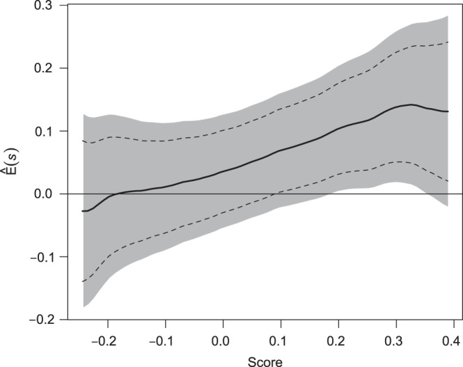
Estimated BEST treatment effect using treatment selection score presented in Table 4. Solid curve represents point estimates, with pointwise and simultaneous confidence intervals denoted by dashed lines and shaded region, respectively.

As an additional analysis, we also considered analyzing 36-month outcomes, which represents the initially planned average patient follow-up time (BEST, 2001). Despite noticeably higher rates of censoring (and a larger standard error), the two-sample analysis finds a similarly sized benefit for the treatment group overall. Using the same scoring system derived above to assess personalized treatment differences at 36 months resulted in both an increase in uncertainty for patient-specific estimates as well as a noticeably weaker association between the score and treatment effect estimates over the range of scores. As mentioned in Section 1, it is likely that “risk–benefit” effects of treatment are more heterogeneous and/or predictable at earlier time points in this setting, as they are associated with initial dosing procedures of the study drug. Results for this 36-month analysis are given in Appendix D of supplementary material available at Biostatistics online.

5. Simulation study

In order to examine the potential benefit of including multiple clinical endpoints in comparing treatments under practical settings, we conducted an extensive simulation study. For example, in one of the settings, we mimic the BEST study to generate multiple event time data. Specifically, we first fit a shared frailty model, using a parametric Weibull distribution (Rondeau and others, 2007) to the observed hospitalization data for each group, utilizing all covariates mentioned in Section 3.3 to estimate subject-specific scale parameter in BEST data, with a common shape parameter in each arm. For each simulated data set, we randomly generate 2707 new sets of times to fatal and non-fatal events from Weibull distributions using patient-level covariates drawn with replacement from the BEST study population. The Weibull shape parameters, from fitted estimates, used in simulations were for fatal events and and for non-fatal events in control and active treatment groups, respectively. These models produce fatal and non-fatal events that occur at a rate of 25.6 and 72.1 per 100 patient-years during the first 18 months after randomization in the control group. The corresponding rates in the treatment group were 24.2 (rate ratio ) and 64.1 (rate ratio ), respectively (Scenario 1). We then considered scenarios in which the treatment effect for death was strengthened to induce rate ratios of 0.90 (Scenarios 2 and 3) and 0.85 (Scenario 4), and similarly, the rate ratios for non-fatal events were improved to 0.85 (Scenarios 3 and 4). We also considered a global “null” scenario in which there was no treatment difference with respect to any outcome. We generated 200 simulated data sets for each scenario. Results corresponding to each of these scenarios are shown in Table 5.

Table 5.

Simulation results comparison of the usage of proposed multiple-outcome methods vs. traditional single-outcome methods with respect to two-sample power and identification of patient-level treatment response

			Two-sample power
	Incidence rate ratio		Multiple events	First composite event		Stratification score
	Fatal	Non-fatal	(%)	(%)	Log-rank (%)	Multinomial	Binomial	ratio
Global null	1	1	6	6	4	0.007	0.005	–
Scenario 1	0.95	0.89	34	24	6	0.018	0.014	1.30
Scenario 2	0.90	0.89	60	32	7	0.016	0.013	1.21
Scenario 3	0.90	0.85	69	39	16	0.016	0.013	1.22
Scenario 4	0.85	0.85	88	48	23	0.014	0.012	1.15

We first compare the two-sample performance of our proposed , which uses the proposed ordinal scale incorporating the complete clinical history to evaluate patients status at relative to standard procedures which use only the time to first clinical event up to based on (corresponding to the -year event rate), as well as the log-rank test. The new test based on is more powerful than the standard procedures. For example, in Scenario 4, the new test has 88% power, compared with 48% using the -year event rate and 23% for the log-rank test. The log-rank test is likely to be underpowered in all settings due to violation of the proportional hazards assumption. In order to compare the ability to appropriately identify patient-level treatment responses and stratify patients accordingly, we compared the ordinal logistic regression model chosen in Section 3.3 to a similar binary logistic regression model that used only the occurrence of the first composite event Cai and others (2011). Using 10-fold cross-validation in each simulated data set, we find that the ratio in each scenario, indicating the superiority of the stratification score obtained through the usage of the ordinal regression model. The corresponding averaged curves , as well as further details regarding the simulation setting, and model accuracy and classification, are provided in Appendix E of supplementary material available at Biostatistics online.

6. Remarks

The proposed procedures can be applied to any study with multiple endpoints which reflect a patient's risk–benefit profile. For example, a longitudinal trial may collect repeated measurements for an endpoint over time. The standard analysis, for example, via generalized estimating equations techniques (Liang and Zeger, 1986) provides a treatment comparison using an overall average mean difference of a response variable. Such a contrast may not be a sufficient summary, particularly when the temporal profile of such repeated measures should be considered for the outcome. One may instead classify the repeated measure profile for each patient into several clinically meaningful categories, such as those presented in this paper for evaluating the treatment's risk(s) and benefit(s) together.

In this article, we focus on a single assessment of patient outcomes using clinical outcomes occurring prior to the specific time point of interest. Future research is needed to better understand and analyze data arising from scenarios where differences in treatment effect may be related to the choice of follow-up time as well as baseline covariates, which may be encountered, for example, during interim monitoring of trials. For comparing scoring systems constructed for the treatment difference, we use a concordance measure between the observed and expected treatment differences. More research is needed to explore if other measures, which may be more clinically interpretable, can be used for model evaluation and selection.

Supplementary material

Supplementary Material is available at http://biostatistics.oxfordjournals.org.

Funding

This research was partially supported by US NIH grants and contracts (R01 AI052817, RC4 CA155940, U01 AI068616, UM1 AI068634, R01 AI024643, U54 LM008748, R01 HL089778, and R01 GM079330).

References

- Agresti A. Categorical Data Analysis. New York: Wiley; 1990. Applied probability and statistics. Wiley Series in Probability and Mathematical Statistics. [Google Scholar]
- Andersen P. K., Gill R. D. Cox's regression model for counting processes: a large sample study. The Annals of Statistics. 1982;10(4):1100–1120. [Google Scholar]
- Ayer M., Brunk H. D., Ewing G. M., Reid W. T., Silverman E. An empirical distribution function for sampling with incomplete information. The Annals of Mathematical Statistics. 1955;26(4):641–647. [Google Scholar]
- BEST. A trial of the beta-blocker bucindolol in patients with advanced chronic heart failure. New England Journal of Medicine. 2001;344(22):1659–1667. doi: 10.1056/NEJM200105313442202. [DOI] [PubMed] [Google Scholar]
- Bonetti M., Gelber R. D. Patterns of treatment effects in subsets of patients in clinical trials. Biostatistics. 2004;5(3):465–481. doi: 10.1093/biostatistics/5.3.465. [DOI] [PubMed] [Google Scholar]
- Cai T., Tian L., Uno H., Solomon S. D., Wei L. J. Calibrating parametric subject-specific risk estimation. Biometrika. 2010;97(2):389–404. doi: 10.1093/biomet/asq012. [DOI] [PMC free article] [PubMed] [Google Scholar]
- Cai T., Tian L., Wong P. H., Wei L. J. Analysis of randomized comparative clinical trial data for personalized treatment selections. Biostatistics. 2011;12(2):270–282. doi: 10.1093/biostatistics/kxq060. [DOI] [PMC free article] [PubMed] [Google Scholar]
- Castagno D., Jhund P. S., McMurray J. J. V., Lewsey J. D., Erdmann E., Zannad F., Remme W. J., Lopez-Sendon J. L., Lechat P., Follath F. Improved survival with bisoprolol in patients with heart failure and renal impairment: an analysis of the cardiac insufficiency bisoprolol study ii (cibis-ii) trial. European Journal of Heart Failure. 2010;12(6):607–616. doi: 10.1093/eurjhf/hfq038. and others. [DOI] [PubMed] [Google Scholar]
- Claggett B., Wei L. J., Pfeffer M. A. Moving beyond our comfort zone. European Heart Journal. 2013;34(12):869–871. doi: 10.1093/eurheartj/ehs485. [DOI] [PubMed] [Google Scholar]
- Edwardes M. D. deB. A confidence interval for pr(x < y) − pr(x > y) estimated from simple cluster samples. Biometrics. 1995;51(2):571–578. [PubMed] [Google Scholar]
- Ghosh D., Lin D. Y. Semiparametric analysis of recurrent events data in the presence of dependent censoring. Biometrics. 2003;59(4):877–885. doi: 10.1111/j.0006-341x.2003.00102.x. [DOI] [PubMed] [Google Scholar]
- Huang Y., Sullivan Pepe M., Feng Z. Evaluating the predictiveness of a continuous marker. Biometrics. 2007;63(4):1181–1188. doi: 10.1111/j.1541-0420.2007.00814.x. [DOI] [PMC free article] [PubMed] [Google Scholar]
- Janes H., Pepe M. S., Bossuyt P. M., Barlow W. E. Measuring the performance of markers for guiding treatment decisions. Annals of Internal Medicine. 2011;154(4):253. doi: 10.1059/0003-4819-154-4-201102150-00006. [DOI] [PMC free article] [PubMed] [Google Scholar]
- Li Q. H., Lagakos S. W. Use of the wei–lin–weissfeld method for the analysis of a recurring and a terminating event. Statistics in Medicine. 1998;16(8):925–940. doi: 10.1002/(sici)1097-0258(19970430)16:8<925::aid-sim545>3.0.co;2-2. [DOI] [PubMed] [Google Scholar]
- Li Y., Tian L., Wei L. J. Estimating subject-specific dependent competing risk profile with censored event time observations. Biometrics. 2011;67(2):427–435. doi: 10.1111/j.1541-0420.2010.01456.x. [DOI] [PMC free article] [PubMed] [Google Scholar]
- Liang K. Y., Zeger S. L. Longitudinal data analysis using generalized linear models. Biometrika. 1986;73(1):13–22. [Google Scholar]
- Lin D. Y., Wei L. J., Yang I., Ying Z. Semiparametric regression for the mean and rate functions of recurrent events. Journal of the Royal Statistical Society. 2000;62(4):711–730. [Google Scholar]
- Lin D. Y., Wei L. J., Ying Z. Checking the Cox model with cumulative sums of martingale-based residuals. Biometrika. 1993;80(3):557–572. [Google Scholar]
- Lui K.-J. Notes on estimation of the general odds ratio and the general risk difference for paired-sample data. Biometrical Journal. 2002;44(8):957–968. [Google Scholar]
- Mammen E. Bootstrap and wild bootstrap for high dimensional linear models. The Annals of Statistics. 1993;21(1):255–285. [Google Scholar]
- Pepe M. S., Feng Z., Huang Y., Longton G., Prentice R., Thompson I. M., Zheng Y. Integrating the predictiveness of a marker with its performance as a classifier. American Journal of Epidemiology. 2008;167(3):362–368. doi: 10.1093/aje/kwm305. [DOI] [PMC free article] [PubMed] [Google Scholar]
- Pocock S. J., Ariti C. A., Collier T. J., Wang D. The win ratio: a new approach to the analysis of composite endpoints in clinical trials based on clinical priorities. European Heart Journal. 2012;33(2):176–182. doi: 10.1093/eurheartj/ehr352. [DOI] [PubMed] [Google Scholar]
- Rondeau V., Mathoulin-Pelissier S., Jacqmin-Gadda H., Brouste V., Soubeyran P. Joint frailty models for recurring events and death using maximum penalized likelihood estimation: application on cancer events. Biostatistics. 2007;8(4):708–721. doi: 10.1093/biostatistics/kxl043. [DOI] [PubMed] [Google Scholar]
- Shao J. Linear model selection by cross-validation. Journal of the American Statistical Association. 1993;88(422):486–494. [Google Scholar]
- Song X., Pepe M. S. Evaluating markers for selecting a patient's treatment. Biometrics. 2004;60(4):874–883. doi: 10.1111/j.0006-341X.2004.00242.x. [DOI] [PubMed] [Google Scholar]
- Uno H., Cai T., Tian L., Wei L. J. Evaluating prediction rules for t-year survivors with censored regression models. Journal of the American Statistical Association. 2007;102:527–537. [Google Scholar]
- Wei L. J., Lin D. Y., Weissfeld L. Regression analysis of multivariate incomplete failure time data by modeling marginal distributions. Journal of the American Statistical Association. 1989;84(408):1065–1073. [Google Scholar]
- Wu C. F. J. Jackknife, bootstrap and other resampling methods in regression analysis. The Annals of Statistics. 1986;14(4):1261–1295. [Google Scholar]
- Zhao L., Tian L., Cai T., Claggett B., Wei L. J. Effectively selecting a target population for a future comparative study. Journal of the American Statistical Association. 2013;108(502):527–539. doi: 10.1080/01621459.2013.770705. [DOI] [PMC free article] [PubMed] [Google Scholar]
- Zheng Y., Cai T., Feng Z. Application of the time-dependent ROC curves for prognostic accuracy with multiple biomarkers. Biometrics. 2006;62(1):279–287. doi: 10.1111/j.1541-0420.2005.00441.x. [DOI] [PubMed] [Google Scholar]
Associated Data
This section collects any data citations, data availability statements, or supplementary materials included in this article.