Persistent Reeb Graph Matching for Fast Brain Search

Abstract

In this paper we propose a novel algorithm for the efficient search of the most similar brains from a large collection of MR imaging data. The key idea is to compactly represent and quantify the differences of cortical surfaces in terms of their intrinsic geometry by comparing the Reeb graphs constructed from their Laplace-Beltrami eigenfunctions. To overcome the topological noise in the Reeb graphs, we develop a progressive pruning and matching algorithm based on the persistence of critical points. Given the Reeb graphs of two cortical surfaces, our method can calculate their distance in less than 10 milliseconds on a PC. In experimental results, we apply our method on a large collection of 1326 brains for searching, clustering, and automated labeling to demonstrate its value for the “Big Data” science in human neuroimaging.

1 Introduction

With the advance of MR imaging techniques and the availability of large scale data from multi-site studies such as the Alzheimer's Disease Neuroimaging Initiative (ADNI) [1] and Human Connectome Project (HCP) [2, 3], brain imaging is now entering the era of “Big Data” research [4]. To fully take advantage of the rich source of imaging data, one key challenge is to efficiently organize these data and provide search tools with real-time performance that can quickly find the most similar brains to a query brain. For example, comparing the brain of a patient with a control group of most similar brains has the potential of allowing us to factor out structural differences and improve the signal to noise ratio in disease diagnosis and the detection of treatment effects in drug trials.

Besides simple measures such as intra-cranial volume, sophisticated comparisons that can take into account more elastic brain differences usually involve nonlinear warping techniques, which can take at least minutes to compute a pairwise registration. To overcome this difficulty, it is essential to develop rich characterizations of the brain with a small footprint to enable efficient calculation. In this work, we propose a novel method to compare the similarity of cortical surfaces based on their intrinsic geometry. We use the Reeb graphs constructed from the Laplace-Beltrami (LB) eigenfunctions of the cortical surfaces as the compact, yet informative, description of the brain [5, 6]. Due to the presence of noise in the Reeb graph, we develop a progressive pruning and matching process based on the persistence of critical points [7, 8]. With our novel method, a similarity measure of two cortical surfaces can be calculated in less than 10 milliseconds in our MATLAB implementation. In our experiments, we demonstrate the potential of our method for “Big Data” problems by applying it to find the most similar brains from a collection of 1326 brains. The similarity measure also allows the clustering of cortical surfaces to reveal brain asymmetry in terms of intrinsic geometry. We also demonstrate the potential of our method in automated cortical labeling via intrinsic mapping between a brain and its nearest neighbor.

The rest of the paper is organized as follows. In section 2, we introduce the LB eigenfunctions of cortical surfaces and the construction of their Reeb graphs. The persistent Reeb graph matching process is developed in section 3 to compute the similarity between cortices. Experimental results are presented in section 4. Finally, conclusions and future work are discussed in section 5.

2 Reeb Graph of LB Eigenfunctions

Given a cortical surface ℳ, the LB eigen-system is defined as

$${\Delta }_{ℳ}{f}_n=-{\lambda }_n{f}_n(n=0,1,2,\cdots )$$ (1)

where Δ_ℳ is the LB operator on the surface, and the pair (λ_n, f_n) are the n-th eigenvalue and eigenfunction, respectively. The set of eigenfunctions Φ = {f₀, f₁, f₂, ⋯,} form an orthonormal basis on the surface. Using the LB eigen-system, an embedding $I_{ℳ}^{\Phi }:ℳ\to {ℝ}^{\infty }$ was proposed in [9]:

$$I_{ℳ}^{\Phi }(x)=(\frac{f_1(x)}{\sqrt{{\lambda }_1}},\frac{f_2(x)}{\sqrt{{\lambda }_2}}\cdots ,\frac{f_n(x)}{\sqrt{{\lambda }_n}},\cdots )\forall x\in ℳ,$$ (2)

where intrinsic surface analysis can be performed such as mapping and automated labeling [10].

For surfaces with salient geometric profiles, the LB eigenfunctions have been used successfully as feature functions for the construction of Reeb graphs [6]. Given a Morse function f on a surface (ℳ), its Reeb graph is defined as follows [11].

Definition 1. Let f : ℳ → ℝ. The Reeb graph R(f) of f is the quotient space with its topology defined through the equivalent relation x ⋍ y if f(x) = f(y) for ∀ x, y ∊ ℳ.

Various approaches were developed for the numerical construction of Reeb graphs. In this work, we use the algorithm proposed in [6] to build the Reeb graph as a graph of critical points. Given an eigenfunction f_n of (ℳ), we first calculate its critical points $C_n=\{C_n^1,C_n^2,\cdots ,C_n^K\}$, which include maximum, minimum, and saddle points, and sort them according to their function value such that $f_n(C_n^1)<f_n(C_n^2)<\cdots <f_n(C_n^K)$. Using the level contours in the neighborhoods of the critical points, a parcellation of the surface can be obtained and region growing can then be applied to connect neighboring nodes in the Reeb graph. In the end, the Reeb graph is represented as R(f_n) = (C_n, E_n), where C_n is the nodes of the graph, and $E_n=\{E_n^1,E_n^2,\cdots \}$ is the set of edges, where each edge connects two nodes. Following the Morse theory, the Reeb graph encodes the topology of the surface. Cortical surfaces are generally reconstructed with genus zero topology, thus all of their Reeb graphs have tree structures.

As an example, we plot in Fig. 1 the Reeb graphs of a cortical surface, which is represented as a mesh of 200K triangles. With the increase of the order, the eigenfunction becomes more oscillatory. This means they will have more critical points and thus a more complicated structure in the computed Reeb graph. The complexity of the Reeb graph, however, is not solely determined by the order of the eigenfunction. Because we use a discrete representation of the surface and eigenfunction, numerical approximations will sometimes create spurious critical points as shown in Fig. 1(a). To use the Reeb graph for brain indexing and search, it is critical to robustly detect and remove such spurious structures without compromising the representation power of the Reeb graph.

Fig. 1.

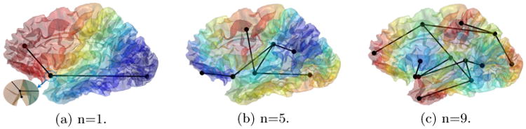
The Reeb graphs of the 1st, 5th, 9th eigenfunction of a cortical surface. In (a)-(c), the surface is color-coded with the corresponding eigenfunction. A zoomed view of a spurious critical point was shown (a).

3 Persistent Reeb Graph Matching

Based on the concept of persistence in discrete topology, we develop in this section a Reeb graph pruning and matching algorithm. This provides the core step for efficient brain search by comparing the intrinsic geometry of cortical surfaces.

For an edge $E_n^k=(C_n^i,C_n^j)$ of the Reeb Graph R(f_n) = (C_n, E_n), its weight is defined according to its persistence:

$$w(E_n^k)=|f_n(C_n^i)-f_n(C_n^j)|$$ (3)

which is the difference of the LB eigenfunction value of the two critical points $C_n^i$ and $C_n^j$. Using the weight on edges, we also have a matrix representation R_n of the Reeb graph with its entries defined as $R_n(i,j)=|f_n(C_n^i)-f_n(C_n^j)|$ if there exists an edge between the node $C_n^i$ and $C_n^j$. By using the persistence to define the edge weights, we not only have a natural way for outlier pruning but also an efficient mechanism to model the distribution of the critical points on the surface. By comparing the Reeb graphs of different surfaces, we can thus quantify their differences in terms of intrinsic geometry.

For Reeb graph pruning, an intuitive approach can be developed for the selection of a persistence threshold. Because the LB eigenfunctions have oscillatory patterns similar to Fourier basis functions, their peak values are essentially the expected persistence of the maximum and minimum. Based on this observation, we choose the persistence threshold based on the maximum of the eigenfunction as δ = max(|f_n|)/5 in our experiments. To remove spurious edges, we sort all edges according to their persistence. At each step, we find the edge $E_n^k$ with the smallest weight. If $w(E_n^k)<\delta$, we remove it from the edge set by collapsing the two nodes $C_n^i,C_n^j\in E_n^k$. For a node $C_n^i$, we calculate its total weight $S(C_n^i)$ as

$$S(C_n^i)=\sum _{C_n^i\in E_n^k}w(E_n^k).$$ (4)

We collapse the two nodes by removing the node with the smaller total weight and adding all its connections to the other node. For example, if $S(C_n^i)<S(C_n^j)$, we remove $C_n^i$ from the node set of the Reeb graph R(f_n). Except for the edge $E_n^k$ to be removed, for all other edges that were connected to $C_n^i$, we update them by replacing $C_n^i$ with $C_n^j$. We then check if the degree of any node becomes two. If so, we add an edge to connect its two neighbors and remove this node and its two edges from the graph. For all new edges, their weights are calculated according to (3) with the function values of the nodes. The above steps can be repeated until the persistence threshold is reached. For the example shown in Fig. 1, we applied the pruning process and the new results are shown in Fig. 2.

Fig. 2.

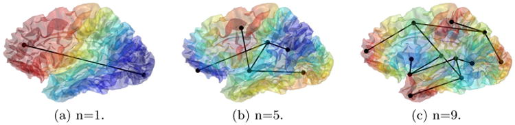
The pruned Reeb graphs.

For fast brain search, the core step is to efficiently compute a similarity measure between two cortical surfaces. The solution we develop here is based on comparing the Reeb graphs of their corresponding LB eigenfunctions. Let ℳ₁ and ℳ₂ denote two surfaces we want to compare. We denote their corresponding eigenfunctions as $f_n^1$ and $f_n^2(n=1,\dots ,N)$. For the n–th eigenfunction $f_n^1$ and $f_n^2$, we first compute their Reeb graphs $R(f_n^1)$ and $R(f_n^2)$. Let $R(f_n^1)=(C^1,E^1)$ With $C^1=(C_1^1,\dots ,C_{K_1}^1)$, $R(f_n^2)=(C^2,E^2)$ With $C^2=(C_1^2,\dots ,C_{K_2}^2)$. To start the iterative pruning and matching algorithm, we first prune both graphs to have the same number of K nodes with K ≤ min(K₁, K₂). We define the pruning cost P as the total edge weights between the original and pruned Reeb graph. The pruning cost of both graphs are denoted as $P_n^1$ and $P_n^2$. After that, an iterative process as summarized in Table 1 is applied to match the Reeb graphs of the two surfaces. Next we describe the details of each step.

Table 1. Persistent Reeb Graph Match Algorithm.

Set $D_{\mathit{min}}^n=\infty$. Repeat the following steps until the minimal edge weight of $R_n^1$ and $R_n^2$ are above the persistence threshold δ. Calculate the cost matrix D+. Calculate the cost matrix D–. Compute the distance D at the current pruning level. If $D<D_{\mathit{min}}^n$, set $D_{\mathit{min}}^n=D$ and record the correspondence. Prune the minimal edge in both Reeb graphs, and update the pruning cost $P_n^1$ and $P_n^2$. Go back to step 1.

Let K denote the number of nodes in the Reeb graphs at the start of each iteration. We define the cost matrix of size K × K for matching the nodes of $R(f_n^1)$ to $R(f_n^2)$ as

$$A^{+}(i,j)=|(S(C_i^1)-S(C_j^2)|+|f_n^1(C_i^1)-f_n^2(C_j^2)|$$ (5)

Using the cost matrix A⁺, we run the Hungarian algorithm and find the one-to-one correspondences ϕ⁺ from the nodes of $R(f_n^1)$ to $R(f_n^2)$. We compute the distance between the Reeb graphs as:

$$D^{+}=\sum _{i=1}^K\sum _{j=1}^K|R_n^1(i,j)-R_n^2({\varphi }^{+}(i),{\varphi }^{+}(j))|+\sum _{i=1}^K|f_n^1(i)-f_n^2({\varphi }^{+}(i))|$$ (6)

Where $R_n^1$ and $R_n^2$ are the matrix representation of the Reeb graphs.

Because of the sign ambiguity of the eigenfunction, we flip the sign of the eigenfunction $f_n^2$ and compute the cost matrix as

$$A^{-}(i,j)=|(S(C_i^1)-S(C_j^2)|+|f_n^1(C_i^1)+f_n^2(C_j^2)|$$ (7)

With the cost matrix A⁻, the correspondence computed with the Hungarian algorithm is denoted as ϕ⁻, and the distance between the Reeb graphs is:

$$D^{-}=\sum _{i=1}^K\sum _{j=1}^K|R_n^1(i,j)-R_n^2({\varphi }^{-}(i),{\varphi }^{-}(j))|+\sum _{i=1}^K|f_n^1(i)+f_n^2({\varphi }^{-}(i))|$$ (8)

The overall cost of the matching at the current iteration is then

$$D=min(D^{+},D^{-})+P_n^1+P_n^2$$ (9)

which is the sum of the graph distance and pruning costs. If convergence is not reached, we continue the above steps after pruning the minimal edges from both graphs as described in Table 1. Otherwise, the optimal match and the distance $D_{\mathit{min}}^n$ is recorded.

By applying the persistence Reeb graph matching algorithm for eigenfunctions up to the order N, we have the overall distance between ℳ₁ and ℳ₂ for brain search:

$$d({ℳ}_1,{ℳ}_2)=\sum _{n=1}^N{D}_{\mathit{min}}^n.$$ (10)

4 Experimental Results

In our experiments, we applied our method to T1-weighted MR images from three publicly available datasets. The first dataset consists of the 225 subjects released by the HCP up to date. The second dataset is composed of the 101 MR images of the Mindboggle atlas [12]. The third dataset includes 1000 MR images from all baseline visits of the ADNI2 project. Overall we have a total of 1326 T1-weighted images from a diverse population. Cortical surfaces were automatically reconstructed with the method in [6]. The white matter (WM) surfaces of all subjects were used in our experiments for persistent Reeb graph matching (PRGM), which is currently implemented in MATLAB. Before we perform PRGM, the first 9 LB eigenfunctions and their Reeb graphs were computed for all subjects.

4.1 Fast Brain Search

To demonstrate the capability of our method in finding the most similar brains from a large brain collection, we applied PRGM between the HCP cohorts and all brains from the three cohorts. For the left WM surface of a HCP subject, a PRGM is applied against the left WM surface of each of the 1326 subjects and the distance is computed as in (10). On a PC with a 2.7GHz CPU, every pair of PRGM takes less than 10 milliseconds. As shown in Fig. 3 (a), we obtain a distance matrix of size 225 × 1326. Among the 225 HCP subjects, the closest match for 116 of them are from the HCP collection, 15 of them are from the Mindboggle collection, and 94 of them are from the ADNI collection. As an example, we show in Fig. 3(b) the left WM surface of one HCP subject and the nearest brains we found via PRGM from all three datasets.

Fig. 3.

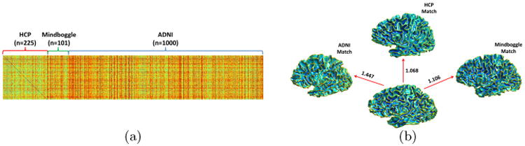
PRGM results of HCP cohorts versus the HCP, Mingboggle, and the ADNI cohorts. (a) The distance matrix. (b) The closest match of an HCP subject in the three cohorts. Distance to each matched brain is plotted alongside the arrow.

4.2 Brain Asymmetry

In our second experiment, we applied pairwise PRGM to all the left hemisphere (LH) and right hemisphere (RH) WM surfaces of the HCP cohort. The distances are saved into a matrix of size 450 × 450 as shown in Fig. 4(a), which exhibits a clear pattern: the (LH,LH) and (RH,RH) blocks of the matrix have smaller distance values than the (LH,RH) block. This suggests that we could use the PRGM distance to evaluate brain asymmetry on a large scale. To further illustrate this point, we applied multidimensional scaling (MDS) to the distance matrix and plotted the results in Fig. 4(b). While there are overlaps, it is clear that the LH and RH surfaces form very distinct clusters. A t-test was applied to the projection of the MDS embedding coordinates onto the diagonal line, i.e., the vector (−1, 1), and a highly significant p-value 9.4e−34 was obtained.

Fig. 4.

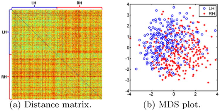
The use of persistent Reeb graph matching for brain asymmetry analysis on the HCP cohort.

4.3 Fast Resolution of Sign Ambiguity in LB embedding

To compare two surfaces with their LB embeddings as defined in (2), it is usually a challenging and computationally expensive task to resolve the ambiguities including the sign of the eigenfunctions, switching of the order of the eigenfunctions, and possible splitting of the eigenspaces due to multiplicity. With PRGM matching, we find the nearest surface from a large brain collection such that the risk of order switching is greatly reduced. For lower order eigenfunctions, multiplicity is uncommon for cortical comparisons in our experience. Thus the focus is on resolving the sign ambiguity of LB embeddings for two very similar surfaces. Using the corresponding critical points provided by PRGM, we show here that this can be achieved extremely efficiently.

For the HCP subject and its closest Mindboggle match shown in Fig. 3(b), the PRGM applied to the first 9 eigenfunctions generates a set of 48 corresponding critical points as shown in Fig. 5 (a) and (b). For the n-th eigenfunction of the first surface $f_n^1(n=1,\cdots ,9)$, we calculate its difference with $f_n^2$ or $-f_n^2$ on the corresponding point set and use the one with the smaller difference to construct the embedding of the second surface. This process can also be done in less than 10 milliseconds in our MATLAB implementation. After that, we can compute the nearest point map in the embedding space between the surfaces and pull back the manually delineated labels on the Mindboggle surface to the HCP subject [10]. The resulting labels are plotted in Fig. 5(c) and (d). For further demonstration, we plotted the cortical labeling results of six more HCP surfaces with the same strategy. These results show that excellent cortical labeling can be done efficiently with PRGM-based search. For future work, these results also lay the foundation for further improved labeling performance with the fusion of labels from multiple neighbors [10].

Fig. 5.

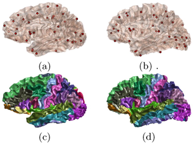
Reeb graph matching for fast sign ambiguity resolution and cortical labeling. Critical point set on the HCP (a) and Mindboggle subject (b). (c) Automatically generated labels on the HCP subject. (d) Manually delineated labels on the Mindboggle subject.

5 Conclusions

In this paper we developed a novel approach for brain search based on persistent Reeb graph matching. For future work, we will investigate different graph matching techniques and compare their speed and search performance with the Hungarian algorithm used in our current work. We will also incorporate other geometric features such as the skeletons of the sulci and gyri of the cortex for more informative comparisons.

Fig. 6.

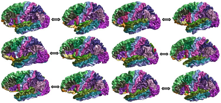
Cortical labeling results of six HCP subjects paired with their nearest match from the Mindboggle cohort. In each pair of surfaces: Left: HCP; Right: Mindboggle.

References

- 1.Mueller S, Weiner M, Thal L, Petersen RC, Jack C, Jagust W, Tro-janowski JQ, Toga AW, Beckett L. The Alzheimer's disease neuroimaging initiative. Clin North Am. 2005;15:869–877. xi–xii. doi: 10.1016/j.nic.2005.09.008. [DOI] [PMC free article] [PubMed] [Google Scholar]
- 2.Essen DV, Ugurbil K, et al. The human connectome project: A data acquisition perspective. NeuroImage. 2012;62(4):2222–2231. doi: 10.1016/j.neuroimage.2012.02.018. [DOI] [PMC free article] [PubMed] [Google Scholar]
- 3.Toga A, Clark K, Thompson P, Shattuck D, Van Horn J. Mapping the human connectome. Neurosurgery. 2012;71(1):1–5. doi: 10.1227/NEU.0b013e318258e9ff. [DOI] [PMC free article] [PubMed] [Google Scholar]
- 4.Van Horn JD, Toga A. Human neuroimaging as a “Big Data” science. Brain Imaging and Behavior. 2013:1–9. doi: 10.1007/s11682-013-9255-y. [DOI] [PMC free article] [PubMed] [Google Scholar]
- 5.Reuter M, Wolter FE, Shenton M, Niethammer M. Laplace-beltrami eigenvalues and topological features of eigenfunctions for statistical shape analysis. Computer-Aided Design. 2009;41(10):739–755. doi: 10.1016/j.cad.2009.02.007. [DOI] [PMC free article] [PubMed] [Google Scholar]
- 6.Shi Y, Lai R, Toga A. Cortical surface reconstruction via unified Reeb analysis of geometric and topological outliers in magnetic resonance images. IEEE Trans Med Imag. 2013;(3):511–530. doi: 10.1109/TMI.2012.2224879. [DOI] [PMC free article] [PubMed] [Google Scholar]
- 7.Edelsbrunner, Letscher, Zomorodian Topological persistence and simplification. Discrete Comput Geom. 2002;28(4):511–533. [Google Scholar]
- 8.Lee H, Kang H, Chung M, Kim BN, Lee DS. Persistent brain network homology from the perspective of dendrogram. IEEE Trans Med Imag. 2012;31(12):2267–2277. doi: 10.1109/TMI.2012.2219590. [DOI] [PubMed] [Google Scholar]
- 9.Rustamov RM. Laplace-beltrami eigenfunctions for deformation invariant shape representation. Proc Eurograph Symp on Geo Process. 2007:225–233. [Google Scholar]
- 10.Shi Y, Lai R, Toga AW. Conformal mapping via metric optimization with application for cortical label fusion. Proc IPMI. 2013:244–255. doi: 10.1007/978-3-642-38868-2_21. [DOI] [PMC free article] [PubMed] [Google Scholar]
- 11.Reeb G. Sur les points singuliers d'une forme de Pfaff completement integrable ou d'une fonction nemèrique. Comptes Rendus Acad Sciences. 1946;222:847–849. [Google Scholar]
- 12.Klein A, Tourville J. 101 labeled brain images and a consistent human cortical labeling protocol. Frontiers in Neuroscience. 2012;6(171) doi: 10.3389/fnins.2012.00171. [DOI] [PMC free article] [PubMed] [Google Scholar]