Biochemistry and Theory of Proton-Coupled Electron Transfer

1. Introduction and Motivation

Through incremental change, Nature reworks and repurposes its functional machinery. In this way, proteins that photochemically repair DNA by moving protons and electrons have a structural and functional link to proteins that are implicated in bird navigation.¹ A protein that reduces NO but pumps no protons is similar to a protein that reduces O₂ and pumps protons.^2,3 Biology employs reactions with intricate coupling of proton and electron movement, so-called proton-coupled electron transfer (PCET). Biological PCET underpins photosynthesis and respiration, light-driven cell signaling, DNA biosynthesis, and nitrogen fixation in the biosphere.⁴ The scope of natural PCET reactions is as breathtaking as the possible quantum chemical mechanisms that underlie them. Considerable focus has been placed on uncovering how specific proteins utilize PCET in their function. Cytochrome c oxidase oxidizes cytochrome c and reduces and protonates O₂ to water.² Sulfite reductase reduces SO₃^2– to S^2– and water with the help of protons.⁵ BLUF domains switch from light to dark states via oxidation and deprotonation of a tyrosine.⁶ Are there overarching mechanistic themes for these seemingly disparate PCET reactions? For instance, do certain protein amino acids promote different biological PCET reactions? Is the dielectric environment important? How do the (quantum and classical) laws of motion and the statistical mechanics of complex assemblies constrain the structure and function of PCET assemblies? Knowledge of individual PCET protein structure and function, combined with a predictive theoretical framework, encourage us to seek general principles that may guide both protein design and understanding of biological PCET. To better inform protein design, we must look very closely at examples of biological PCET mechanisms and at the underpinnings of the theoretical foundations governing these critical reactions.

Since electrons and protons have very different masses, they can tunnel over very different distances. Thus, not surprisingly, in many PCET reaction mechanisms, the electron donor–acceptor pair differs from the proton donor–acceptor pair (for example, long-distance electron transfer (ET) coupled to proton transfer (PT) at a hydrogen-bonded interface inspired Cukier’s theory; see sections 2.1.1 and 11). In other circumstances (see sections 5, 7, and 12), the electron and proton transfer between the same chemical donor and acceptor, as occurs for hydrogen atom transfer. This diversity contributes to the richness of PCET reaction mechanisms.

The relative time scales of ET and PT reactions depend dramatically on the respective transfer distances, as well as on the environmental (nuclear) motions that couple to the two reactions. Therefore, the time scales of the reactive electron and proton motions also need to be compared with relevant time scales of the environment (e.g., solvent and/or protein). Nature has evolved a diverse array of PCET reactions, ranging from distinctly sequential electron and proton transfer reactions (where the first reaction precedes and promotes the second one, so that the two events are coupled although temporally separated; for example, see section 8) to simultaneous or concerted transfer, with a wide range of intermediate regimes whose difficult interpretation has prompted the development of several experimental and theoretical methods (e.g., see sections 7, 11, and 12).

Fluctuations of PCET systems are particularly significant (e.g., see sections 10 and 12), because structural changes can dramatically change the time scales of motion required for the reaction. Addressing such fluctuations defines a current rich frontier for theory and experiment.

Electron and proton sources and sinks, time scales of motion, energetics, and structural fluctuations have been the objects of evolutionary forces. These terms appear prominently in the theory, described by free energy parameters (e.g., reaction free energy and reorganization energy) and electronic and vibronic couplings. At the atomistic level, critical questions remain as to dominant pathways, or families of pathways, for proton and electron motion from their initial to their final positions (or ensembles of positions). Indeed, given the exponential sensitivity of rates to reaction barriers, the fluctuations of these pathways and of their energetics is a focal point of intense current interest (e.g., see sections 5, 10, and 12). Biological cofactors and amino acids can play active roles in PCET pathways, and understanding the ET and PT pathways (e.g., see section 8) sheds light on reaction and control mechanisms. Ultimately, PCET is influenced by the topology and geometry of thermally fluctuating interacting components in chemical and biological systems. The topological and geometric factors that control PCET reactions are a central theme in the experimental and theoretical analysis of this review.

This review has the following structure: (i) The amino acid radical environments of tryptophan and tyrosine are elaborated for a handful of proteins that utilize these amino acids for PCET. Part i provides primarily experimental results, although some theoretical work is also discussed. (Indeed, theory is often essential to elucidate mechanism for PCET in these and related systems.) This part also emphasizes the possible complications in PCET mechanism (e.g., sequential vs concerted charge transfer under varying conditions) and sets the stage for part ii of this review. (ii) The prevailing theories of PCET, as well as many of their derivations, are expounded and assessed. This is, to our knowledge, the first review that aims to provide an overarching comparison and unification of the various PCET theories currently in use.

While PCET occurs in biology via many different electron and proton donors, as well as involves many different substrates (see examples above), we have chosen to focus on tryptophan and tyrosine radicals as exemplars due to their relative simplicity (no multielectron/proton chemistry, such as in quinones), ubiquity (they are found in proteins with disparate functions), and close partnership with inorganic cofactors such as Fe (in ribonucleotide reductase), Cu, Mn, etc. We have chosen this organization for a few reasons: to highlight the rich PCET landscape within proteins containing these radicals, to emphasize that proteins are not just passive scaffolds that organize metallic charge transfer cofactors, and to suggest parts of PCET theory that might be the most relevant to these systems. Where appropriate, we point the reader from the experimental results of these biochemical systems to relevant entry points in the theory of part ii of this review.

1.1. PCET and Amino Acid Radicals

Proteins organize redox-active cofactors, most commonly metals or organometallic molecules, in space. Nature controls the rates of charge transfer by tuning (at least) protein–protein association, electronic coupling, and activation free energies.^7,8 In addition to bound cofactors, amino acids (AAs) have been shown to play an active role in PCET.⁹ In some cases, such as tyrosine Z (TyrZ) of photosystem II, amino acid radicals fill the redox potential gap in multistep charge hopping reactions involving several cofactors. The aromatic AAs, such as tryptophan (Trp) and tyrosine (Tyr), are among the best-known radical formers. Other more easily oxidizable AAs, such as cysteine, methionine, and glycine, are also utilized in PCET. AA oxidations often come at a price: management of the coupled-proton movement. For instance, the pK_a of Tyr changes from +10 to −2 upon oxidation and that of Trp from 17 to about 4.¹⁰ Because the Tyr radical cation is such a strong acid, Tyr oxidation is especially sensitive to H-bonding environments. Indeed, in two photolyase homologues, H-bonding appears to be even more important than the ET donor–acceptor (D–A) distance.¹¹ Discussion concerning the time scales of Tyr oxidation and deprotonation indicates that the nature of Tyr PCET is strongly influenced by the local dielectric and H-bonding environment. PCET of TyrZ is concerted at low pH in Mn-depleted photosystem II, but is proposed to occur via PT and then ET at high pH (vide infra).¹² In either case, ET before PT is too thermodynamically costly to be viable. Conversely, in the Slr1694 BLUF domain from Synechocystis sp. PCC 6803, Tyr oxidation precedes or is concerted with deprotonation, depending on the protein’s initial light or dark state.¹³ In general, Trp radicals can exist either as protonated radical cations or as deprotonated neutral radicals. Examples of both forms are found in DNA photolyase.^1,14 The management of protons coupled to AA oxidations may provide a means for a protein to control the timing of chemical reactions via protein structural changes and fluctuations. In general, proton transfer requires the proximity of the proton donor and acceptor to be within the distance of a typical H-bond (∼2.8 Å between heavy atoms). Any protein dynamics that shifts this H-bond distance can thus considerably influence the reaction kinetics.

An argument can be posited that almost all charge transfer in biology is proton-coupled on some time scale to prevent the buildup of charge in the low dielectric environment characteristic of proteins. However, proteins are anisotropic and have atomic-scale structure, so the utility of a dielectric constant itself may be questioned, and estimated dielectric parameters may vary on the length scale of a few AAs. What is the nature of the protein environment surrounding AA radicals in different proteins? What do these proteins have in common, if anything? Below, we compare the Tyr and Trp environments of proteins that utilize these AA radicals in their function. (For a more detailed view of the local protein environments surrounding these Tyr and Trp radicals, see Figures S1–S9 of the Supporting Information.) This side-by-side comparison may begin to suggest design principles associated with AA radical PCET proteins. To better inform protein design, we must look more closely at PCET in these proteins and, finally, appreciate the underlying physical mechanisms and physical constraints at work.

1.2. Nature of the Hydrogen Bond

Because hydrogen bonding is critical for proton and proton-coupled electron transfer, we now explore the criteria that give rise to strong or weak hydrogen bonds. Since hydrogen atoms are rarely resolved in electron density maps, a hydrogen bond (H-bond) distance is traditionally characterized by the distance between donor and acceptor heteroatoms (R_O···O, R_N···O, R_N···N, etc.).¹⁵ Normal H-bond distances between oxygen heteroatoms are 2.8–3.0 Å.^15,16 In fact, a hydrogen bond is often posited when R_A···B < R_A + R_B, where R_A and R_B are the van der Waals radii of two heteroatoms and R_A···B is the distance between heteroatom nuclei. Strong hydrogen bonds are defined as R_A···B ≪ R_A + R_B, typically <2.6 Å for R_O···O, and tend to be ionic in nature.¹⁵ Here, ionic refers to a positively charged H-bond donor and/or a negatively charged H-bond acceptor, i.e., A⁺–H···B^—. (A negatively charged H-bond acceptor is more strongly attracted to the partial positive charge of the H-bond donor, and similarly, a positively charged donor is more strongly attracted to the partial negative charge of the H-bond acceptor. An example of such an ionic bond would be N⁺–H···O^— of a doubly protonated histidine and a deprotonated tyrosinate anion.) Even if R_A···B ≥ R_A + R_B, weak H-bonds are defined as R_H···B < R_H + R_B, where R_H is the van der Waals radius of hydrogen and R_H···B is the radial distance between the donor hydrogen and the acceptor heteroatom centers. Because H-bonds, especially weak ones, can be easily deformed in crystal lattices, the H-bond angle tends to be a less reliable discriminator of strong vs weak bonds. (If a H-bond is dominated by electrostatic interactions, the heteroatom-H-heteroatom bond angle will be nonlinear, given the roles of heteroatom lone pair orbitals in the donor−acceptor interaction.)

There is some debate concerning the existence of “low-barrier” vs “short, strong, ionic” H-bonds, particularly in the field of serine protease enzymology,^17,18 but also within the area of natural photosynthesis.^19,20 TyrZ of photosystem II (vide infra) has a particularly short hydrogen bond (2.5 Å) with a nearby histidine.²¹ A typical H-bond energy viewed against the proton position would trace a standard double-well potential (Figure 1, left), with the difference in pK_a of the H-bond donor and acceptor giving rise to the energy difference between minima of the two wells. Low-barrier H-bonds (LBHBs) have a reduced barrier between the wells due to the shorter distance between the H-bond donor (A–H) and acceptor (B), with barrier heights approximately equal to or below the proton vibrational energy (Figure 1, center).²² The deuterium vibrational energy may be lower than the barrier, leading to significant isotope effects, such as a reduction in the ratio of IR stretching mode frequencies between H and D (ν_H/ν_D) and a fractionation factor of ∼0.3.^16,23 (The fractionation factor is the ratio of deuterium to hydrogen within the H-bond due to equilibrium isotope exchange with water.) The most distinguishing characteristic of a low-barrier H-bond is a similar distance of the shared proton from the donor and the acceptor (see Figure 1, center). In the case of a barrierless, single-well potential, the proton would be shared equally between the H-bond donor and acceptor (Figure 1, right). Matching of the H-bond donor and acceptor pK_a as well as shortening the H-bond distance leads to a flatter well potential and stronger H-bond, since the two protonated states would have nearly equal energies and strong coupling.²³

Figure 1.

Zero-point energy effects in (left) weak, (center) strong, and (right) very strong hydrogen bonds. The hydrogen vibrational level (H) is depicted above the barrier for a strong H-bond. The deuterium vibrational level (D) is depicted below the barrier for weak and strong H-bonds, whereas the barrier is absent for very strong H-bonds. The proton is attached to the H-bond donor (A–H), and the H-bond acceptor is B. The reaction coordinate is the A···H bond distance, shown for different distances between A and B.

Although formation of LBHBs in biology remains controversial,^24,25 clearly H-bond formation is key in PCET processes. One example involves a hypothesized model of PCET in TyrZ of photosystem II, where TyrZ forms an LBHB with histidine 190 of the D1 protein, which becomes a weak H-bond upon TyrZ oxidation and proton transfer.²⁰ Although still speculative, some experiments and quantum chemical calculations suggest that TyrD of photosystem II (vide infra) in its singlet ground state forms a normal H-bond to histidine 189 of the D2 protein, whereas at pH > 7.6, TyrD and histidine 189 form a short, strong H-bond.^26,27 Tyr122 of ribonucleotide reductase has also been shown to switch H-bonding states upon oxidation, where the Tyr neutral radical moves away from its previously established H-bonded network.²⁸

One of the most important chemical consequences of H-bonds is that they often act as a conduit for proton transfer (although in rare cases, proton transfer may occur without the formation of a H-bond).^29,30 Indeed, the same factors leading to strong H-bonds can also lead to efficient PT. Through manipulation of the amino acid (and bound cofactor) pK_a—for instance, via direct H-bonds or electron transfer events—proteins can modulate the driving force for PT.³¹ In this way, we see that H-bond formation is strongly tied to PCET in chemistry and biology. The equilibrium positions of the proton before and after PT are important in the underlying PT kinetics (e.g., see section 10); however, knowledge of the geometry and energetics of the transition-state complex is critical for a correct interpretation of and insight into the PCET mechanism (see sections 5 and 7–12). In this regard, theoretical investigations of PCET reactions have proven invaluable.^32,33

2. Tyrosyl Radical Environments

Tyr is a major player in many important PCET proteins, such as photosystem II,³⁴ ribonucleotide reducatase,^35,36 galactose oxidase,³⁷ cyctochrome c oxidase,² and many more. The proton-coupled nature of Tyr oxidation is often relevant and integral in biochemical reactions as diverse as water oxidation and ribonucleotide reduction. The Tyr redox potential is highly sensitive to pH and therefore the presence or absence of nearby bases to which Tyr could form a H-bond. For example, Tyr-OH oxidation to Tyr-OH^•+ at pH < 2 has a midpoint potential greater than 1.2 V vs. NHE, whereas, at a pH of 7, the Tyr midpoint potential is 0.9 V.¹⁰ This means the oxidizing power of the Tyr radical varies with its protonation state. Tyr has been demonstrated to perform both reductive and oxidative roles in relation to inorganic metal cofactors bound in proteins. For instance, the neutral radical Tyr-O^• (TyrZ) is capable of oxidizing the manganese–calcium water-oxidizing complex in photosystem II, whereas Tyr-OH reduces a diiron complex in class Ia ribonucleotide reductase at the beginning of a long-distance radical transfer chain.^36,38 In the following section, we explore the roles of Tyr in several proteins and their relation to inorganic cofactors. The PCET reactions involved with Tyr can display quite different character. Where appropriate connections can be made between these experimental results and theory, we point the reader to relevant theoretical sections of this review.

2.1. Photosystem II

Photosystem II (PSII) of green plants and cyanobacteria is a multiprotein, membrane-associated complex that converts, transduces, and stores photonic energy in the form of chemical potential energy, initially as a proton gradient and ultimately as new chemical bonds.^34,39−42 PSII uses water as a reductant of photo-oxidized chlorophyll and after four such reductions produces molecular oxygen.

PSII is often invoked as a paradigm of biological PCET (see Figure 2), with proton-coupled redox processes occurring during tyrosine oxidation and reduction, water oxidation, and quinone reduction.^43,44 The remarkable quantum efficiency of PSII has encouraged many researchers to develop synthetic models to mimic its PCET reactions. These models initially focused on photoinduced electron transfer in covalently linked donor–bridge–acceptor (D–Br–A) quinone systems.⁴⁵⁻⁴⁸ Models for Tyr radical formation have also been developed and coupled to a Mn cluster similar to the water-oxidizing complex (WOC).^{39−42,49,50}

Figure 2.

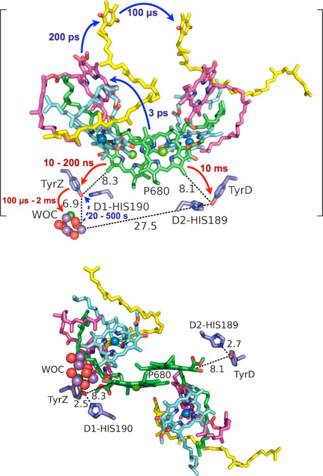
Top: Time scales of electron transfer (blue arrows) and hole transfer (red arrows) of the initial photosynthetic charge transfer events in PSII, including water oxidation.⁵¹⁻⁵³ The time scale of unproductive back electron transfer from the WOC to TyrZ is shown with a dashed arrow. Auxiliary chlorophylls are shown in light blue, pheophytins in magenta, and quinones A (Q_A) and B (Q_B) in yellow. WOC = water-oxidizing complex. Distances shown (dotted lines) are in angstroms. The brackets emphasize that the protein complex is housed within a bilayer membrane. Bottom: Alternative view of the PSII reaction center displaying the locations of TyrZ and TyrD in relation to P680, with H-bond distances to histidine (His) shown in angstroms. The figure was rendered using PyMol.⁵⁴

To separate an electron and hole over 25 Å across a membrane, PSII utilizes multistep charge hopping on many different time scales (Figure 2). Control over these time scales is intimately linked to the nearby protein environment of each cofactor. The reaction center (RC) of PSII is housed in the D1 and D2 proteins (chains a and d of PDB 3ARC) and consists of two diverging and symmetric branches of cofactors that share a special pair of chlorophylls (P680). Each branch has an auxiliary chlorophyll, a pheophytin, and a quinone. As only one branch of the RC is active (see Figure 2 for the directionality of ET), these branches have functionally important asymmetries.⁵⁵ Notably, each branch has an associated tyrosine–histidine pair that produces a tyrosyl radical, but each radical displays different kinetic and thermodynamic behavior. Tyr 161 (TyrZ) of the D1 protein, nearest the WOC, is required for PSII function, as discussed in the next section, while Tyr 160 (TyrD) of the D2 protein is not essential and may correspond to a vestigial remnant from an evolutionary predecessor that housed two WOCs.³⁸ These Tyr radicals serve as excellent models for Tyr oxidations in proteins due to their symmetrically similar environments yet drastic differences in kinetics and thermodynamics. Their important role in the process of oxygen-evolving photosynthesis (and consequently all life on earth) has led these radicals to become among the most studied Tyr radicals in biology.

2.1.1. D1-Tyrosine 161 (TyrZ)

Tyrosine 161 (TyrZ) of the D1 protein subunit of PSII acts as a hole mediator between the WOC and the photo-oxidized P680 chlorophyll dimer (P680^•+) (see Figure 2). Its presence is obligatory for oxygen evolution, along with its strongly H-bonded partner histidine 190 (His190).⁴⁴ Photosynthetic function cannot be recovered even by TyrZ mutation to Trp, one of the most easily oxidized AAs.⁵⁶ This might be rationalized by aqueous redox measurements of these AAs between pH > 3 and pH < 12, which point to Tyr being slightly easier to oxidize than Trp in this range.¹⁰ However, these measurements at pH < 3 make apparent that protonated Tyr-OH is more difficult to oxidize than protonated Trp-H, such that management of the phenolic proton is often a requirement for Tyr oxidation in proteins. (Mutation of His190 to alanine also impairs the electron donor function of TyrZ, which can be recovered by titration of imidazole.⁵⁷). TyrZ is a H-bond donor to His190, which is in turn a H-bond donor to asparagine 298 (see Figure 3). The H-bond length R_O···N is unusually short (2.5 Å), indicating a very strong H-bond.

Figure 3.

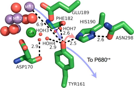
Model of the protein environment surrounding Tyr161 (TyrZ) of photosystem II from T vulcanus (PDB 3ARC). Distances shown (dashed lines) are in angstroms. Crystallographic waters (HOH = water) are shown as small, red spheres and the WOC as large spheres with Mn colored purple, oxygen red, and Ca green. The directions of ET and PT are denoted by transparent blue and red arrows, respectively. The figure was rendered using PyMol.⁵⁴

Under physiological conditions (pH ≈ 6.5 or less) oxidation of TyrZ by P680^•+ appears to be concerted with deprotonation to His190 to form the H-bonded pair TyrZ-O^•···HN⁺-His190.¹² The transferred proton may then rock back to TyrZ-O^• upon reduction of TyrZ by the WOC, or it may exit to the lumen through a H-bonded pathway of amino acids and waters.^31,58 Both fates for the phenolic proton have been suggested in the literature, and perhaps both are possible depending on which part of the Kok cycle the WOC is in. (The Kok cycle is the five states, S₀ through S₄, that characterize the oxidation states of the WOC during the proton-coupled oxidation of water to molecular oxygen. The current view of proton release during transitions between these states is one (S₀ → S₁), zero (S₁ → S₂), one (S₂ → S₃), and two (S₃ → S₄) protons.⁵⁸) If the phenolic proton remains on HN⁺-His190, the positive charge of the doubly protonated imidazole may drive shifts in the pK_a values of nearby protonatable residues and thus act as a gating mechanism for proton transduction from the WOC to the bulk.⁵⁸

TyrZ oxidation—which is often probed by monitoring the recovery of P680 from P680^•+—is multiphasic, with a fast time component of ∼10 ns and a longest time component of ∼0.5 μs.¹² A hypothesis has been proposed that the fastest component of TyrZ oxidation displayed by O₂-evolving PSII is characteristic of oxidation of an equilibrated population of TyrZ-O^•– ···HN⁺-His190. Indeed, QM calculations have shown that the H-bond distance of this ion pair is equivalent (2.46 Å) to that in the neutral pair (TyrZ-OH···N-His190).¹⁹ The slower components of Tyr oxidation may involve slower protein motions that promote proton transfer or protein relaxation.¹² The redox potential of TyrZ has been estimated to lie around 1 V vs NHE and to have a pK_a of 10.3–12, while His190 has a pK_a = 7–7.5 in Mn-depleted PSII.³⁸ The presence of the WOC seems to provide a sufficiently strong electrostatic influence to lower the pK_a of His190 by 2–3 log units (pK_a ≈ 4–5) in O₂-evolving PSII. Because the “working pH” for O₂-evolving PSII is ∼5.5–7, His190 should be neutral, allowing it to act as a H-bond acceptor of the phenolic proton of TyrZ.³⁸

The WOC reduces TyZ-O^• in the microsecond to millisecond time regime. For a longer lived radical signal, the WOC is removed by treatment with detergent in so-called Mn-depleted PSII preparations. In Mn-depleted PSII, the H-bonding environment around TyrZ could be drastically modified, leading to changes in the kinetics and even the PCET mechanism. For instance, the X-ray crystal structure of PSII from Thermosynechococcus vulcanus (PDB 3ARC) shows Ca²⁺ organizes two water molecules that H-bond with TyrZ.²¹ These water molecules are part of a group of four water molecules that may play a large role in shortening the TyrZ-OH···N-His190 H-bond distance, which would reduce the energy barrier for proton transfer.¹⁹ Indeed, in Mn-depleted PSII, the radical signal of TyrZ-O^• is not observed at liquid helium temperatures, nor is it observed at high pH (>7.6) in photosynthetically competent PSII.⁵⁹ This implies the presence of an energetic barrier to proton transfer from TyrZ-OH to His190 at high pH and in Mn-depleted PSII preparations (see Figure 1, left, in section 1.2 and Figure 21a in section 5.3.1). Therefore, at high pH (>7.6), sequential PT and then ET may play a larger role in TyrZ redox behavior. The TyrZ-O^• radical signal is present however at low pH (<6.5), indicating that under physiological conditions TyrZ experiences a barrierless potential to proton transfer and a strong H-bond to His190 (see Figures 1, right, in section 1.2 and 21b in section 5.3.1).^19,31,60

Figure 21.

Schematic depiction of the effective potential energies for the proton motion and associated vibrational levels in (a) electronically adiabatic and vibrationally nonadiabatic or (b) electronically and vibrationally adiabatic PT (coupled to ET in the PCET context). A surface with a single minimum is formed at very short proton donor–acceptor distances (such as X ≲ 2.5 Å). For example, TyrZ in PSII has a very strong hydrogen bond with His190, with a bond length at the upper bound of the range considered here. A single minimum may arise for extremely strongly interacting molecules, with very short hydrogen bonds.²¹⁹

The protein seems to play an integral role in the concerted oxidation and deprotonation of TyrZ, in the sense that protein backbone and side chain interactions orient water molecules to polarize their H-bonds in particular ways. The backbone carbonyl groups of D1-pheylalanine 182 and D1-aspartate 170 orient two key waters in a diamond cluster that H-bonds with TyrZ, which may modulate the pK_a of TyrZ (see Figure 3). The WOC cluster itself seems responsible for orienting particular waters to act as H-bond donors to TyrZ, with Ca²⁺ orienting a key water (W3 in ref (26), HOH3 in Figure 3).

The local polar environment around TyrZ is mostly localized near the WOC, with amino acids such as Glu189 and the five-water cluster. Away from the WOC, TyrZ is surrounded by hydrophobic amino acids, such as phenylalanine (182 and 186) and isoleucine (160 and 290) (see Figure S1 in the Supporting Information). These hydrophobic amino acids might shield TyrZ from “unproductive” proton transfers with water, or may steer water toward the WOC for redox chemistry. A combination of the hydrophobic and polar side chains seems to impart TyrZ with its unique properties and functionality.

TyrZ so far contributes the following knowledge regarding PCET in proteins: (i) short, strong H-bonds facilitate concerted electron and proton transfer, even among different acceptors (P680^•+ for ET and D1-His190 for PT); (ii) the protein provides a special environment for facilitating the formation of short, strong H-bonds; (iii) the pH of the surrounding environment—i.e., protonation state of nearby residues—may change the mechanism of PCET (e.g., from concerted to sequential; for synthetic analogues, see, for instance, the work of Hammarström et al.^50,61).

2.1.2. D2-Tyrosine 160 (TyrD)

D2-Tyr160 (TyrD) of PSII and its H-bonding partner D2-His189 form the symmetrical counterpart to TyrZ and D1-His190. However, the TyrD kinetics is much slower than that of TyrZ. The distance from P680 is practically the same (∼8 Å edge-to-edge distance from the phenolic oxygen of Tyr to the nearest ring group, a methyl, of P680; see Table 1), but the kinetics of oxidation is on the scale of milliseconds for TyrD, and its kinetics of reduction (from charge recombination) is on the scale of hours. TyrD, with an oxidation potential of ∼0.7 V vs NHE, is easier to oxidize than TyrZ, so its comparatively slow PCET kinetics must be intimately tied to management of its phenolic proton. Interestingly, TyrD PCET kinetics is only slow at physiological pH. At pH > 7.7, the rate of oxidation of TyrD approaches that of TyrZ.⁶² At pH > 7.7, oxidations of TyrZ and TyrD by P680^•+ in Mn-depleted PSII are as fast as 200 ns.⁶² However, below pH 7.7, TyrD oxidation occurs in the hundreds of microseconds to milliseconds regime, which differs drastically from the kinetics of TyrZ oxidation. For example, at pH 6.5, TyrZ oxidation occurs in 2–10 μs, whereas that of TyrD occurs in >150 μs.⁶²

Table 1. Amino Acid Radical Properties Found in Various Proteins.

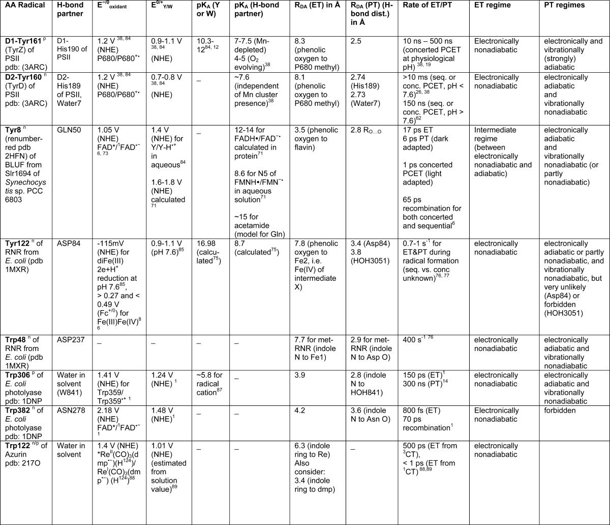
ⁿAA is in a non-polar protein environment.

^PAA is in a polar protein environment.

TyrD-O^• forms under physiological conditions via equilibration of TyrZ-O^• with P680^•+ in the S₂ and S₃ stages of the Kok cycle.⁶⁰ The equilibrated population of P680^•+ allows for the slow oxidation of TyrD-OH, which acts as a thermodynamic sink due to its lower redox potential. Whereas oxidized TyrZ-O^• is reduced by the WOC at each step of the Kok cycle, TyrD-O^• is reduced by the WOC in S₀ of the Kok cycle with much slower kinetics, so that most “dark-adapted” forms of PSII are in the S₁ state.⁶⁰ TyrD-O^• may also be reduced through the slow, long-distance charge recombination process with quinone A^•–. If indeed the phenolic proton of TyrD associates with His189, creating a positive charge (H⁺N-His189), the location of the hole on P680^•+ may be pushed toward TyrZ, accelerating oxidation of TyrZ. Recently, high-frequency electronic–nuclear double resonance (ENDOR) spectroscopic experiments indicated a short, strong H-bond between TyrD and His189 prior to charge transfer and elongation of this H-bond after charge transfer (ET and PT). On the basis of numerical simulations of high-frequency ²H ENDOR data, TyrD-O^• is proposed to form a short 1.49 Å H-bond with His189 at a pH of 8.7 and a temperature of 7 K.²⁷ (Here, the distance is from H to N of His189.) This H-bond is indicative of an unrelaxed radical. At a pH of 8.7 and a temperature of 240 K, TyrD-O^• is proposed to form a longer 1.75 Å H-bond with His189. This H-bond distance is indicative of a thermally relaxed radical. Because the recent 3ARC (PDB) crystal structure of PSII was likely in the dark state, TyrD was most likely present in its neutral radical form TyrD-O^•. The heteroatom distance between TyrD-O^• and N-His189 is 2.7 Å in this structure, which could represent the “relaxed” structure, i.e., the equilibrium heteroatom distance for this radical. At least at high pH, these experiments corroborate that TyrD-OH forms a strong H-bond with His189, so that its PT to His189 may be barrierless. On the basis of these ENDOR data for TyrD, PT may occur before ET, or perhaps a concerted PCET mechanism is at play. Indeed, at cryogenic temperatures at high pH, TyrD-O^• is formed whereas TyrZ-O^• is not.⁶⁰ Many PCET theories are able to describe this change in equilibrium bond length upon charge transfer. For an introduction to the Borges–Hynes model where this change in bond length is explicitly discussed and treated, see section 10.

Why is TyrD easier to oxidize than TyrZ? Within a 5 Å radius of the TyrD side chain lie 12 nonpolar AAs (green shading in Table 2) and 4 polar residues, which include the nearby crystallographic “proximal” and “distal” waters. This hydrophobic environment is in stark contrast to that of TyrZ in D1, which occupies a relatively polar space. For TyrD, phenylalanines occupy the corresponding space of the WOC (and the ligating Glu and Asp) within the D1 protein, creating a hydrophobic, (nearly) water-tight environment around TyrD. One might expect a destabilization of a positively charged radical state in such a comparatively hydrophobic environment, yet TyrD is easier to oxidize than TyrZ by ∼300 mV. The positive charge due to the WOC, as well as H-bond donations from waters (expected to raise the redox potentials by ∼60 mV each³¹) might drive the TyrZ redox potential more positive relative to TyrD.

Table 2. Local Protein Environments Surrounding Amino Acid Tyr or Trp That Are Redox Active^a.

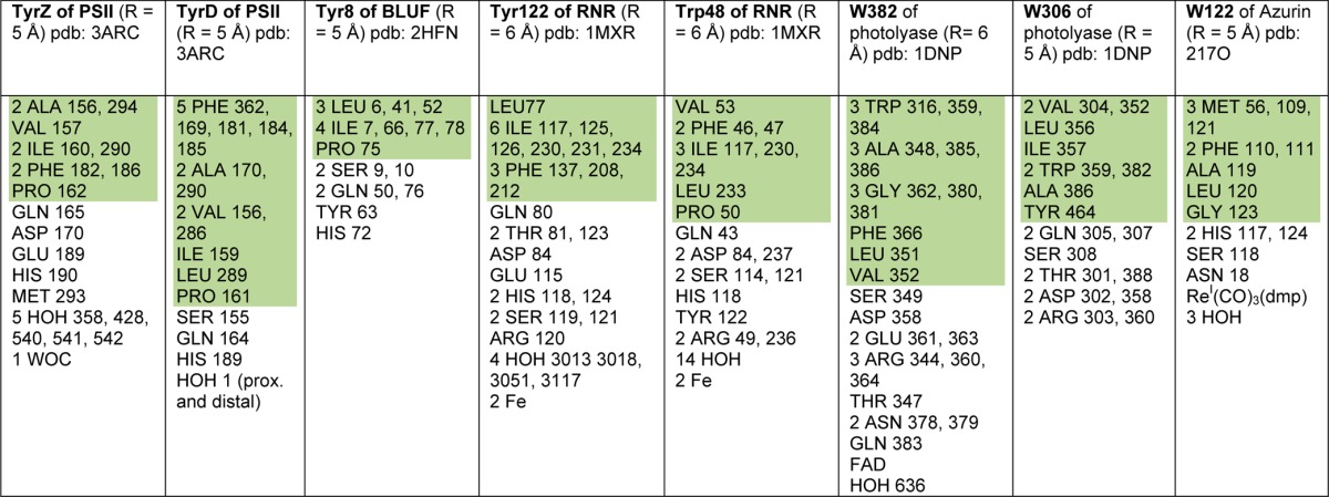
^aHydrophobic residues are shaded green, and polar residues are not shaded.

The fate of the proton from TyrD-OH is still unresolved. Indeed, the proton transfer path may change under various conditions. Recently, a proximal water, as opposed to His189, was suggested as the phenolic proton acceptor during PCET from TyrD-OH under physiological conditions (pH < 6.5).^26,63 High-field ²H Mims-ENDOR spectroscopic studies of the TyrD-O^• radical at a pD (deuterated sample) of 7.4 from WOC-present PSII indicate His189 as the only H-bonding partner to TyrD-O^•.⁶⁴ However, this does not preclude TyrD-OH from H-bonding to a proximal water which then translocates upon acceptance of the phenolic proton. Indeed, at pH 7.5, FTIR evidence (changes in the His189 stretching frequency) points to His189 as a proton donor to TyrD-O^• in Mn-depleted PSII.⁶⁵ However, FTIR spectra also indicate that two water molecules reside near TyrD in Mn-depleted PSII at pH 6.0.⁶³ Of these two waters, one is strongly H-bonded and the other weakly H-bonded; these water molecules change H-bond strength upon oxidation of TyrD. The recent crystal structure of PSII (PDB 3ARC) with 1.9 Å resolution shows the electron density for occupancy of a single water molecule at two distances near TyrD. The proximal water is 2.7 Å from the phenolic oxygen of TyrD, whereas the so-called distal water is out of H-bonding distance at 4.3 Å from the phenolic oxygen. Recent QM calculations associate the proximal water configuration with the reduced, protonated TyrD-OH and the distal water configuration as the most stable for the oxidized, deprotonated TyrD-O^•.²⁶ Since TyrD is likely predominantly in its radical state TyrD-O^• during crystallographic measurements, the distal water should show a greater propensity of occupancy in the solved structure. Indeed, this is the case (65% distal vs 35% proximal). An even more recently solved structure of PSII from T. vulcanus with 2.1 Å resolution and Sr substitution for Ca shows no occupancy of the proximal water (both structures were solved at pH ≈ 6.5).⁶⁶ Notably, no H-bond donor fills the H-bonding role of the proximal water to TyrD in this structure, yet all other H-bonding distances are the same. Due to this suggested evidence of water as a proton acceptor to TyrD-OH under physiological conditions and His189 as a proton acceptor under conditions of high pH, we must take a closer look at the protein environment which may enable this switching behavior.

Although D1-His190 and D2-His189 share the identity of one H-bond partner (Tyr), their second H-bonding partners differ. D1-His190 is H-bonded to the carbonyl oxygen of asparagine 298, whereas D2-His189 is H-bonded to arginine 294 (see Figures 3 and 4). At physiological pH, the H-bonded nitrogen of the guanidinium group of arginine 294 is protonated (the pK_a of arginine is ∼12), which forces arginine 294 to act as a H-bond donor to D2-His189. On the contrary, asparagine 298 acts as a H-bond acceptor to D1-His190. This should have profound implications for the fate of the phenolic proton of TyrD vs TyrZ, since the proton-accepting ability of His189/190 from TyrD/Z is affected. At physiological pH, D2-His189 is presumably forced to act as a H-bond donor to TyrD-OH. At high pH, if arginine 294 or His189 becomes deprotonated (doubly deprotonated in the case of His189), the capability of His189 to act as a proton acceptor from TyrD is restored. This may explain the barrierless PT from TyrD-OH to (presumably) His189 at pH > 7.6. Although water is not an energetically favored proton acceptor (its pK_a is 14), Saveant et al. found that water in water is an intrinsically favorable proton acceptor of a phenolic proton as compared to bases such as PO₄H₂^–.⁶⁷ A reason for this includes a smaller reorganization energy when the proton can be delocalized over several water molecules in a Grotthus-type mechanism. Indeed, Saito et al. describe that movement of the proximal water (now a positively charged hydronium ion) 2 Å to the distal site, where the proton may concertedly transfer via several H-bonded residues and waters to the bulk, as a possible mechanism for the prolonged lifetime of the TyrD-O^• radical. It is tempting to suggest, that under physiological pH, TyrD-OH forms a normal H-bond with a proximal water, which may result in slow charge transfer kinetics due to the large difference in pK_a as well as a larger barrier for PT, whereas, at high pH, the now-allowed PT to His189 leads to PT through a strong H-bond with a more favorable change in pK_a. (See section 10 for a discussion concerning the PT distance and its relationship to PT coupling and splitting energies.) Although the proton path from TyrD is not settled, the possibility of water as a proton acceptor still cannot be excluded.

Figure 4.

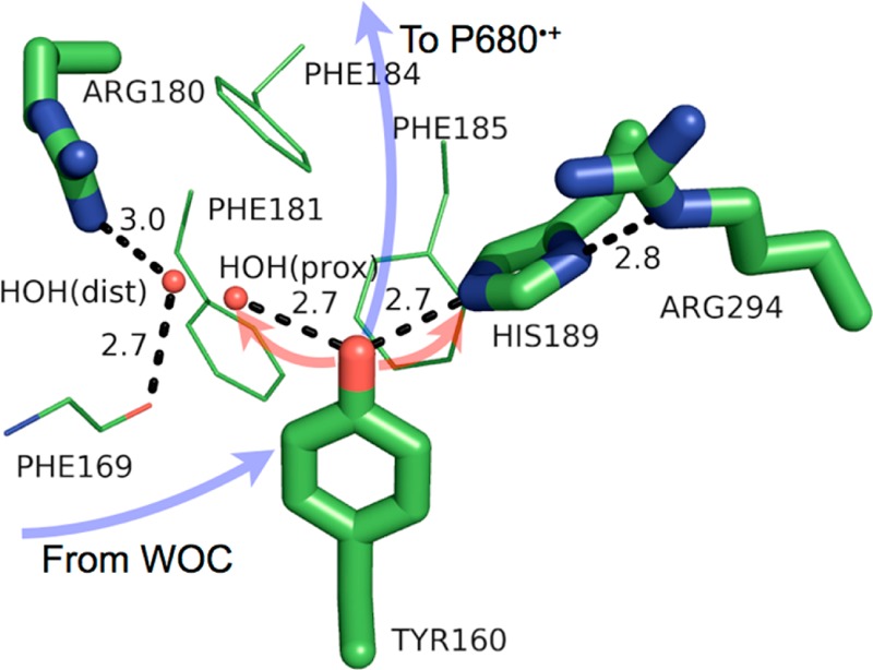
Model of the protein environment surrounding Tyr160 (TyrD) of photosystem II from T. vulcanus (PDB 3ARC). Distances shown (dashed lines) are in angstroms. Crystallographic waters [HOH(prox) = the “proximal” water, HOH(dist) = the “distal” water] are shown as small, red spheres. The directions of ET and PT are denoted by transparent blue and red arrows, respectively. The figure was rendered using PyMol.⁵⁴

TyrD so far contributes the following knowledge to PCET in proteins: (i) the protein may influence the direction of proton transfer in PCET reactions via H-bonding interactions secondary from the proton donor (e.g., D1-asparagine 298 vs D2-arginine 294); (ii) as for TyrZ, the pH of the surrounding environment—i.e., the protonation state of nearby residues—may change the mechanism of PCET; (iii) a largely hydrophobic environment can shield the TyrD-O^• radical from extrinsic reductants, leading to its long lifetime.

2.2. BLUF Domain

The BLUF (sensor of blue light using flavin adenine dinucleotide) domain is a small, light-sensitive protein attached to many cell signaling proteins—such as the bacterial photoreceptor protein AppA from Rhodobacter sphaeroides or the phototaxis photoreceptor Slr1694 of Synechocystis (see Figure 5). BLUF switches between light and dark states as a result of changes in the H-bonding network upon photoinduced PCET from a conserved tyrosine to the photo-oxidant flavin adenine dinucleotide (FAD).^6,13 Although the charge separation and recombination events happen quickly (less than 1 ns), the change in H-bonding network persists for seconds (see Figures 6 and 8).^6,68 This difference in H-bonding between Tyr8, glutamine (Gln) 50, and FAD is responsible for the structural changes that activate or deactivate BLUF.

Figure 5.

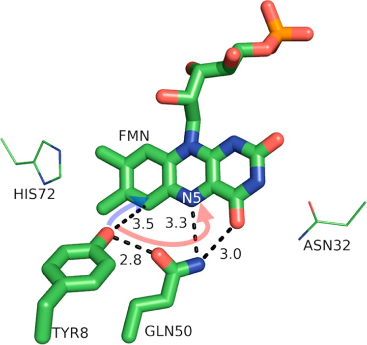
Model of the protein environment surrounding Tyr8 of the BLUF domain from Slr1694 of Synechocystis sp. PCC 6803 (PDB 2HFN). Distances shown (dashed lines) are in angstroms. N5 of the FMN (flavin mononucleotide) cofactor is labeled. The directions of ET and PT are denoted by transparent blue and red arrows, respectively. The figure was rendered using PyMol.⁵⁴

Figure 6.

Scheme depicting initial events in photoinduced PCET in the BLUF domain of AppA. Reprinted from ref (68). Copyright 2013 American Chemical Society.

Figure 8.

Model of the protein environment surrounding Tyr122 of ribonucleotide reductase from E. coli (PDB 1MXR). Distances shown (dashed lines) are in angstroms. Crystallographic water (HOH = water) is shown as a small red sphere, and the diiron sites are shown as large orange spheres. The directions of ET and PT are denoted by transparent blue and red arrows, respectively. The figure was rendered using PyMol.⁵⁴

The light and dark states of FAD are only subtly different, with FAD present in its oxidized form in both cases. For both dark and light states, photoinduced PCET, initiated via light excitation of FAD to FAD*, ultimaltely produces oxidized, deprotonated Tyr8-O^• and reduced, protonated FADH^•. However, this charge-separated state is relatively short-lived and recombines in about 60 ps.^6,13 The photoinduced PCET from tyrosine to FAD* rearranges H-bonds between Tyr8, Gln50, and FAD (see Figure 6), which persist for the biologically relevant time of seconds.^6,68,69 Perhaps not surprisingly, the mechanism of photoinduced PCET depends on the initial H-bonding network through which the proton might transfer; i.e., it depends on the dark or light state of the protein. Sequential ET and then PT has been demonstrated for BLUF initially in the dark state and concerted PCET for BLUF initially in the light state.^6,13 The PCET from the initial dark-adapted state occurs with an ET time constant of ∼17 ps in Slr1694 BLUF and PT occurring ∼10 ps after ET.^6,13 The PCET kinetics of the light-adapted state indicate a concerted ET and PT (the FAD^•– radical anion was not detected in the femtosecond transient absorption spectra) with a time constant of ∼1 ps and a recombination time of 66 ps.¹³ The concerted PCET may utilize a Grotthus-type mechanism for PT, with the Gln carbonyl accepting the phenolic proton, while the Gln amide simultaneously donates a proton to N5 of FAD (see Figures 5 and 7).¹³

Figure 7.

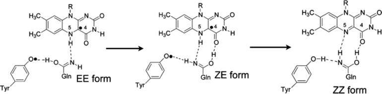
A possible scheme for H-bond rearrangement upon radical recombination of the photoinduced PCET state of BLUF. The energy released upon radical recombination may drive the uphill ZE to ZZ rearrangement. Adapted from ref (68). Copyright 2013 American Chemical Society.

Unfortunately, the nature of the H-bond network between Tyr–Gln–FAD that characterizes the dark vs light states of BLUF is still debated.^6,68,70 Some groups believe that Tyr8-OH is H-bonded to NH₂-Gln50 in the dark state, while others argue CO-Gln50 is H-bonded to Tyr8-OH in the dark state, with opposite assignments for the light state.^6,68,71 Surely, the H-bonding assignments of these states should exhibit the change in PCET mechanism demonstrated by experiment. Like PSII in the previous section, we see that the protein environment is able to switch the PCET mechanism. In PSII, pH plays a prominent role. Here, H-bonding networks are key.

The exact mechanism by which the H-bond network changes is also currently debated, with arguments for Gln tautomerization vs Gln side-chain rotation upon photoinduced PCET.^6,68,70 Radical recombination of the photoinduced PCET state may drive a high-energy transition between two Gln tautameric forms, which results in a strong H-bond between Gln and FAD in the light state (Figure 7).⁶⁸ Interestingly, when the redox-active tyrosine is mutated to a tryptophan, photoexcitation of Slr1694 BLUF still produces the FADH^• neutral semiquinone as in wild-type BLUF, but without the biological signaling functionality.⁷² This may suggest a rearrangement of the H-bonded network that gives rise to structural changes in the protein does not occur in this case.

What aspect of the H-bonding rearrangement might change the PCET mechanism? Using a linearized Poisson–Boltzmann model (and assuming a dielectric constant of 4 for the protein), Ishikita calculated a difference in the Tyr one-electron redox potential between the light and dark states of ∼200 mV.⁷¹ This larger driving force for ET in the light state, which was defined as Tyr8-OH H-bonded to CO-Gln50, was the only calculated difference between light and dark states (the pK_a values remained nearly identical). A larger driving force for ET would presumably seem to favor a sequential ET/PT mechanism. Why PCET would occur via a concerted mechanism if ET is more favorable in the light state is unclear. Further theoretical studies concerning an explicit theoretical treatment of the PCET mechanism (see section 5 and onward) are needed to clarify what gives rise to the switch from sequential to concerted PCET in BLUF domains.

What is unique about BLUF that gives rise to a Tyr radical cation, Tyr-OH^•+, whereas in PSII this species is not observed? We suggest the most important factor may be Coulombic stabilization. In general, the driving force for ET must take into account the Coulombic attraction of the generated negative and positive charges, E_C = (−14.4 eV)/(εR_DA), where ε is the dielectric constant and R_DA is the distance (Å) between the donor and acceptor. Tyr8-OH^•+ and FAD^•– are separated by 3.5 Å edge-to-edge, whereas TyrZ or TyrD of PSII is ∼32 Å from quinone A^•–. Further experimental and theoretical insight into the reason for radical cation formation is clearly necessary. The oxidation of Tyr8 to its radical cation form in BLUF is quite unusual from a biological standpoint and sets BLUF apart from other PCET studies concerning phenols.

While the BLUF domain is a convenient small biological protein for the study of photoinduced PCET and tyrosyl radical formation in proteins, it is far from a perfect “laboratory”. Structural subtleties across species affect PCET kinetics, and the environment immediately surrounding the Tyr radical cannot be manipulated without influencing the protein fold.⁷³ Nonetheless, BLUF is a valuable model from which to glean lessons toward the design of efficient PCET systems. The main ideas involving PCET from Tyr8 in BLUF are as follows: (i) PCET occurs via different mechanisms depending on the initial state of the protein (light vs dark). These mechanisms are either (a) concerted PCET from Tyr8 to FAD, forming Tyr8-O^• and FADH^•, or (b) sequential ET and then PT from Tyr8 to FAD, forming first FAD^•– and then FADH^•. (ii) The existence of a Tyr-OH^•+ radical cation has been argued against on energetic grounds for PSII TyrZ and TyrD. However, Tyr-OH^•+ was demonstrated experimentally for BLUF. (iii) More experimental and theoretical research is needed to elucidate the differences in dark and light states and the structural or dynamical differences that give rise to changes in the PCET mechanism depending on the Tyr8 H-bonding network.

2.3. Ribonucleotide Reductase

Ribonucleotide reductase (RNR) is a ubiquitous enzyme that catalyzes the conversion of RNA to DNA via long-distance radical transfer, which is initiated by the activation and reduction of molecular oxygen to generate a stable tyrosyl radical (Tyr122-O^•, t_1/2 = 4 days at 4 °C).^35,36 The formation of Tyr122-O^• is the first step in long-distance radical transfer across a protein dimer interface to the active site of nucleotide reduction. As such, the formation of Tyr122-O^• is perhaps one of the most important PCET reactions in nature. Its initiation is tightly coupled with redox states of the nearby nonheme dinuclear iron center.

Tyr122-O^• formation is a thermally induced, ground-state process (i.e., no photoexcitation is involved) and occurs slowly (1 s^–1) relative to phototriggered radical formation (ps, ns) of Tyr in proteins such as photolyase, PSII, and BLUF.^{14,19,75−77} Initiation of Tyr122-O^• involves dioxygen activation and reduction via a diiron center. Interestingly, the mechanism of Tyr122-O^• formation in catalytically competent RNR involves a Trp radical cation (vide infra). Trp48 reduction of Fe1(IV) to Fe1(III) produces the diiron intermediate Fe1(III)Fe2(IV) (denoted as X in the literature) responsible for the oxidation of Tyr122-OH.^75,76 In the oxidation of Tyr122-OH, the electron acceptor is Fe2(IV) (the more distant of the two irons) and the proton acceptor is a hydroxyl coordinated to Fe1.⁷⁸ The phenolic proton possibly transfers through Asp84, which forms a weak H-bond with Tyr122-OH (see Figures 9 and 10) in the met-RNR structure (met = Fe1(III)Fe2(III)).⁷⁴ There are currently no reported crystal structures of the catalytically active RNR, i.e., Fe1(III)Fe2(III)-Tyr122-O^•, so the H-bonding environment of the Tyr radical has been deduced via FTIR and EPR experiments (discussed below).

Figure 9.

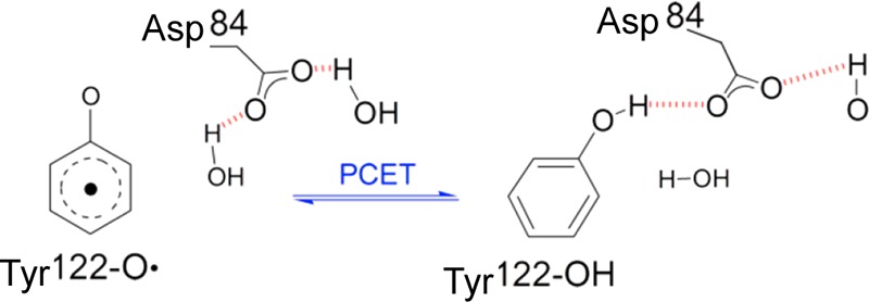
Schematic of the Asp84 H-bond shift, which is linked to Tyr122-O^• reduction (PCET). Adapted from ref (74). Copyright 2011 American Chemical Society.

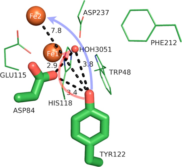
Figure 10.

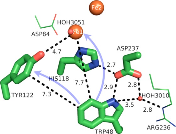
Model of the protein environment surrounding Trp48 of ribonucleotide reductase from E. coli (PDB 1MXR). Distances shown (dashed lines) are in angstroms. Crystallographic waters (HOH = water) are shown as small red spheres and the diiron sites as large orange spheres. The directions of ET are denoted by transparent blue arrows. The figure was rendered using PyMol.⁵⁴

The reduction and protonation of Tyr122-O^• in forward radical propagation to the cysteine active site (which is uphill in energy³⁵) is currently hypothesized to occur via Tyr356 (or Trp48) and the water coordinated to Fe1, respectively. PT to and from Tyr122 is therefore suggested to be a rocking mechanism, such as PT to/from TyrZ in PSII (where the proton rocks back and forth between TyrZ and D1-His190; see Figure 9 and section 2.1).^74,78 Because Tyr356 seems to be nearly isoenergetic with Tyr122 in terms of oxidation potential, the stability of Tyr122-O^• is apparently kinetic in nature, most likely due to PT gating enabled by protein conformational changes.³⁵

Radical propagation along the 35 Å hopping chain is proposed to occur in the microsecond time regime, although exact rates of each step are yet to be determined.³⁵ Time scales of radical transfer and identities of radical intermediates along the hopping pathway have been inferred via Tyr substitution of unnatural amino acids with altered redox potentials and pK_a values.^35,79 For instance, the reduction of an unnatural amino acid, NO₂-Tyr122-O^•, occurs in less than 1 ms, with the caveat that this reduction is not proton coupled (NO₂-Tyr122-O^•– is formed).^35,80 This ET uncoupled from PT might speed up the observed radical transfer kinetics by bypassing protein conformational gating of PT. Incidentally, the rate-limiting process for radical propagation is hypothesized to be protein conformational changes upon substrate and allosteric effector binding.³⁵

The nature of the Tyr122 H-bond appears to play an important role in radical formation and longevity. Tyr122 of class Ia RNR from Escherichia coli shares a hydrogen bond with Asp84, with R_O···O = 3.4 Å (see Figure 8). There is debate as to whether a water molecule acts as a H-bond intermediary between Tyr122 and Asp84, due to the long, observed H-bond distance and the fact that class Ib RNRs from other species contain an intermediary H-bonded water.⁷⁵ Numerical modeling of difference FTIR experimental data indicated the neutral radical form of Tyr122 (Tyr122-O^•) from E. coli is displaced by either 4 or 7 Å from its reduced, protonated form within met-RNR (PDB 1MXR).²⁸ Consequently, the Tyr122-O^• radical is not in a H-bonded environment (although in species other than E. coli the radical is in fact involved in H-bonding).^28,81,82 The absence of a discernible H-bond (due to rotation and translation of the radical away from Asp84 and the diiron cluster) and the relatively hydrophobic environment of Tyr122-O^•, which is dominated by the hydrophobic side chains of isoleucine and phenylalanine (see Figure 8 and Table 2), lead to its long lifetime (days).^36,75 Replacement of Tyr122 with a nitrotyrosine analogue in its hydrophobic pocket increased the analogue’s pK_a by >2.5 units, suggesting this hydrophobic environment plays a significant role in the PCET process.^35,83

Although the directionality of PT relative to ET has been inferred in RNR for various hopping steps (orthogonal PT/ET in the β subunit, collinear PT/ET in the α subunit), relatively little is known concerning the other PT steps along the radical transfer pathway. Furthermore, the PCET mechanism for generation of Tyr122-O^• may be a concerted or sequential PCET process, and further research is necessary to fully characterize this important radical formation.

PCET of Tyr122 in RNR has many parallels with PCET from TyrZ/D of PSII: (i) the phenolic proton is probably transferred back and forth via a rocking mechanism; (ii) Tyr-OH donates an electron in one direction (Fe2 for RNR, P680^•+ for PSII) and accepts an electron from another direction (Tyr356 or Trp48 for RNR, WOC for PSII); (iii) both Tyr122-O^• and TyrD-O^• reside in hydrophobic environments and have very long lifetimes (days and hours).

Tyr122 so far contributes the following knowledge to PCET in proteins: (i) protein conformational changes may be a means for PT gating and controlling radical transfer processes; (ii) elimination of H-bonding interactions in the radical state (Tyr122-O^•) by translocation away from a H-bonding partner provides a means for an increased radical lifetime; (iii) a largely hydrophobic environment can increase the pK_a of Tyr.

3. Tryptophan Radical Environments

Like Tyr radicals, Trp radicals are also major players in PCET processes in proteins, playing various roles in ribonucleotide reductase,^35,36 photolyase,^1,90 cytochrome c peroxidase,^91,92 and more. Similar to that of Tyr, the pK_a of Trp changes drastically following its oxidation (ΔpK_a^{Tyr/Tyr-OH•+} = 12, ΔpK_a^{Trp/Trp-H•+} = 13).¹⁰ However, the pK_a of neutral Trp-H (pK_a = 17) is high enough for its one-electron-oxidized form to remain protonated under physiological conditions (the pK_a of Trp-H^•+ is ∼4), and often, this is the case. Although proton management does not seem to be as vital for oxidation of Trp in proteins, PT still plays a large role in some cases. Studies of Trp oxidation in proteins may have particular relevance for guanine oxidation in DNA, where long-distance radical hopping along double- or single-stranded DNA has been experimentally demonstrated and theoretically investigated.⁹³⁻⁹⁵ In fact, a guanine radical in a DNA strand has been experimentally observed to oxidize Trp in a complexed protein.⁹⁶ Although Trp is one of the most easily oxidizable amino acids, it is still difficult to oxidize. Its generation and utilization along a hole-hopping pathway could preserve the thermodynamic driving force needed for chemistry at a protein active site. Below, we review a few proteins that produce Trp radicals to highlight features relevant for their design in de novo systems. Where appropriate, we point the reader to theoretical sections of this review to mark possible entry points to further theoretical exploration.

3.1. Ribonucleotide Reductase

Tryptophan 48 (Trp48) of class Ia RNR of E. coli is necessary for functionally competent RNR: its one-electron oxidation forms intermediate X (see section 2.3), which then establishes the Tyr122-O^• radical (with a rate of 1 s^–1).^75,76 Without Trp48 present as a reductant, the diferryl iron center oxidizes Tyr122, creating X-Tyr122-O^•, whose fate is dominated by nonproductive side reactions and, to a lesser extent, slow “leakage” (<0.06 s^–1) to the catalytically competent Fe1(III)Fe2(III)-Tyr122-O^• state.⁹⁷ The radical cation form of Trp48 (Trp-H^•+) is also capable of oxidizing Tyr122 directly, with a slightly faster rate than X (6 s^–1 vs 1 s^–1, respectively^36,76) and does so in the absence of external reductants.⁷⁶ Curiously, Fe1(IV) of the diferryl species oxidizes Trp48 and not the closer Tyr122 (see Figure 10), which would be thermodynamically easier to oxidize in water (i.e., Tyr has a lower redox potential in water at pH 7). This selectivity is perhaps an example of how proteins utilize proton management to control redox reactions.

Once intermediate X is formed by one-electron transfer from Trp48 to Fe1, Trp48-H^•+ is reduced by an external reductant (possibly a ferredoxin protein in vivo⁹⁸), so that the radical does not oxidize Tyr122-OH in vivo. Because Trp48-H is re-formed due to ET from an external reductant, yet another curiosity is that Tyr122-OH, and not Trp48-H, is oxidized by Fe2(IV) of X. Formation of intermediate X by oxidation of Trp48-H may lead to a structural rearrangement enabling efficient PT from Tyr122-OH to a bound hydroxyl. RNR might also control the kinetics by modulating the electronic coupling matrix element between the iron sites and these amino acids. Additionally, RNR may adopt an alternate conformation where Trp48 is actually closer to the diiron site than Tyr122. The precise reasons for the preferred oxidation of Trp48 by Fe1(IV) and Tyr122 by X are unknown.

Although Trp48 has been implicated in the long-distance radical transfer pathway of RNR,^36,99 its direct role in this hole-hopping chain is not yet confirmed.^35,100 Instead, the proposed radical transfer mechanism consists of all Tyr: (β)Tyr122-O^• → (β)Tyr356 → (α)Tyr730 → (α)Tyr731 → (α)cysteine 439 → reductive chemistry and loss of water. (α and β represent AAs found in the α and β subunits of the RNR dimer.) This radical transfer process is uphill thermodynamically by at least 100 mV, driven by the loss of water at the ribonucleotide substrate.¹⁰⁰ The back radical transfer, which re-forms Tyr122-O^•, is downhill in energy and proceeds rapidly.³⁵

The protein environment surrounding Trp48 appears to poise its function as a reductant. In the met structure of the RNR R2 subunit (diferric iron and unoxidized Tyr122-OH), Trp48 is surrounded by mainly polar AAs, as well as 14 waters within a 6 Å radius of its indole side chain (see Figure S6 in the Supporting Information and Table 2). The indole proton of Trp48 occupies a highly polar environment, immediately H-bonded to Asp237 (a conserved residue) and water 3010, which forms a H-bonding network with four more waters and Arg236 (Figure S6). The protonation state of the oxidized Trp48 was inferred from absorption spectroscopy, which displayed a spectrum characteristic of a Trp radical cation.⁷⁶ While proton transfer may not be involved in Trp48 oxidation, its H-bonding and local dielectric environment likely play important roles in modulating its redox potential for the facile reduction of the diferryl iron site to make intermediate X.³⁶ Indeed, mutation of Asp237 to asparagine resulted in loss of catalytic function, which may be explained either by loss of PT capability from Trp48 to Asp237 or by adoption of a different, nonviable protein conformation.¹⁰¹ Moreover, Trp48, Asp237, His118, and Fe1 form a motif similar to that found in cytochrome c peroxidase, where the ferryl iron is derived from a heme moiety (Figure 11).^36,102 This motif may provide a H-bonding network to position Trp48 preferentially for oxidation by Fe1(IV).

Figure 11.

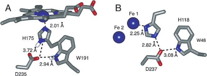
A common amino acid motif for the reduction of a ferryl iron. (A) The Asp, Trp, His motif of cytochrome c peroxidase produces Trp191-H^•+ and a heme-derived Fe(III). (B) The Asp, Trp, His motif of RNR produces Trp48-H^•+ (W48) and Fe(III) of intermediate X. Reprinted from ref (36). Copyright 2003 American Chemical Society.

There seem to be more open questions concerning Trp48 than there are answers: Fe1(IV) oxidizes Trp48-H and not Tyr122-OH, which is closer by 3 Å (see Figure 10). Why? Once established, Fe1(III)Fe2(IV) oxidizes Tyr122-OH and not Trp48-H. Why? Would knowledge of PCET matrix elements shed light on the preferences of these proton-coupled oxidations? The interested reader is referred to sections 5, 7, and 9–12 for an introduction and discussion of PCET matrix elements. Radical initiation in RNR highlights the intricate nature of PCET in proteins, which results from possible conformational changes, subtle H-bonding networks, perturbed redox potentials and pK_a values (relative to solution values), etc. More research is clearly needed to shed light on the vital Trp48 oxidation.

3.2. DNA Photolyase

3.2.1. Tryptophan 382

Photolyase is a bacterial enzyme that catalyzes the light-activated repair of UV-induced DNA damage, in particular the monomerization of cyclobutylpyrimidine dimers (CPDs).⁹⁰ Because photolyase is evolutionarily related to other FAD-binding proteins, such as cryptochromes, which share a conserved Trp hole-hopping pathway (Figure 12), insights regarding photolyase may be directly applicable to a wide variety of proteins.^1,103,104 The catalytic state of FAD, the anionic hydroquinone FADH^•–, donates an electron to the CPD in the first step of the DNA repair process after photoexcitation. FADH^•– is formed in vitro upon blue light photoexcitation of the semiquinone FADH^• and subsequent oxidation of nearby Trp382. Studying FAD reduction in E. coli photolyase, which could provide insight regarding signal activation via relevant FAD reduction of cryptochromes, Sancar et al. recently found photoexcited FAD* oxidizes Trp48 in 800 fs.¹ Hole hopping occurs predominantly via Trp382 → Trp359 → Trp306.^1,14,90 Oxidation of Trp306 involves proton transfer (presumably to water in the solvent, since the residue is solvent exposed), while oxidation of Trp382 generates the protonated Trp radical cation.^1,14 Differences in the protein environment and relative amount of solvent exposure are responsible for these different behaviors, as well as a nonzero driving force for vectorial hole transfer away from FAD and toward Trp306.^1,14

Figure 12.

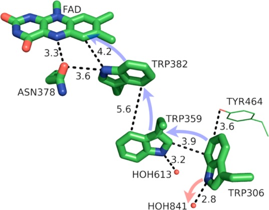
Model of the PCET pathway of photolyase from E. coli (PDB 1DNP). FAD (flavin adenine dinucleotide) absorbs a blue photon and oxidizes Trp382, which oxidizes Trp359, which oxidizes Trp306, which then deprotonates to the solvent. Crystallographic waters (HOH = water) are shown as small red spheres. The directions of ET and PT are denoted by transparent blue and red arrows, respectively. The figure was rendered using PyMol.⁵⁴

The three-step hole-hopping mechanism is completed within ∼150 ps of FAD photoexcitation.¹ Through an extensive set of point mutations in E. coli photolyase, Sancar et al. recently mapped forward and backward time scales of hole transfer (see Figure 13). The redox potentials shown in Figure 13 and Table 1 are derived from fitting the forward and backward rate constants to empirical electron transfer rate equations to estimate free energy differences and reorganization energies.¹ These redox potentials are based on the E_0,0 (lowest singlet excited state) energy of FAD (2.48 eV) and its redox potential in solution (−300 mV).¹ The redox potential of FAD in a protein may differ considerably from its solution value and has been shown to vary as much as ∼300 mV within LOV, BLUF, cryptochrome, and photolyase proteins.^73,103,105 However, these recent results emphasize the important contribution of the protein environment to establish a substantial redox gradient for vectorial hole transfer among otherwise chemically identical Trp sites.

Figure 13.

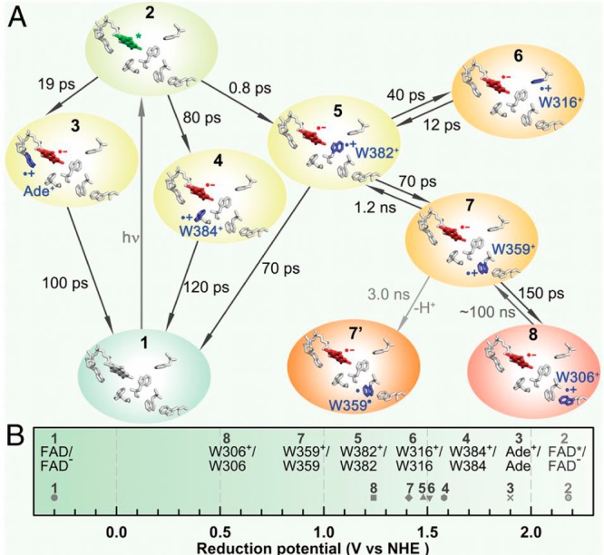
Time scales and thermodynamics of hole transfer in E. coli photolyase. Reprinted from ref (1).

The local protein environment immediately surrounding Trp382 is relatively nonpolar, dominated by AAs such as glycine, alanine, phenylalanine, and Trp (see Figure S7, Supporting Information). Although polar and charged AAs are present within 6 Å of Trp382, the polar ends of these side chains tend to point away from Trp382 (Figure S7). Trp382 is within H-bonding distance of asparagine (Asn) 378, although the long bond length suggests a weak H-bond. Asn378 is further H-bonded to N5 of FAD, which could suggest a mechanism for protonation of FAD to the semiquinone FADH^•, the dominant form of the cofactor (see Figure 12).¹⁰³ Interestingly, cryptochromes, which predominantly contain fully oxidized FAD (or one-electron-reduced FAD^•–), have an aspartate (Asp) instead of an Asn at this position. Asp could act as a proton acceptor (or participate in a proton-shuttling network) from N5 of FAD and so would stabilize the fully oxidized state.¹⁰³ Besides the long H-bond between Trp382 and Asn378, the indole nitrogen of Trp382 is surrounded by hydrophobic side chains. This “low dielectric” environment is likely responsible for the elevated redox potential of Trp382 relative to Trp359 and Trp306 (see Figure 13B), which are in more polar local environments that include H-bonding to water.¹

Trp382 so far contributes the following knowledge to radical formation in proteins: (i) elimination of H-bonding interactions with the indole side chain may increase the Trp oxidation potential, while still keeping the Trp side chain within a biologically useful redox window; (ii) gradients of amino acid polarity surrounding identical Trp cofactors can drive fast, vectorial hole transfer over long distances with a minimal driving force.

3.2.2. Tryptophan 306

Tryptophan 306 (Trp306) of E. coli photolyase (see section 3.2.1) is the terminal hole acceptor in a conserved hole transfer pathway consisting of three Trp residues (see Figure 12). Upon oxidation of Trp306, its deprotonation, presumably to water, occurs in ∼300 ns.¹⁴ Indeed, the crystal structure (Figure 12) indicates a water (HOH841) H-bonded to the indole nitrogen of Trp306 at a distance of 2.8 Å. By coupling the oxidation of Trp306 to proton loss, the lifetime of the charge-separated state is prolonged (17 ms).¹⁴ By studying the temperature dependence of the charge recombination reaction between FADH^•– and Trp306^•, Zieba et al. found a pH-dependent reorganization energy.⁸⁷ They infer that charge recombination between FADH^•– and Trp306^• is either sequential ET followed by PT (pH > 7, with a reorganization energy of ∼1.2 eV) or concerted PCET (pH < 7, with a reorganization energy of ∼2.2 eV).⁸⁷ Interestingly, they argue that these two mechanisms do not compete with each other kinetically; that is, a thermodynamic switch between them occurs, or a proton donor with a pK_a ≈ 6.5 becomes suddenly available. The charge recombination reaction, which occurs over a distance of 15 Å, deserves more theoretical attention, as it displays parallels with other known radicals with pH-dependent PCET mechanisms.

The local protein environment surrounding Trp306 is certainly more polar than that surrounding Trp382 (see Figures S7 and S8 in the Supporting Information and Table 2). Not only is Trp306 more solvent exposed, but most of the AAs within close proximity to Trp306 (e.g., aspartates 302 and 358 and threonines 388 and 301) are polar and/or charged. Trp306 so far contributes the following knowledge to PCET in proteins: (i) Trp oxidation coupled to proton loss is an efficient means to trap a radical and slow charge recombination; (ii) changes in the PCET mechanism must be considered at varying pH.

3.3. Azurin

The blue copper protein azurin from Pseudomonas aeruginosa has played a tremendous role in elucidating a quantitative understanding for the mechanisms of electron-tunneling, electron-hopping, and PCET pathways in proteins.^9,106−108 The Gray laboratory has exploited single histidine point mutations to label azurin with nonbiological Ru- and Re-based phototriggers.¹⁰⁹ These phototriggers, either through flash-quench methods or direct photooxidation, can initiate charge transfer reactions with the protein Cu redox center. Experiments from the Gray laboratory identified Trp122 as an effective hole shuttle between the electronically excited metal-to-ligand charge transfer (MLCT) triplet state of Re^I(CO)₃(dmp) (³[Re^II(CO)₃(dmp^•−)]*) and Cu(I), when Re is coordinated by histidine 124 (His124) (Figure 14).⁸⁸

Figure 14.

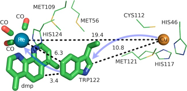
Model of the charge transfer pathway involving Trp122 of azurin from P. aeruginosa (PDB 2I7O) and the Re center of ³[Re^II(CO)₃(dmp^•−)]* coordinated at His124 (dmp = 4,7-dimethyl-1,10-phenanthroline). Distances shown (dashed lines) are in angstroms. The directions of ET are denoted by transparent blue arrows. The figure was rendered using PyMol.⁵⁴

Mutation of Trp122 to phenylalanine or tyrosine eliminated charge hopping, emphasizing the importance of redox potential modulation as well as management of coupled-proton transfers. Tyr oxidation is slightly more favorable thermodynamically than Trp oxidation if the ET is properly proton-coupled,¹⁰ so the absence of charge hopping with Tyr substitution suggests an appropriate proton acceptor for the phenolic proton is not present. The charge transfer mechanism of this modified azurin system, as well as its associated kinetic time scales, is shown in Figure 15. Rapid exchange between the electronically excited MLCT triplet state of Re^I(CO)₃(dmp) and the charge-separated state associated with oxidized Trp122 is responsible for the fast charge transfer (∼30 ns) between ³[Re^II(CO)₃(dmp^•–)]* and Cu(I), which are separated by 19.4 Å.^88,89 Hole hopping via Trp122 is the reason for the dramatic (∼300-fold) increase in the rate of Cu oxidation, since the distance from the mediating Trp122 is 6.3 Å away from the Re center and 10.8 Å from the Cu (see Figure 14). The short distance between Trp122 and Re allows for a rapid oxidation to generate Trp-H^•+ (<1 ns), mediated by the π–π interaction of the indole ring of Trp122 with dmp^•–. Despite its solvent exposure, Trp122 remains protonated throughout the charge-hopping process, possibly due to a longer time scale of Trp deprotonation to water (∼300 ns), as seen in the solvent-exposed Trp306 of E. coli photolyase (see section 3.2.2).¹⁴ Although Trp122 is solvent exposed, its protein environment is somewhat nonpolar, although polarizable with several methionine residues (see Figure S9 in the Supporting Information and Table 2).

Figure 15.

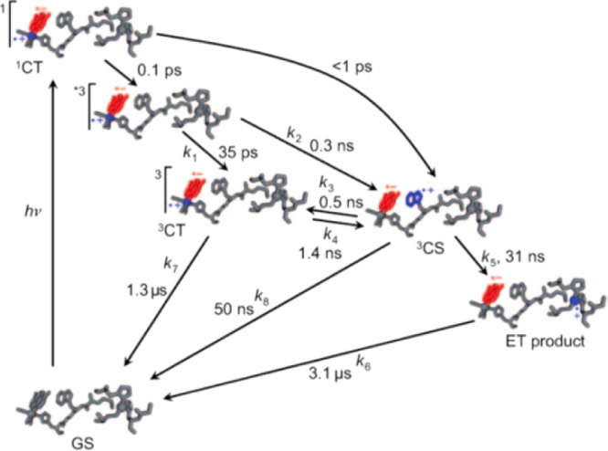
Kinetic scheme of photoinduced hole transfer from ³[Re^II(CO)₃(dmp^•–)]* to Cu(I) via the populated intermediate Trp122. The locations of the excited electron and hole are depicted in blue and red, respectively. Reprinted with permission from ref (89). Copyright 2011 Wiley-VCH Verlag GmbH & Co. KGaA.

What might this hole-hopping mediation via Trp122 teach us concerning PCET in proteins? Like in RNR, hole hopping is often kinetically advantageous when charge is transferred over long distances. Even modest endergonic hopping steps can be tolerated, as in the forward radical propagation of RNR, if the final charge transfer state is downhill in free energy. Fast charge hopping is an effective way to reduce the likelihood of charge recombination and is a tactic applied in PSII, although at the expenditure of a considerable amount of driving force.¹¹⁰ Certainly a timely topic of study is the elucidation of the criteria for rapid, photoinduced separation of charge with a minimal driving force. This azurin hopping system provides an interesting framework in which to study such events.

4. Implications for Design and Motivation for Further Theoretical Analysis

What have we learned from this overview of Tyr and Trp radical environments and their contributions to proton-coupled charge transfer mechanisms? The environments not only illustrate the significance of the local dielectric and H-bonding interactions, but also point toward design motifs that may prove fruitful for the rational design of bond breaking and catalysis in biological and de novo proteins. Indeed, de novo design of proteins that bind abiological cofactors is rapidly maturing.^111−113 Such methods may now be employed to study, in designed protein systems, the basic elements that give rise to the kinetic and thermodynamic differences of PCET reactions. Such systems may prove more tractable than their larger, more complicated, natural counterparts. However, design clues inspired by natural systems are invaluable.

Our discussion of Tyr and Trp radicals has emphasized a few, possibly important, mechanisms by which natural proteins control PCET reactions. For example, Tyr radicals in PSII show a dependence on the second H-bonding partner of histidine (His). While D1-His190 is H-bonded to TyrZ and Asn, D2-His189 is H-bonded to TyrD and Arg. The presence of the Arg necessitates His189 to act as a H-bond donor to TyrD, sending TyrD’s proton in a different direction (hypothesized to be a proximal water). Secondary H-bonding partners to His could thus provide a means to control the direction of proton translocation in proteins.

Physical movement of donors and acceptors before or after PCET events provides a powerful means to control reactivity. Tyr122-O^• has been shown to move several angstroms away from its electron and proton acceptors into a hydrophobic pocket where H-bonding is difficult. To initiate forward radical propagation upon substrate binding, reduction of Tyr122-O^• may be conformationally gated such that, upon substrate binding, the ensuing protein movement might organize a proper H-bonding interaction with Tyr122-O^• and Asp84 for efficient PCET. Indeed, TyrD-O^• of PSII may attribute its long lifetime to movement of a water after acting as a (hypothesized) proton acceptor. Movement of donors and acceptors upon oxidation can thus be a powerful mechanism for extended radical lifetimes.

The acidity change upon Trp oxidation can also be utilized in a protein design. The Trp-H^•+ radical cation is about as acidic as glutamic or aspartic acid (pK_a ≈ 4), so H-bonding interactions with these residues should form strong H-bonds with Trp-H^•+ (see section 1.2). Indeed, in RNR and cytochrome c peroxidase, we see this H-bonding interaction between the indole nitrogen of Trp and aspartic acid (Asp) (see Figures 10 and 11). The formation of a strong, ionic hydrogen bond (i.e., the H-bond donor and acceptor are charged, with matched pK_a values; see section 1.2) between Trp and Asp upon oxidation of Trp could provide an additional thermodynamic driving force for the oxidation.

Under what circumstances does Nature utilize Trp radicals vs Tyr radicals? The stringent requirement of proton transfer upon Tyr oxidation suggests that its most unique (and possibly most useful) feature is the kinetic control of charge transfer it affords via even slight changes in the protein conformation. Such control is most likely at play in long-distance radical transfer of RNR. Conversely, requirements for Trp deprotonation are not so stringent. If the Trp radical cation can survive for at least 0.5 μs, as in Trp306 of photolyase, a large enough time window may exist for reduction of the cation without the need for reprotonation of the neutral radical. In this way, Trp-H^•+ radicals may be useful for propagation of charge over long distances with minimal loss in driving force, as seen in photolyase.

Studying PCET processes in biology can be a daunting task. For instance, the PCET mechanism of TyrZ and TyrD of PSII depends on pH and the presence of calcium and chloride; the PCET kinetics of Tyr8 of BLUF domains depends on the species; fast PCET kinetics can be masked by slow protein conformational changes, as in RNR. Accurate determination of amino acid pK_a values in proteins is formidable due to the many titratable residues often present. Here, especially in the realm of PT, where convenient optical handles often associated with ET are absent, theory leads the way toward insight and the development of new hypotheses. However, profound theoretical challenges exist to elucidate PCET mechanisms in proteins. Accurate theoretical calculations of even the simplest PCET reactions are heroic efforts, where the theory is still under active development (see section 5 and onward). Naturally, larger more complicated biological systems provide an even greater challenge to the field of PCET theory, but these are the systems where theoretical efforts are most needed. For instance, accurate calculation of transition-state geometries would elucidate design criteria for efficient PCET in proteins.

There are clearly deep challenges and opportunities for the theory of PCET as it applies to biology. In the following part of this review, we aim to summarize and analyze the current status of the field of theoretical PCET (a burgeoning field with a rich past), as well as to examine interconnections with ET and PT theories. We hope to provide a focus such that the theory can be further developed and directed to understand and elucidate PCET mechanisms in their rich context of biology and beyond. Providing a unified picture of different PCET theories is also the first step to grasp their differences and hence understand and classify the different kinds of biological systems to which they have been applied. The starting point of this unified treatment is indeed simple: the time-independent and time-dependent Schrödinger equations give the equations of motion for transferring electrons and protons, as well as other relevant degrees of freedom, while the Born–Oppenheimer approximation, with its successes and failures, marks the different regimes of the transferring charge and environmental dynamics.

5. Coupled Nuclear–Electronic Dynamics in ET, PT, and PCET

Formulating descriptions for how electrons and protons move within and between molecules is both appealing and timely. Not only are reactions involving the rearrangements of these particles ubiquitous in chemistry and biochemistry, but these reactions also present challenges to understand the time scales for motion, the coupling of charges to the surrounding environment, and the scale of interaction energies. As such, formulating rate theories for these reactions challenges the theoretical arsenal of quantum and statistical mechanics. The framework that we review here begins at the beginning, namely with the Born–Oppenheimer approximation (given its central role in the development of PCET theories), describes theories for electron and atom transfer, and reviews the most recent developments in PCET theory due in great part to the contributions of Cukier, Hynes, Hammes-Schiffer, and their co-workers.

5.1. Born–Oppenheimer Approximation and Avoided Crossings

In molecular systems, the motion of all charged particles is strongly correlated, due to their Coulomb and exchange interactions. Nonetheless, many reactions produce a change in the average position of just a small number of these particles, so it is useful to formulate physical pictures and rate theories for the translocation of electrons and protons. To formulate theories of PT reactions, it is expedient to separate the dynamics of the transferring proton from the other nuclear degrees of freedom. This kind of separation is familiar, as it is the kind of separation accomplished with the ubiquitous Born–Oppenheimer (BO) approximation,^114,115 commonly used to separate electronic and nuclear motion. The analysis of PCET reactions is further complicated by the fact that the dynamics of the transferring electron and proton are coupled and, in general, cannot be separated via the BO approximation. Thus, investigating the regimes of validity and breakdown of the BO approximation for systems with concomitant transfer of an electron and a proton cuts to the core of the dynamical issues in PCET reactions and their description using available theoretical tools.

In this section, we review features of the BO approximation that are relevant to the study of PCET reactions. Concepts and approximations are explored to provide a unified framework for the different PCET theories. In fact, charge transfer processes (ET, PT, and coupled ET–PT) are consistently described in terms of coupled electronic and nuclear dynamics (including the transferring proton). To place PCET theories into a common context, we will also need a precise language to describe approximations and time scale separations that are made in these theories.

Including only the fundamental Coulombic interactions in the interaction potential energy of the PCET system, the Hamiltonian is written as

5.1

where T̂_Q is the nuclear kinetic energy operator, H(Q) is the electronic Hamiltonian, and Q ≡ {Q_α} denotes the set of nuclear coordinates or a (nuclear) reaction coordinate. The nuclear kinetic energy operator is

5.2

where P_α = −iℏ∇_α ≡ −iℏ∇_Qα is the momentum operator for the Q_α nuclear degree of freedom, with associated mass M_α. H includes the electronic kinetic energy

5.3

where p_i is the momentum operator for the ith electron of mass m, and the potential energy

5.4

which depends on the set of electronic coordinates q ≡ {q_i} and (parametrically after application of the BO separation) on Q.

The BO approximation separates the electronic and nuclear motion based on the large difference between m and M_α. Next, we examine the steps of the BO procedure,^114,115 focusing on PCET systems:

(i) The BO approach separates the nuclear and electronic degrees of freedom from the outset, by assuming that the wave function can be written as the product

5.5

of the vibrational wave function χ(Q) and the electronic wave function ϕ(Q,q). In the context of PCET systems, the coordinate of the transferring proton has a privileged role, which needs to be recognized in the form of the wave function, thus leading to further factoring of the BO product wave functions (used as basis functions to describe PCET systems). Indeed, in sections 5.2 and 5.3, the transferring proton’s coordinate R is defined, and Q denotes all of the remaining nuclear coordinates.

(ii) Fixing Q = Q̅, the nuclear kinetic energy is zero and the eigenvalues of are those of the electronic Hamiltonian H for the given nuclear coordinates and are provided by the time-independent Schrödinger equation for the electronic wave function:

5.6

This equation is solved for each fixed set of nuclear coordinates (“parametrically” in the nuclear coordinates), thus producing eigenfunctions and eigenvalues of H that depend parametrically on Q. Using eq 5.6 to describe coupled ET and PT events can be problematic, depending on the relative time scales of these two transitions and of the strongly coupled nuclear modes, yet the appropriate use of this equation remains central to most PCET theories (e.g., see the use of eq 5.6 in Cukier’s treatment of PCET¹¹⁶ and its specific application to electron–proton concerted tunneling in the model of Figure 43).

Figure 43.

Pathway for two-dimensional tunneling in Cukier’s model for electron–proton transfer reactions. Once the proton is in a position that symmetrizes the effective potential wells for the electronic motion (straight arrow in the left lower corner), the electron tunneling can occur (wavy arrow). Then the proton relaxes to its final position (after Figure 4 in ref (116)).

(iii) Equation 5.5 with ϕ(Q,q) obtained from eq 5.6 is substituted into the Schrödinger equation for the full system, yielding

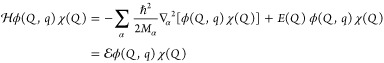5.7

(iv) At this point, the central approximation of the BO approach is made:

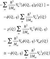5.8

This is the adiabatic approximation, which is based on the large difference in the electron and nuclear masses. This difference implies that the electronic motion is much faster than the nuclear motion, consistent with classical reasoning. In the quantum mechanical framework, applying the Heisenberg uncertainty principle to the widths of the position and momentum wave functions, one finds that the electronic wave function is spatially much more diffuse than the nuclear wave function.¹¹⁷ As a result, the electronic wave function is relatively insensitive to changes in Q_α and P_α (within the widths of the nuclear wave functions). That is, the electronic wave function can adjust quasi-statically to the nuclear motion.¹¹⁴ In the quantum mechanical formulation of eq 5.6, the concept of time scale separation underlying the adiabatic approximation is expressed by the neglect of the electronic wave function derivatives with respect to the nuclear coordinates (note that P_α = −iℏ∇_α).

The adiabatic approximation is, indeed, an application of the adiabatic theorem, which establishes the persistence of a system in an eigenstate of the unperturbed Hamiltonian in which it is initially prepared (rather than entering a superposition of eigenstates) when the perturbation evolves sufficiently slowly and the unperturbed energy eigenvalue is sufficiently well separated from the other energy eigenvalues.¹¹⁸ In its application here, the electronic Hamiltonian at a given time (with the nuclei clamped in their positions at that instant of time) plays the role of the “unperturbed” Hamiltonian. The change in the nuclear potential field, as nuclei move, acts as a perturbation that, de facto, changes the eigenstates and eigenvalues (thus making them time-dependent).

Substituting eq 5.8 into eq 5.7 and averaging on the electronic state, one finds

5.9

Equation 5.9 describes the behavior of the nuclear wave function in the effective potential E(Q), the electronic energy eigenvalue for fixed Q.

The terms omitted in the BO adiabatic approximation are generally non-negligible sufficiently near the Q values where the BO potential energy surfaces (PESs) are degenerate.¹¹⁴ Indeed, these crossing points define the geometries where charge transfer reactions are most likely to occur. Near curve crossings, the adiabatic separation usually fails, and one has to consider the dynamical effects of the moving nuclei on the electronic wave function. In this section, we review these nuclear dynamics effects on PESs, because they include the transition between electron donor and acceptor states that are coupled to nuclear motion corresponding to PT. Classical and quantum nuclear degrees of freedom are both considered in the analysis, which aims to establish a unified framework to describe the different PCET theories reviewed below.

Departure from the BO approximation means that the system can evolve among multiple BO wave functions of the form given in eq 5.5. Thus, the wave function Ψ of the system at a time t is expanded in a complete set of BO-type wave functions:

5.10

For simplicity, the time-dependent coefficients in eq 5.10 were incorporated into the vibrational functions.

The nuclear wave functions, for classical nuclei, are characterized approximately as δ functions. Hence, eq 5.10 for classical nuclei is

5.11

In this case, the nuclear motion is described in terms of classical trajectories Q(t), while the wave function description is limited to the electronic degrees of freedom by integrating eq 5.11 over Q to give

5.12

as in Tully’s formulation of molecular dynamics with hopping between PESs.^119,120 We now apply the adiabatic theorem to the evolution of the electronic wave function in eq 5.12.

For fixed nuclear positions, Q_α = Q̅_α, since the electronic Hamiltonian does not depend on time, the evolution of Φ from time t₀ to time t gives¹²¹

5.13

where

5.14

Taking into account the nuclear motion, since the electronic Hamiltonian depends on t only through the time-dependent nuclear coordinates Q(t), ϕ_n as a function of Q and q (for any given t) is obtained from the formally identical Schrödinger equation

5.15

The value of the basis function ϕ_n in q depends on time via the nuclear trajectory Q(t), so

5.16

Equation 5.16 describes the coupling between nuclear and electronic dynamics. That is, ϕ_n is not a stationary electronic state of the system Hamiltonian . In fact, while ϕ_n(Q(t₀),q) is an eigenfunction of the electronic Hamiltonian at time t₀, ϕ_n(Q(t₀),q) is not an eigenfunction of the electronic Hamiltonian at a later time t. The evolved wave function ϕ_n(Q(t),q) is, instead, an eigenfunction at this later time. Therefore, if the electronic state at time t₀ is described by a single wave function ϕ_n(Q(t₀),q), which implies that c_n′(t₀) = δ_n′n, other electronic wave functions appear in the system wave function Φ at later times, since the time evolution of the coefficients is described by the coupled differential equations¹¹⁹

5.17

Here, d_nk, known as the nonadiabatic coupling vectors,¹¹⁹ are

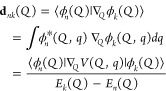5.18

(see the Supporting Information for a derivation). Equation 5.18 holds for k ≠ n (otherwise, d_nn = 0¹¹⁹) and

5.19

The matrix element in the numerator of the rightmost term in eq 5.18 describes the coupling between the wave functions ϕ_n and ϕ_k, at a given instant in time, due to the variation of V(Q,q); in fact, multiplication by Q̇ as in eq 5.19 transforms this matrix element into

5.20

For a given adiabatic energy gap E_k(Q) – E_n(Q), the probability per unit time of a nonadiabatic transition, resulting from the use of eq 5.17, increases with the nuclear velocity. This transition probability clearly decreases with increasing energy gap between the two states, so that a system initially prepared in state ϕ_n(Q(t₀),q) will evolve adiabatically as ϕ_n(Q(t),q), without making transitions to ϕ_k(Q(t),q) (k ≠ n).

Equations 5.17, 5.18, and 5.19 indicate that, if the nuclear motion is sufficiently slow, the nonadiabatic coupling may be neglected. That is, the electronic subsystem adapts “instantaneously” to the slowly changing nuclear positions (that is, the “perturbation” in applying the adiabatic theorem), so that, starting from state ϕ_n(Q(t₀),q) at time t₀, the system remains in the evolved eigenstate ϕ_n(Q(t),q) of the electronic Hamiltonian at later times t.

For ET systems, the adiabatic limit amounts to the “slow” passage of the system through the transition-state coordinate Q_t, for which the system remains in an “adiabatic” electronic state that describes a smooth change in the electronic charge distribution and corresponding nuclear geometry to that of the product, with a negligible probability to make nonadiabatic transitions to other electronic states.¹²² Thus, adiabatic states are obtained from the BO (adiabatic) approach by diagonalizing the electronic Hamiltonian. For sufficiently fast nuclear motion, nonadiabatic “jumps” can occur, and these transitions are more probable where two adiabatic states approach in energy, due to the increase in the nonadiabatic coupling vectors (eq 5.18). The adiabatic approximation at the core of the BO approach generally fails at the nuclear coordinates for which the zeroth-order electronic eigenfunctions are degenerate or nearly so. At these nuclear coordinates, the terms omitted in the BO approximation lift the energetic degeneracy of the BO electronic states,¹¹⁴ thus leading to splitting (or avoided crossings) of the electronic eigenstates. Moreover, the rightmost expression of d_nk in eq 5.18 does not hold at conical intersections, which are defined as points where the adiabatic electronic PESs are exactly degenerate (and thus the denominator of this expression vanishes).¹²³ In fact, the nonadiabatic coupling d_nk diverges if a conical intersection is approached¹²³ unless the matrix element ⟨ϕ_n|∇_QV(Q, q)|ϕ_k⟩ tends to zero.

Above, we considered electronic states that are zeroth-order eigenstates in the BO scheme. These BO states are zeroth order with respect to the omitted nuclear kinetic nonadiabatic coupling terms (which play the role of a perturbation, mixing the BO states), yet the BO states can serve as a useful basis set to solve the full dynamical problem. The nonzero values of d_nk encode all the effects of the nonzero kinetic terms omitted in the BO scheme. This is seen by considering the energy terms in eq 5.8 for a given electronic wave function ϕ_n and computing the scalar product with a different electronic wave function ϕ_k. The scalar product of ∇_αϕ_n(Q, q)·∇_αχ_n(Q) with ϕ_k is clearly proportional to d_nk. The connection between the magnitude of d_nk and the other kinetic energy terms of eq 5.8, omitted in the BO approximation and responsible for its failure near avoided crossings, is given by (see ref (124) and eqs S2.3 and S2.4 of the Supporting Information)

5.21

Thus, if d_nk is zero for each pair of BO basis functions, the latter are exact solutions of the full Schrödinger equation. This is generally not the case, and electronic states with zero or negligible couplings d_nk and nonzero electronic coupling

5.22

are instead searched for to construct convenient “diabatic” basis sets.^125,126 By construction, diabatic states are constrained to correspond to the precursor and successor complexes in the ET system for all Q. As a consquence, the dependence of the diabatic states on Q is small or negligible, which amounts to correspondingly small values of d_nk and of the energy terms omitted in the BO approximation.¹²⁷ For strictly diabatic states, which are defined by the

5.23

condition on nuclear momentum coupling,¹²⁸ the more general form of eq 5.17, that is¹¹⁹

5.24

takes the form

5.25

Therefore, according to eq 5.25, the mixing of strictly diabatic states arises exclusively from the electronic coupling matrix elements in eq 5.22. Except for states of the same symmetry of diatomic molecules, basis sets of strictly diabatic electronic wave functions do not exist, apart from the “trivial” basis set made of functions ϕ_n that are independent of the nuclear coordinates Q.¹²⁸ In this case, a large number of basis wave functions may be needed to describe the charge distribution in the system and its evolution accurately. Commonly adopted strategies obtain diabatic basis sets by minimizing d_nk values^12,129−133 or by identifying initial and final states of an ET process, considering the valence bond structures of the reactants and the products,¹²⁵ and using suitable computational techniques to reproduce these states.^134−146

Electronically diabatic states are degenerate at the transition-state coordinate, where the minimum energy (or free energy, after introduction of an ensemble of quantum states) gap between the corresponding adiabatic states (which can be obtained from a suitable linear transformation of the diabatic states^138,144) depends on the magnitudes of the electronic coupling matrix elements and, for nonorthogonal diabatic electronic states, on the overlaps among the diabatic states.^{134,135,138,141}

Diabatic states (reactant or initial ET state I and product or final ET state F) are considered in the theory of electron transfer,^7,147,148 where the transition-state coordinate(s) Q_t remains defined by the nuclear conformations at which the I and F “potential” (an effective potential) free energy surfaces (here denoted as PFESs; see the justification for this terminology in Appendix A) are degenerate.¹⁴⁹ In fact, the Franck–Condon principle and the requirement of energy conservation are simultaneously satisfied only for Q = Q_t. This observation, together with the assumptions of (a) identical polarization properties of reactants and products and (b) a linear response of the polarization of the solvent (which has the properties of a classical thermal bath with Gaussian statistics^150,151) to any charge change in the redox partners, led Marcus to a simple expression for the ET rate as a function of the reorganization (free) energy, λ, and the free energy of reaction ΔG_R° in the prevailing medium at a mean distance R between the ET partners in the activated complex.⁷

The Franck–Condon principle follows from the adiabatic approximation in the BO scheme. The BO scheme fails at Q_t. This failure persists after ensemble averaging, but it does not appreciably influence the expression for the activation free energy ΔG* in terms of λ and ΔG_R° in the Marcus rate constant as long as the avoided crossing of the adiabatic states amounts to a minimum energy gap much smaller than the activation barrier (see Figure 16a). The non-negligible coupling between nuclear and electronic dynamics near Q_t was introduced in the Marcus expression of the ET rate^152,153 in the semiclassical framework of Landau and Zener.^154−157 The Landau–Zener integration of the dynamical problem of eqs 5.22 and 5.25 over the region of the avoided crossing, together with the dependence of the ET rate on λ and ΔG_R° determined by Marcus and developed by Kubo and Toyozawa in the framework of nonradiative transitions of trapped electrons in crystals,¹⁵⁸ leads to the following nonadiabatic high-temperature expression for the ET rate (for classical nuclear degrees of freedom)¹⁵⁹ when the lifetime of the initial electronic state, τ_el ≈ ℏ/V_IF, is much larger than the time τ_n that the nuclei require to pass through the transition-state region, as determined by the parabolic shape of the Marcus PFESs (e.g., this is the case for very small electronic couplings):

5.26

Figure 16.

Cross section of the free energy profile along a nuclear reaction coordinate Q for ET. Frictionless system motion on the effective potential surfaces is assumed here.¹²⁶ The dashed parabolas represent the initial, I, and final, F, diabatic (localized) electronic states; Q_I and Q_F denote the respective equilibrium nuclear coordinates. Q_t is the value of the nuclear coordinate at the transition state, which corresponds to the lowest energy on the crossing seam. The solid curves represent the free energies for the ground and first excited adiabatic states. The minimum splitting between the adiabatic states approximately equals 2V_IF. (a) The electronic coupling V_IF is smaller than k_BT in the nonadiabatic regime. V_IF is magnified for visibility. λ denotes the reorganization (free) energy. (b) In the adiabatic regime, V_IF is much larger than k_BT, and the system evolution proceeds on the adiabatic ground state.

The Marcus form of the ET rate constant is

5.27

where ν_n is an effective nuclear frequency for motion along the reaction coordinate that allows the transition state to be reached and κ_el is the electronic transmission coefficient, given by

5.28a

with

5.28b

Equation 5.27 bridges the nonadiabatic regime and the adiabatic regime, where the electron transition probability at Q_t is unity and the ET rate takes the simple form (see Figure 16b)

5.29

The resulting Marcus–Levich–Dogonadze charge transfer theory is the basis of most PCET theories, motivating the attention given to this theory here.

The nonadiabatic coupling terms of the Schrödinger equation neglected in the BO approximation play a crucial role where charge transfer reactions are involved. In PCET, the transferring proton’s nuclear degrees of freedom need to be treated quantum mechanically. Hence, we reconsider the influence of the nonadiabatic interaction terms on the evolution of the system, writing the analogue of eq 5.24 for quantum nuclear degrees of freedom, which is relevant to a general description of PCET.

We first substitute the wave function of eq 5.10, for any given time (we use a complete set of real and orthogonal electronic basis functions and mass-weighted nuclear coordinates), into the time-independent Schrödinger equation. We then compute the scalar product with the nth electronic basis function, over the subspace spanned by the electronic degrees of freedom, obtaining^128,160

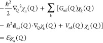5.30

Since Q̂ is a multiplicative operator in the coordinate representation, d_nk(Q) in eq 5.30 is still defined by the integral in eq 5.18; V_nk(Q) is defined by eq 5.22 so that V_nn(Q) = E_n(Q), and

5.31

By separating the diagonal and off-diagonal terms, one finds

5.32

which emphasizes the role of the electronic and nuclear coupling terms in eqs 5.22 and 5.31 in mixing otherwise adiabatic BO wave functions. The time-dependent Schrödinger equation is written by proceeding in a similar way and realizing that the time evolution of the nuclear state no longer appears in Q (which is now an eigenvalue of the observable Q̂), but in the pertinent wave functions:

5.33

Using a common notation,¹²⁵ eq 5.33 was written using wave functions χ_k that incorporate the time-dependent expansion coefficients of the wave function in terms of BO basis functions. Equation 5.33 is the analogue of eq 5.24 in the quantum case. |c_n(t)|² gives the probability of finding the system in the nth BO wave function, while |χ_n(Q,t)|² gives the probability density that the value of the nuclear coordinate is Q and the electrons are in state |ϕ_n(Q)⟩. The time derivative on the left side of eq 5.33 is the product of a time-independent nuclear vibrational function and the total time derivative of the nth expansion coefficient.

A detailed comparison of eqs 5.24 and 5.33 is absent in the literature, and it is beyond the scope of this review. However, useful insights into this comparison (which may be useful in the PCET context, where the reactive proton generally needs to be treated as a quantum mechanical particle, while other nuclear degrees of freedom can often be described using classical mechanics, unless they are directly coupled to the proton dynamics and are comparably fast) are provided by focusing on the off-diagonal energy terms related to the nuclear motion that are responsible for transitions between BO states.

The kinetic off-diagonal terms on the right-hand side of eq 5.33 describe two effects of the nuclear motion on the electronic state due to the interaction potential in eq 5.4. One term is the scalar product of ∇_Qχ_k, which is related to the quantum nuclear momentum, and d_nk, which is an expression of the change in the electronic wave function as a result of a change in the nuclear coordinates. In the perspective of the Lagrangian derivative (or material derivative),¹⁶¹ this off-diagonal term corresponds to the contribution that includes the “spatial derivative”.

The other off-diagonal term defined in eq 5.31 expresses a dependence of the electronic state on the nuclear kinetic energy. This is a kind of intrinsic dependence on the nuclear motion: in fact, if the same nuclear coordinates are associated with two different values of the nuclear kinetic energy, two different electronic states are accordingly obtained as a result of the interaction potential in eq 5.4. Therefore, the off-diagonal term arising from the fact that G_nk ≠ 0 would correspond to the “partial time derivative” in the material derivative of the Lagrangian picture. Note that this term is present even if the nth and kth electronic states are associated with the same vibrational function, and it is absent in the limit of classical nuclear motion, where a given electronic state corresponds to a given set of nuclear coordinates and Q(t) acts as a changing “external” field on the electronic wave function given by eq 5.12, thus yielding the coupling Q̇·d_nk in eq 5.24, to be compared with the analogous term in eq 5.33.

Note that, in both the quantum and the semiclassical cases, the nonadiabatic couplings that arise from nuclear motion are zero or negligible for any suitable set of diabatic states (by construction of the latter), so eqs 5.32 and 5.33 become

5.34

and

5.35

respectively. Near each minimum in Figure 16 one of the diabatic states is indistinguishable from the adiabatic ground state. The interaction between the electron donor and acceptor is negligible near a PES minimum where such a minimum is deep enough to be a feature of the PES landscape. In other words, if the system is near the bottom of a sufficiently deep PES minimum, the reactive electron is localized around a trapping donor (acceptor) site, and the electron localization is virtually indistinguishable from that for the isolated donor (acceptor) site. Therefore, the strictly diabatic electronic state defined as independent of the nuclear coordinates and equal to the adiabatic state at the coordinates of the minimum is, within the BO scheme, a zeroth-order eigenstate of the unperturbed electronic Hamiltonian for the reactant or product species corresponding to that minimum. The reactant (product) Hamiltonian is obtained (a) by partitioning the ET system to distinguish donor and acceptor groups, with the transferring charge included in the donor (acceptor), (b) by writing the energy as a sum of the energies of the single components plus their interactions, and (c) by removing the interaction between the donor and acceptor, which is responsible for the transition. These are known as “channel Hamiltonians”.^{126,127,159,162} An example is provided by and in eq 9.2.

Only the off-diagonal interaction terms (which determine the transitions according to eq 5.32) are removed from channel Hamiltonians.¹⁵⁹ In fact, considering an electronic state localized on the donor or acceptor, a diagonal term such as G_nn in eq 5.32 represents the interaction between the electron described by the localized wave function ϕ_n(Q,q) and the environment (before or after the transition), acting on ϕ_n through the kinetic energy operator −ℏ²∇_Q²/2. In short, using channel Hamiltonians, the interaction terms causing the charge transition are removed from the Hamiltonian (with the excess electron in the donor or acceptor group), and then its eigenfunctions can be searched. This is an alternative to working on the differential properties of the wave functions^{123,128,129,133,163} to obtain diabatic states, by seeking, for example, unitary adiabatic-to-diabatic transformations that minimize the nuclear momentum coupling.^133,163

5.2. Adiabatic and Nonadiabatic (Diabatic) Behavior in PCET

When the nuclear motion (or, more generally, the motion of heavy particles such as atoms or entire molecules where only the transferring electrons and/or protons need to be treated quantum mechanically) is sufficiently slow or when the nuclear coupling terms are negligible compared to the electronic couplings V_nk, the electron subsystem responds instantaneously to such a motion. An example is depicted in Figure 16b, where (a) the atoms are treated classically, (b) d_nk = 0 for the given diabatic states, and (c) the large value of the electronic coupling V_nk implies that the system evolves on the initially populated adiabatic electronic state. Thus, the adiabatic states are good approximations of the eigenstates of H at any time, and at position Q_t the system transits with unit probability to the product basin. In other words, when the system is at Q_t, depending on the adiabatic or diabatic nature (hence, on the localization properties) of the state in which the electronic subsystem was initially prepared, the transferring electron charge remains in the lower adiabatic state, or switches to the product diabatic state without lingering in the initial diabatic state (note that the two effective potential energy basins involved in the charge transition belong to the same adiabatic state, but to different diabatic, or localized, states), thereby promoting the subsequent nuclear relaxation to the equilibrium nuclear structure of the products. Figure 16a or 17 (see also ref (159), p 109) shows the opposite nonadiabatic regime, where the electronic charge distribution does not respond instantaneously to the nuclear motion.

Figure 17.

Multiple passage at Q_t, crossing of the reactant and product PFESs in nonadiabatic charge transfer. If the electronic coupling between the two diabatic states corresponds to a small Landau–Zener parameter, the system lingers in the initial diabatic electronic state I, rather than passing to the final state F at the first attempt. In fact, the formulation of this multiple crossing between the I and F surfaces by Landau and Zener gives rise to the expression for the electronic transmission coefficient in eq 5.28, which is proportional to the square coupling in the nonadiabatic limit, as in eq 5.26, and is unity in the adiabatic limit, as in eq 5.29.

The BO separation can be applied in different ways for different PCET reactions in solution. The electronic transition can be nonadiabatic with respect to both the motion of the heavy particles that are treated classically (solvent reorientation and motion of solute atoms that are not involved in proton or atom transfer) and the motion of the transferring proton(s) that is (are) treated quantum mechanically, or the electronic system may follow the first motion adiabatically and the second motion nonadiabatically¹⁶⁴ and so forth. Similarly, proton transfer reactions can be classified as either adiabatic or nonadiabatic with respect to the other nuclear coordinates.^165−167 Thus, a general theory that can capture different regimes of PCET needs to include the possibility of distinguishing between nuclear degrees of freedom with classical and quantum behavior and to properly model the interplay of different time scales and couplings that generally characterize PCET reactions.

In moving the above analysis toward more direct application to PCET systems, we consider a system where the coordinate R in the set Q behaves in a special way. R is the coordinate for a proton that will undergo a transition in a PCET reaction mechanism (more generally, R may be a set of nuclear coordinates that include other degrees of freedom critical for the occurrence of the reaction). We now use the symbol Q to denote the set of generalized coordinates of the heavy atoms other than R. For simplicity, we use the harmonic approximation and hence normal modes, so that the vibrational wave functions belonging to the nth electronic state can be factored as χ_n^p(R) χ_n(Q). We begin with this simple model to further dissect and clarify key concepts that emerge from theories of PCET.

Consider a complete set (or a nearly complete set, i.e., a set that is large enough to provide a good approximation of the system state at any time during the reaction) of electronically diabatic wave functions:

5.36

In eq 5.36, the electronic wave functions may be defined as ϕ_n(R,Q,q) = ϕ_n(R_n,Q_n,q), where (R_n,Q_n) is the minimum point of the pertinent free energy basin (this definition amounts to the use of strictly diabatic electronic states) or ϕ_n may have a weak dependence on the nuclear coordinates, thus being an approximate diabatic function. We have ∇_{R,Q} = ∇_R + ∇_Q, and, since R and Q are orthogonal coordinates, ∇_{R,Q}² = ∇_R² + ∇_Q². Thus, eq 5.34 is

5.37

In the electronically nonadiabatic limit (i.e., for V_nk → 0), each diabatic surface is identical with an adiabatic one, except for the small (vanishing, as V_nk shrinks) regions of the conformational space where different diabatic states are degenerate and the corresponding adiabatic states avoid the crossing because of the nonadiabatic kinetic coupling terms. This is seen from eq 5.37, which in the limit V_nk → 0 produces the Schrödinger equation for the nuclear wave function within the BO scheme.

If the large set of “bulk” nuclear coordinates (Q) can be replaced by a single reactive coordinate, one obtains a two-dimensional representation of the nuclear conformational space, as illustrated in Figure 18, where the minima of the PFESs correspond to reactants and products in their equilibrium conformations. The two minima are separated by a barrier, which is the activation barrier for the transition. The minimum value of the barrier on the crossing seam of the two PESs is a saddle point for the lower adiabatic PES, which is essentially identical to one of the diabatic states around each minimum. In a classical description of the nuclei, the reaction path matches the direction of the gradient at each point of the lower adiabatic PES. A curvilinear abscissa along the reaction path defines the reaction coordinate, which is a function of R and Q, and can be usefully expressed in terms of mass-weighted coordinates (as a specific example, a straight-line reaction path is obtained for crossing diabatic surfaces described by paraboloids).^168−172 This is also the trajectory in the R, Q plane according to Ehrenfest’s theorem. Figure 16a gives the PES (or PFES) profile along the reaction coordinate. Note that the effective PES denoted as the initial one in Figure 18 is indistinguishable from the lower adiabatic PES below the crossing seam, while it is essentially identical to the higher adiabatic PES above the seam (and not very close to the crossing seam, up to a distance that depends on the value of the electronic coupling between the two diabatic states). Similar considerations apply to the other diabatic PES.

Figure 18.

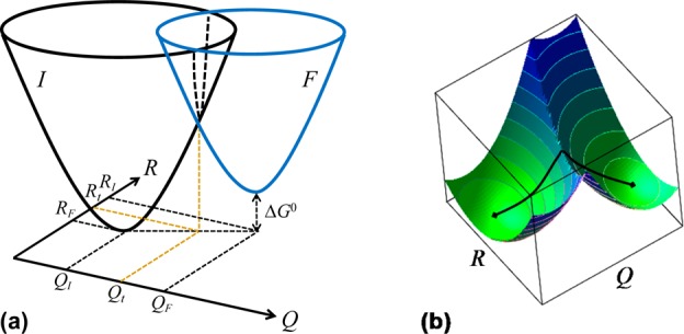
(a) Diabatic free energy surfaces before (I) and after (F) ET plotted as functions of the proton (R) and collective nuclear (Q) coordinates. If ΔR = R_F – R_I is larger than the proton position uncertainty in its initial and final quantum states, ET is accompanied by PT. Initial-, final-, and transition-state nuclear coordinates are marked, similar to the one-dimensional case of Figure 16. A dashed line describes the intersection of the two diabatic surfaces. (b) Adiabatic ground state. In the nonadiabatic limit, this adiabatic state is indistinguishable from the lower of the two diabatic free energy surfaces on each side of the crossing seam. In the opposite adiabatic regime, the adiabatic ground state significantly differs from the diabatic surfaces and the motion of the system occurs only on the ground-state free energy surface.

The possible transition dynamics between the two diabatic states near the crossing seams can be addressed, e.g., by using the Tully surface-hopping¹¹⁹ or fully quantum¹²⁵ approaches outlined above. Figures 16 and 18 represent, indeed, part of the PES landscape or circumstances in which a two-state model is sufficient to describe the relevant system dynamics. In general, a larger set of adiabatic or diabatic states may be required to describe the system. More complicated free energy landscapes characterize real molecular systems over their full conformational space, with reaction saddle points typically located on the shoulders of conical intersections.^173−175 This geometry can be understood by considering the intersection of adiabatic PESs related to the dynamical Jahn–Teller effect.¹⁷⁶

A typical PES profile for ET is illustrated in Figure 19b and is related to the effective potential seen by the transferring electron at two different nuclear coordinate positions: the transition-state coordinate x_t in Figure 19a and a nuclear conformation x̅ that favors the final electronic state, shown in Figure 19c. ET can be described in terms of multielectron wave functions differing by the localization of an electron charge or by using a single-particle picture (see ref (135) and references therein for quantitative analysis of the one-electron and many-electron pictures of ET and their connections).^141,177 The effective potential for the transferring electron can be obtained from a preliminary BO separation between the dynamics of the core electrons and that of the reactive electron and the nuclear degrees of freedom: the energy eigenvalue of the pertinent Schrödinger equation depends parametrically on the coordinate q of the transferring electron and the nuclear conformation x = {R,Q}¹¹⁶ (indeed x is a reaction coordinate obtained from a linear combination of R and Q in the one-dimensional picture of Figure 19). This is the potential V(x,q) represented in Figure 19a,c. At x = x_t, the electronic states localized in the two potential wells are degenerate, so that the transition can occur in the diabatic limit (V_nk → 0) by satisfying the Franck–Condon principle and energy conservation. The nonzero electronic coupling splits the electronic state levels of the noninteracting donor and acceptor. At x = x_t the splitting of the adiabatic PESs in Figure 19b is 2V_nk. This is the energy difference between the delocalized electronic states in Figure 19a. In the diabatic picture, the common energy of the two localized levels is E_j(x) = ⟨ϕ_j(x)|V(x,q) + T̂_q|ϕ_j(x)⟩ and represents the effective potential for the motion of the nuclei at x_t in each of the electronic states localized near the donor and acceptor.

Figure 19.

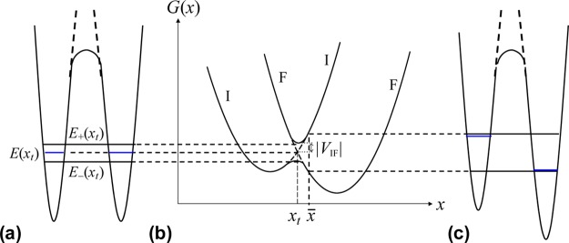
(a) Effective potential energy V(x_t,q) (q is the reactive electron coordinate) for the electronic motion at the transition-state coordinate x_t. x is a reaction coordinate that depends on R and Q. The energy levels corresponding to the initial and final electron localizations are degenerate at x_t (see blue bars in the figure). Denoting the diabatic electronic states by |ϕ_I,F(x)⟩, which depend parametrically on x, E(x_t) = E_I(x_t) = ⟨ϕ_I(x_t)|V(x_t,q) + T̂_q|ϕ_I(x_t)⟩ = E_F(x_t). However, such levels are split by the tunnel effect, so that the resulting adiabatic energies are E_± and the corresponding wave functions are equally spread over the electron donor and acceptor. (b) The effective potential (free) energy profile for the motion of the nuclear coordinate x is illustrated as in Figure 16. (c) An asymmetric effective potential energy V(x̅,q) for the electron motion at a nuclear coordinate x̅ ≠ x_t with accordingly asymmetric electronic levels is shown. The additional splitting of such levels induced by the tunnel effect is negligible (note that the electronic coupling is magnified in panel b). The black bars do not correspond to orbitals equally diffuse on the ET sites.

The introduction of a “special” coordinate R, useful in tackling multiple charge and/or atom transfer mechanisms, brings intricacies to the dynamics, as well as new meaning and significance for the one-dimensional PESs of Figures 16 and 19, as was discussed by Dogonadze, Kuznetsov, and Levich, who examined the possibility of a second adiabatic approximation separating R and Q in the same spirit of the BO scheme^178−180 (see below). In their approach, R was the coordinate for a proton involved in hydronium ion neutralization (discharge) at a metal surface¹⁷⁹ or in PT in solution.¹⁸⁰ The effective potential energy in the standard BO equation for the nuclei (namely, the electronic state energy as a function of the nuclear coordinates, or electron term) was written as a power series of the small deviations of the nuclear coordinates from equilibrium, up to second-order terms. A separate coordinate was assigned to the proton and the procedure was repeated, thus introducing a second adiabatic approximation for the proton with respect to slower degrees of freedom.

Kuznetsov and Ulstrup further developed these concepts¹⁸¹ by focusing directly on the energy terms contributing to the electronic or electron–proton PESs and averaging these PESs over the electronic and vibrational states. This procedure was accomplished in the diabatic electronic representation for the case of electronically nonadiabatic PT. Instead, an adiabatic electronic state representation was used in the electronically adiabatic regime. In this regime (quantum mechanical) averaging over the proton states to obtain electron–proton free energy surfaces (or electron–proton terms¹⁸⁰) is not appropriate. In fact, the proton wave functions that correspond to an adiabatic electronic state do not represent proton localization in the reactant or product wells, but rather are linear combinations of the localized proton vibrational functions. Thus, proton state averaging is no longer suitable in the electronically and vibrationally adiabatic case, where also the PT reaction occurs adiabatically with respect to the environment nuclear degrees, or in the electronically adiabatic and vibrationally nonadiabatic case, where this averaging does not lead to electron–proton free energy surfaces describing the proton localizations before and after PT (but rather to their mixtures; see the discussion of Figure 23). Thus, the two-dimensional nuclear space of Figure 18b is maintained in the partially and fully adiabatic regimes.

Figure 23.

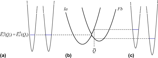
Analogue of Figure 19 for nonadiabatic EPT. The vibronic free energy surfaces are indicated in the central panel as functions of the collective coordinate Q. Panels a and c represent proton effective PESs (hence, they are drawn along the proton coordinate R) for Q = Q_t and Q = Q̅ ≠ Q_t, respectively. In the first case, E_I,F(R,Q_t) = ⟨ϕ_I,F(R,Q_t)|V(R̂,Q_t,q̂) + T̂_q|ϕ_I,F(R,Q_t)⟩ and the vibrational energies are, in both wells, ⟨χ_I^a|E_I(R,Q_t)|χ_I⟩ + T_I^a = E̅_I(Q_t) = E̅_F^b(Q_t). The two minima in panel a need not be equally deep if states a and b are not both ground vibrational states (cf. Figure 44).

These previous studies were further developed to treat different kinds of PCET mechanisms (e.g., see ref (182) and references therein). Nevertheless, PCET theories and applications have been developed much further.^182−186 We continue our analysis of Schrödinger equation applications with the aim of highlighting these developments.

We described the separation of electronic and nuclear dynamics above, focusing mainly on electronically nonadiabatic reactions. In Figure 18, the electron and proton motions are assumed to depend on the rearrangements of the same nuclear coordinate Q, as in Cukier’s treatment of PCET, for example.^{116,187−190} In this kind of model, where the same change in Q triggers both ET and PT events, if the (proton-coupled) ET reaction is in the nonadiabatic regime, the associated PT reaction is necessarily electronically nonadiabatic,^{165,182,190−193} as discussed in the following section. However, in many circumstances, electronically adiabatic PT may be coupled to nonadiabatic ET in the PCET reaction. This may be the case for well-separated electron donor and acceptor linked by a H-bonded interface that is involved in the PT.¹⁹⁴ In this case, the electronic charge distributions corresponding to the initial and final proton states are strongly coupled. In other words, due to the short PT distance, the electronic charge distribution can respond quickly to the proton motion.

It is worth stressing that the definition of electronically adiabatic or nonadiabatic PT is more general than its application to simultaneous ET and PT processes. In fact, this definition rests directly on the BO adiabatic approximation, and hence, it also applies when the electron charge rearrangement following the PT reaction is not classified as ET because it does not amount to distinct localizations of some excess electronic charge (see also the extended interpretation of the Dogonadze–Kuznetsov–Levich model in section 9). The electronic adiabaticity/nonadiabaticity criteria for the proton transition have been described¹⁹⁵ for simultaneous (or concerted) electron–proton transfer (also referred to as EPT in the literature^4,196 and in this review) and hydrogen atom transfer (HAT),^195,197 using an approximate description of the proton tunneling via Gamow’s formulation¹⁹⁸ (with the WKB approximation^199−202), a convenient definition of a “tunneling velocity” and the related “tunneling time” for the proton, and the Landau–Zener formalism¹⁵⁹ (see section 7). The synchronized electron and proton transitions can also involve the same donor and different acceptors or different donors and a common acceptor, which defines the multiple-site electron–proton transfer (MS-EPT) and the concept of PCET pathways.⁴ In a free energy landscape such as that of Figure 18, the change in R between two minima is a measure of the change in proton localization, while the change in Q reflects the rearrangement of the nuclei in response to the double charge transfer.

In general, the ET reaction occurs between donor and acceptor groups that are different from the ones involved in the PT event. The reaction may be concerted or stepwise (but the two transitions are nonetheless coupled, so that one induces the other, when PCET is at play), as is the case for many PCET mechanisms involving enzymes^4,203−208 and transition-metal complexes.^4,209−213

PCET reactions can fall into three different regimes of adiabatic or nonadiabatic behavior if, in evaluating the adiabaticity of the electronic state evolution, one considers the motion of the transferring proton and of the other nuclear degrees of freedom separately. These regimes are electronically adiabatic PT and ET, electronically nonadiabatic PT and ET, and electronically adiabatic PT and electronically nonadiabatic ET.^184,191,194 The electronically nonadiabatic or adiabatic character of the PT reaction refers to the relative time scales of the electron and proton dynamics, while the nonadiabatic or adiabatic behavior of the electronic motion is established with respect to all of the nuclear modes, therefore including the transferring proton.

Locally, the electronic motion is always much faster than the motion of the proton and of any other nuclear degree of freedom. In particular, this consideration applies to the electronic charge rearrangement that accompanies any pure PT or HAT event. However, when EPT occurs, the electronic charge rearrangement coupled to the PT involves (by the definition of ET) distinguishable (i.e., well-separated) initial and final electronic charge distributions. Thus, depending on the structure of the system (and, in particular, depending on the electron donor–acceptor distance), the PT is electronically adiabatic or nonadiabatic. With these considerations, one can understand why (electronically) adiabatic ET implies electronically adiabatic PT (overall, an electronically adiabatic double-charge transfer reaction) for both the stepwise and concerted electron–proton transfer reactions. Consider the four diabatic electronic states involved in a PCET reaction:^116,214,215

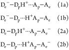5.38

where a and b denote the initial and final states of the PT process, 1 and 2 denote the ET states, and D_p (D_e) and A_p (A_e) denote the proton (electron) donor and acceptor, respectively. The possible charge-transfer processes connecting these states are shown in Figure 20. Pure PT occurs over short distances where the electron charge rearrangement between the initial and final states is adiabatic. Thus, if ET/PT (PT/ET) takes place, the proton transfer step PT₁ (PT₂) is electronically adiabatic. Since we are considering adiabatic ET (hence, the ET_a or ET_b step is also adiabatic by hypothesis), the full reaction is electronically adiabatic. Next consider the case in which EPT is the operational mechanism. The adiabatic behavior of the ET reaction is defined, according to the BO approximation, with respect to the dynamics of all nuclear degrees of freedom, hence also with respect to the proton transfer.¹⁹⁵ Thus, in the EPT mechanism with adiabatic ET, the PT process occurs on an adiabatic electronic state, i.e., it is electronically adiabatic.

Figure 20.

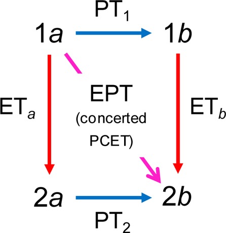
Possible realizations of a PCET mechanism (eq 5.38). The overall reaction is described by one of the following mechanisms: ET in the initial proton state a (ET_a) followed by PT in the final electronic state 2 (PT₂) (overall, an ET/PT reaction); PT in the initial electronic state 1 (PT₁) followed by ET in the final proton state b (ET_b), namely, a PT/ET reaction; simultaneous EPT to different or identical charge donor and acceptor (therefore, in this diagram HAT is included as a special case of EPT, although the acronym EPT is often used to denote distinguishable redox partners for ET and PT). On the whole, PCET can occur: as ET_a, where the process is coupled to the next occurrence of PT; as ET_b, where ET is triggered by the preceding PT; in conjunction with PT in an EPT or HAT reaction.

If the proton motion is sufficiently fast compared to the other nuclear degrees of freedom, the double-adiabatic approximation applies, which means that the PT proceeds adiabatically (adiabatic PT^165−167 or vibrationally adiabatic PT^182,191). Otherwise, nonadiabatic or vibrationally nonadiabatic PT is at play. These concepts are embodied in eqs 5.36 and 5.37. The discussion in the next section analyzes and extends the modeling concepts underlying eqs 5.36 and 5.37.

5.3. Adiabatic and Nonadiabatic PCET Interpreted in the Context of the Schrödinger Equation and the Born–Oppenheimer (Adiabatic) Approximation

In this section we analyze the coupled evolution of the reactive electron, the reactive proton, and the environment reaction coordinate(s) Q of a PCET system. The analysis uses a common theoretical framework for the coupling of electronic and nuclear dynamics that leads to adiabatic or nonadiabatic behaviors in ET, PT, and PCET. This perspective combines theoretical features from previous separate studies of these charge transfer reactions.

5.3.1. Quantum-State Dynamics of PCET Systems and the Underlying Potential (Free) Energy Surfaces

Our analysis begins with the definition of a general form for the quantum state of a PCET system and its quantum equations of motion. Because PCET reactions are common with long-range (nonadiabatic) ET coupled to electronically adiabatic PT,^191,214,215 we first expand the system wave function over a set of orthogonal diabatic electronic and vibrational wave functions:

5.39a

In the last expression of eq 5.39a, the time-dependent expansion coefficients were incorporated in ξ_n(Q,t) = c_n(t) χ_n(Q). One may also use strictly diabatic electronic wave functions, with the two nuclear coordinates fixed at their equilibrium or average values in the respective PES basins (or, indeed, effective PES or PFES basins, following the analysis of Appendix A), denoted by R_n and Q_n. Appendix A shows how the free energy surface that corresponds to each electron–proton–Q quantum state (using the coordinate representation for Q) is defined, following a thermal average over the system energies that result from different conformations of the other (classical) environmental coordinates. (Alternatively, consider the approaches in ref (216) or (217) or the free energy matrix approach by Soudackov and Hammes-Schiffer to study PCET and other multiple-charge transfer systems;²¹⁴ see section 12.) If Q in eq 5.39a is the set of all nuclear coordinates, and these coordinates are treated quantum mechanically, the system state in eq 5.39a and its evolution are associated with a PES landscape. In this fully quantum case, using a free energy (that is, a PFES) landscape requires application of statistical quantum mechanics, but one expects that electronic wave functions centered at the minimum points of the free energy basins are still part of an appropriate diabatic basis set to be used to describe the system.

At any nuclear configuration (R,Q) sufficiently far from the PFES intersections, there is always a diabatic electronic wave function that is indistinguishable from one zeroth-order adiabatic state, as obtained in the BO separation scheme by neglecting the adiabatic electronic wave function dependence on the small displacements of the nuclei from their equilibrium positions in the given PFES basin. Transitions between different electronic states can occur near the avoided crossing of the adiabatic surfaces. The wave function of the system in a basis of strictly diabatic electronic states is

5.39b

Considering the parametric dependence of the electronic wave function on the nuclear coordinates underlying each BO basis function, the expression for the total wave function can be interpreted as a linear combination of electronic wave functions with coefficients given by the associated vibrational functions.

The evolution of the wave function is described by the following coupled equations of motion for the R and Q vibrational functions associated with the different electronic states involved:

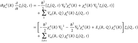5.40

The Q_n → Q_k = Q_n + ΔQ_nk transition, with n ≠ k, induces an ET event. PT also occurs if R_n and R_k = R_n + ΔR_nk are significantly different, namely, if the same ΔQ_nk triggers both ET and PT.

While the harmonic approximation and normal modes are used here (in particular, in eqs 5.39a and 5.39b, two terms with differently localized proton vibrational functions describe the proton state before and after a PT reaction), the interaction of the reactive proton with the Q modes is built into the total wave function in two ways: (a) χ_n^p belongs to the electronic state ϕ_n, and R_n = ⟨χ_n|R̂|χ_n^p⟩ arises from the potential field near the bottom of the nth basin; (b) the frequency of the normal mode associated with the motion of the proton and the related amplitude (e.g., as measured by the rms deviation from the mean value R_n of the proton position operator R̂(121)) depend on the interaction of the reactive proton with all nuclei. In fact, the vibrational frequency of the proton mode is obtained by diagonalizing the potential energy of interaction of all nuclei.²¹⁸ Thus, for a transition between two PFES basins characterized by ΔQ_nk and the related change in electronic charge localization (both expressed by a transition between two different terms of Ψ in eqs 5.39a and 5.39b), the properties of the whole system determine how the change ΔR_nk in the proton coordinate compares with the uncertainties δR_n = (⟨χ_n|R̂²|χ_n^p⟩ – ⟨χ_n|R̂|χ_n^p⟩²)^1/2 and δR_k of the proton position in its initial and final quantum states, namely, whether the localizations of the initial and final proton wave functions are sufficiently different to correspond to a PT process or not.

Equations 5.39a and 5.39b can be used to establish a more general PCET framework by also including wave functions ϕ_nχ_n^pχ_n and ϕ_kχ_kχ_k (with n ≠ k) such that χ_n^p and χ_k describe different proton localizations and are thus connected by a PT reaction, while ϕ_n and ϕ_k do not describe well-separated spatial distributions of the electron charge (i.e., ET), but rather differ by the electronic charge rearrangement that would accompany the PT. That is, one can use the same expression for Ψ to describe situations where ΔQ_nk causes ΔR_nk > δR_n, δR_k, namely, PT, and not ET. However, since PT occurs over short distances and the electronic coupling at short distances is usually large, the PT is electronically adiabatic. While, in principle, the diabatic wave functions ϕ_n and ϕ_k can still be used as electronic basis functions in the description of the PT reaction, it is useful to obtain an adiabatic subset of electronic wave functions by rotation of ϕ_n and ϕ_k and to use the adiabatic subset in the expression of the total wave function. If PT occurs with the electron in the adiabatic ground state, here denoted |ϕ_nk^ad⟩ (the subscripts indicate that this is the adiabatic ground state in a two-state model limited to ϕ_n and ϕ_k), it is sufficient to replace ϕ_n and ϕ_k by ϕ_nk in eqs 5.39a and 5.39b. For this pure PT event, accompanied by adiabatic rearrangement of electronic charge, ϕ_nk^ad corresponds to a single diabatic state with respect to ET. That is, the reaction occurs in a single basin of a landscape such as that shown in Figure 18b. ϕ_nk is present in one or two terms of Ψ depending on the vibrationally adiabatic/nonadiabatic nature of PT (see Figures 21 and 22). For vibrationally adiabatic PT, the proton wave functions χ_n^p and χ_k are obtained by application of a second BO adiabatic approximation to the R–Q subsystem (see section 5.2), and only one of them (which amounts to one term in Ψ) is involved in the electronically and vibrationally adiabatic PT reaction. The proton wave functions χ_n^p and χ_k are delocalized between R_n and R_k as shown in Figure 22b, but their amplitudes have a single maximum (at R_n ≅ R_n) in the limiting case of extremely strong interaction between the proton donor and acceptor (see Figure 21b), as would be expected for hydrogen bonds shorter than ∼2.5 Å. In this case, it is not meaningful to speak of PT, because the proton is delocalized between its donor and acceptor,²¹⁹ and again, a fortiori, a single term, ϕ_nχ_n^pχ_n, appears in the expansion of Ψ. For vibrationally nonadiabatic PT, χ_n and χ_k^p are localized wave functions, as in Figure 22a, and are obtained from linear combinations of the adiabatic vibrational functions. Two terms appear in the expansion of Ψ in eqs 5.39a and 5.39b to describe this electronically adiabatic and vibrationally nonadiabatic PT event. Note that Figures 21 and 22a,b represent slices, along the R coordinate and at Q_t, through an effective potential energy landscape of the kind shown in Figure 18.

Figure 22.

(a) Diabatic PESs for the initial and final ET states and vibrational wave functions φ_D^(I) (blue) and φ_A (red; notice that II = F in the notation of this review) for the phenoxyl–phenol system. The reaction is electronically nonadiabatic (see also section 12), so the vibronic coupling is the product of the electronic coupling and ⟨φ_D^(I)|φ_A⟩. (b) Adiabatic ground-state PES and pertinent proton vibrational functions for the benzyl–toluene system. The reaction is electronically adiabatic, and thus the vibronic coupling is half the splitting between the energies of the symmetric (cyan) and antisymmetric (magenta) vibrational states of the proton. The excited proton vibrational state is shifted up by 0.8 kcal/mol for a better visualization. Panels a and b reprinted from ref (197). Copyright 2006 American Chemical Society. (c) Two-dimensional diabatic electron–proton free energy surfaces for a PCET reaction connecting the vibronic states μ and ν as functions of two collective solvent coordinates: one strictly related to the occurrence of ET (z_e) and the other one associated with PT (z_p). The equilibrium coordinates in the initial and final states are marked, and the reaction free energy ΔG_μν° and reorganization energy λ_μν are indicated. Panel c reprinted from ref (221). Copyright 2006 American Chemical Society. (d) Free energy profile along the reaction coordinate represented by the dashed line in the nuclear coordinate plane of panel c. Qualitative proton PESs and pertinent ground-state proton vibrational functions are shown in correspondence to the reactant minimum, transition state, and product minimum. Panel d reprinted from ref (215). Copyright 2008 American Chemical Society.

The electron–proton wave functions (ϕ_nχ_n^p) can, in principle, be obtained by applying the BO approximation to separate the Schrödinger equations for the {q,R} and Q coordinates, without invoking a further BO approximation to describe the evolution of the q and R coordinates. The nonadiabatic couplings between the R and Q dynamics are in fact included by Hammes-Schiffer and co-workers (see below and section 12), thus obtaining a more accurate representation of the electron–proton wave functions involved in a PCET reaction and of the corresponding free energy surfaces (or electron–proton terms; see Figure 22c).^194,220

For PCET reactions with electronically nonadiabatic ET and electronically adiabatic PT, two sets of diabatic electronic states are sufficient to describe the overall PCET reaction mechanism (the two diabatic electronic states and the proton in the various possible vibrational levels).¹⁹⁴

The electron–proton PFESs shown in Figure 22c,d, which are obtained from the prescription by Hammes-Schiffer and co-workers,^214,221 are functions of two solvent (or, more generally, nuclear collective) coordinates, denoted z_e and z_p in Figure 22c. In fact, two different collective solvent coordinates describe the nuclear bath effects on ET and PT according to the PCET theory by Hammes-Schiffer and co-workers.^191,194,214 The PFES profile in Figure 22d is obtained along the reaction path connecting the minima of the two paraboloids in Figure 22c. This path represents the trajectory of the solvent coordinates for a classical description of the nuclear environment, but it is only the most probable reaction path among a family of quantum trajectories that would emerge from a stochastic interpretation of the quantum mechanical dynamics described in eq 5.40.

Insights into different effective potential energy surfaces and profiles such as those illustrated in Figures 21 and 22 and the connections among such profiles are obtained from further analysis of eqs 5.39 and 5.40. Understanding of the physical meaning of these equations is also gained by using a density matrix approach and by comparing orthogonal and nonorthogonal electronic diabatic representations (see Appendix B). Here, we continue the analysis in terms of the orthogonal electronic diabatic states underlying eq 5.40 and in the full quantum mechanical perspective. The discussion is formulated in terms of PESs, but the analysis in Appendix A can be used for interpretation in terms of effective PESs or PFESs.

Averaging eq 5.40 over the proton state for each n leads to a description of how the system dynamics depends on the Q mode, i.e., ultimately, on the probability densities that are associated with the different possible states of the reactive solvent mode Q:

5.41a

In this time-dependent Schrödinger equation, the explicit dependence of the electron transfer matrix element on nuclear coordinates is neglected (Condon approximation¹⁵⁹), S_nk^p = ⟨χ_n|χ_k^p⟩, and the electron–proton term E̅_n(Q) (namely, the Q-dependent average energy of the reactive electron–proton subsystem) is

5.41b

where

5.41c

is the average kinetic energy in state χ_n^p(R). The electron–proton terms are the PESs for the calculation of the nuclear wave functions χ_n sufficiently far from avoided crossings, where χ_n is indistinguishable from the vibrational wave function χ_n that satisfies the time-independent Schrödinger equation

5.42

which can also be obtained from a double-adiabatic approximation without the assumption that proton and other nuclear potentials are harmonic (see also section 9).

In the vibronically nonadiabatic regime, transitions among electron–proton states are determined by their vibronic couplings, which, in the PCET context, are defined¹⁹⁷ as the Hamiltonian matrix elements between reactant and product electron–proton vibrational wave functions. In the electronically nonadiabatic regime, with the Condon approximation, the vibronic coupling between two electron–proton diabatic states is well approximated by the product of the electronic coupling and the proton Franck–Condon factor. In biological systems, the nonadiabatic nature of an ET transition with small electronic coupling V_nk is, often, a consequence of distant and thus weakly interacting electron donors and acceptors with a large tunneling barrier protein intervening. Regarding the proton, instead, the large proton mass makes long-distance proton tunneling improbable. In fact, hydride and hydrogen atom transfers typically occur over distances of less than 3 Å, and often ET and PT involve different donor and acceptor groups.

When the same solvent coordinate Q couples to both electron and proton transitions, the nonadiabatic character of ET causes electronically nonadiabatic PT and, overall, vibronically nonadiabatic electron–proton transfer. This is because the nonadiabatic regime of ET implies (a) absence of correlation, in eq 5.41, between the vibrational functions χ_n that belong to different electronic states sufficiently far from the intersections among electron–proton PESs and (b) small transition probabilities near these intersections that are determined by the small values of the vibronic couplings. This means that the motion along the solvent coordinate is not limited to the ground-state vibronic adiabatic surface of Figure 23b. While eq 5.40 allows one to speak of (electronically) nonadiabatic ET, the combined effect of V_nk and S_nk^p on the couplings of eq 5.41 does not allow one to define a “nonadiabatic” or “vibrationally nonadiabatic” PT. This is in contrast with the case of pure PT between localized proton vibrational states along the Q coordinate. Hence, one can only speak of vibronically nonadiabatic EPT: this is appropriate when electronically nonadiabatic PT takes place,¹⁸² because the nonadiabaticity of the electronic dynamics coupled with PT implies the presence of the electronic coupling V_nk in the transition matrix element.

5.3.2. Investigating Coupled Electronic–Nuclear Dynamics and Deviations from the Adiabatic Approximation in PCET Systems via a Simple Model

Adiabatic electron–proton PESs are also shown in Figure 23b. To construct mixed electron/proton vibrational adiabatic states, we reconsider the form of eq 5.30 (or eq 5.32) and its solution in terms of adiabatic electronic states and the corresponding vibrational functions. To simplify the notation, and with focus on the reactive electron–proton subsystem, x denotes the overall set of nuclear coordinates {R,Q} or a reaction coordinate obtained as a linear combination of R and Q (or only R where the coupling of the electron and proton dynamics is examined without including Q effects). Given a complete set of electronic diabatic wave functions (ideally, an infinite set of strictly diabatic wave functions¹²⁸), diagonalization of the electronic Hamiltonian H at each value of x gives adiabatic electronic states that are solutions of

5.43

Equation 5.43 is the Schrödinger equation for the (reactive) electron at fixed nuclear coordinates within the BO scheme. Therefore, ϕ_α^ad is the electronic component of a BO product wave function that approximates an eigenfunction of the total Hamiltonian at x values for which the BO adiabatic approximation is valid. In fact, these adiabatic states give V_αβ = E_αδ_αβ, but correspond to (approximate) diagonalization of the full Hamiltonian (eq 5.1) only for small nonadiabatic kinetic coupling terms. We now (i) analyze and quantify, for the simple model in Figure 24, features of the nonadiabatic coupling between electronic states induced by the nuclear motion that are important for understanding PCET (therefore, the nonadiabatic coupling terms neglected in the BO approximation will be evaluated in the analysis) and (ii) show how mixed electron–proton states of interest in coupled ET–PT reactions are derived from the analysis of point i.

Figure 24.

(a) Typical (free) energy profile for ET or PCET along a reaction coordinate x (see the main text) and (b) its magnification near the transition-state coordinate (origin of the abscissa), using the diabatic energy difference Δ₁₂(x) as the reaction coordinate.^121,216,222 Both diabatic (dashed lines) and adiabatic (solid lines) curves are illustrated. Panel a qualitatively represents a case of electronically adiabatic reaction under the two-state approximation. However, the diabatic states ϕ₁ and ϕ₂ can still be used as a basis, and their connection with the electronic adiabatic states ϕ₁₂^ad and ϕ̃₁₂ is summarized in the inset, where H₀ is the channel Hamiltonian and V is a constant (Condon approximation) interaction component of the Hamiltonian. The dependence of H₀ on x can be formulated in terms of Δ₁₂. ϕ₁₂^ad and ϕ̃₁₂ are eigenfunctions of the electronic Hamiltonian for each Δ₁₂.

If we assume (as in eq 5.7) that the BO product wave function ϕ_α^ad(x,q) φ_α(x) (where φ_α(x) is the vibrational component) is an approximation of an eigenfunction of the total Hamiltonian , we have

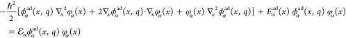5.44

Then, averaging over the electronic state, using the identity d_αα = 0 and eq 5.31, we find

5.45

with (via eq 5.21)

5.46

G_α^ad(x) + E_α(x) is an ‘”effective potential” for nuclear motion and contains the distortion of the electronic wave function due to its coupling to nuclear motion. The off-diagonal electronic–nuclear interaction terms of eq 5.44 are removed in eq 5.45 by averaging over a single electronic adiabatic state. However, these terms couple different adiabatic states. In fact, the scalar multiplication of eq 5.44 on the left by a different electronic adiabatic state, ϕ_β^ad, shows that the condition

5.47

must be satisfied for any α and β so that the BO adiabatic states are eigenfunctions of the full Hamiltonian and are thus solutions of eq 5.44. Indeed, eq 5.47 is generally not satisfied exactly even for two-state models. This is seen by using the equations in the inset of Figure 24 with the strictly electronic diabatic states ϕ₁ and ϕ₂. In this simple one-dimensional model, eqs 5.18 and 5.31 lead to the nuclear kinetic nonadiabatic coupling terms

5.48

and

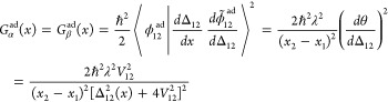5.49

It is easily seen that substitution of eqs 5.48 and 5.49 into eq 5.47 does not lead to a physically meaningful (i.e., appropriately localized and normalized) solution of eq 5.47 for the present model, unless the nonadiabatic coupling vector and the nonadiabatic coupling (or mixing¹²⁶) term determined by the nuclear kinetic energy (G_α^ad) in eq 5.47 are zero. Equations 5.48 and 5.49 show that the two nonadiabatic coupling terms tend to zero with increasing distance of the nuclear coordinate from its transition-state value (where Δ₁₂ = 0), thus leading to the expected adiabatic behavior sufficiently far from the avoided crossing. Considering that the nonadiabatic coupling vector is a Lorentzian function of the electronic coupling with width 2V₁₂, the extension (in terms of x or Δ₁₂, which depends linearly on x due to the parabolic approximation for the PESs) of the region with significant nuclear kinetic nonadiabatic coupling between the BO states decreases with the magnitude of the electronic coupling. Since the interaction V (see the Hamiltonian model in the inset of Figure 24) was not treated perturbatively in the above analysis, the model can also be used to see that, for sufficiently large V₁₂, a BO wave function behaves adiabatically also around the transition-state coordinate x_t, thus becoming a good approximation for an eigenfunction of the full Hamiltonian for all values of the nuclear coordinates.

Often, the validity of the adiabatic approximation is asserted on the basis of the comparison between the minimum adiabatic energy gap at x = x_t (that is, 2V₁₂ in the present model) and the thermal energy (namely, k_BT = 26 meV at room temperature). Here, instead, we analyze the adiabatic approximation taking a more general perspective (although the thermal energy remains a useful unit of measurement; see the discussion below). That is, we inspect the magnitudes of the nuclear kinetic nonadiabatic coupling terms (eqs 5.48 and 5.49) that can lead to the failure of the adiabatic approximation near an avoided crossing, and we compare these terms with relevant features of the BO adiabatic PESs (in particular, the minimum adiabatic splitting value). Since, as said above, the reaction nuclear coordinate x is the coordinate of the transferring proton, or closely involves this coordinate, our perspective emphasizes the interaction between electron and proton dynamics, which is of special interest to the PCET framework.

Consider first that, at the transition-state coordinate x_t, the nonadiabatic coupling (in eV) determined by the nuclear kinetic energy operator (eq 5.49) is

5.50

where x is a mass-weighted coordinate (hence, it is proportional to the square root mass associated with the reactive nuclear mode) and the dimensionless quantity f is the magnitude of the effective displacement of the relevant nuclear coordinate x expressed in angstroms. Since we are investigating the conditions for electronic adiabaticity, the PESs in Figure 24 may represent the electronic charge distributions in the initial and final proton states of a pure PT reaction or different localizations of a reactive electron for HAT or EPT with short-distance ET. Thus, we can take f in the range of 0.5–3 Å, which leads to values of the numerical factor in the last expression of eq 5.50 in the range of 6 × 10^–5 to 2 × 10^–3. For example, for f = 1 and λ = 0.25 eV, an electronic coupling V₁₂ ≈ 0.06 eV ≈ 5k_BT/2 is large enough to make G_α^ad(x_t) ≈ 0.01 eV, i.e., less than k_BT/2. Indeed, for the x displacement considered, the coupling is usually larger than 0.06 eV. Thus, in conclusion, the minimum adiabatic energy splitting cannot be overcome by thermal fluctuation, on the one hand, and is not appreciably modified by G_α, on the other hand.

To evaluate the effect of the nonadiabatic coupling vector on the PES landscape, either in the semiclassical picture of eq 5.24 or in the present quantum mechanical picture, one needs to compute

5.51

where x is a mass-weighted proton coordinate and ẋ is a velocity associated with x. Indeed, in this simple model one may consider the proton as the “relative particle” of the proton–solvent subsystem whose reduced mass is nearly identical to the mass of the proton, while the whole subsystem determines the reorganization energy.

We need to consider a model for ẋ to evaluate the expression in eq 5.51, and hence to investigate the relation between the value of V₁₂ and that of the nonadiabatic coupling in eq 5.51. This relationship will be studied throughout the regime of proton tunneling (i.e., for values of V₁₂ such that the proton vibrational levels are lower than the potential energy barrier in Figure 24).

As in ref (195), we define a proton “tunneling velocity” ẋ as it appears in Bohm’s interpretation of quantum mechanics,²²³ namely, by using appropriate parameters for the present model:

5.52

In eq 5.52, the proton energy is approximated by its ground-state value in one of the parabolic diabatic potentials of Figure 24a, and distortions of the potential at its minimum by V₁₂ are neglected. Using the equations in the inset of Figure 24 and expressing both ℏω_p and λ in electronvolts, we obtain

5.53

Equation 5.53 gives ℏω_p ≈ 0.05 eV, so ω_p ≈ 0.7 × 10¹⁴ s^–1, for the chosen values of f and λ. The other parameter (E_act) in the expression of ẋ is the activation energy. From the energy of the lower adiabatic state

5.54

(note that E_β^ad differs from E_α by the sign of the square root), one obtains the energy barrier

5.55

Insertion of eqs 5.52–5.55 into eq 5.51 gives

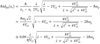5.56

The numerical factor 0.09/4f in the last line of eq 5.56 is used with electronic couplings and reorganization energies in electronvolts. The value of the nonadiabatic term in eq 5.56 is ≤0.01 eV when V₁₂ ≳ 0.05 eV, which is a condition well satisfied for distances on the order of 1 Å. Therefore, the minimum PES splitting is significantly larger than ℏẋd_βα(x_t), and the effect of this nonadiabatic coupling on the PES landscape of Figure 24 can be neglected, which means that the BO adiabatic states are good approximations to the eigenstates of the Hamiltonian .

The present analysis of ℏẋd_βα and G_α^ad clarifies and quantifies the electronically adiabatic nature of PT when the relevant nuclear coordinate for the combined ET–PT reaction is the proton displacement and is on the order of 1 Å. For a pure ET reaction (also see the useful comparison, in the context of ET, of the electronic and nonadiabatic couplings in ref (127)), x in Figure 24 may be a nuclear reaction coordinate characterized by larger displacements (and thus larger f values) than the proton coordinate in electron–proton transfer, but the relevant modes usually have much smaller frequencies (e.g., ω ≈ 10¹¹ s^–1; see section 9) than proton vibrational frequencies. Consequently, according to eq 5.56, the electronic coupling threshold for negligible ℏẋd_βα(x_t) values (i.e., for the onset of the adiabatic regime) can be much smaller than the 0.05 eV value estimated above. However, the V₁₂ value decreases approximately exponentially with the ET distance, and the above analysis applied to typical biological ET systems leads to the nonadiabatic regime. In general, charge transfer distances, specifics of charge localization and orientation, coupled PT, and relevant nuclear modes will determine the electronic diabatic or adiabatic nature of the charge transfer. The above discussion offers insight into the physics and the approximations underlying the model system used by Georgievskii and Stuchebrukhov¹⁹⁵ to describe EPT reactions, but it also provides a unified framework to describe different charge transfer reactions (ET, PT, and EPT or the special case of HAT). The following points that emerge from the above discussion are relevant to describing and understanding PES landscapes associated with ET, PT, and EPT reactions:

(i) Smaller V₁₂ values produce a larger range of the proton–solvent conformations on each side of the intersection between the diabatic PESs where the nonadiabatic couplings are negligible. This circumstance leads to a prolonged adiabatic evolution of the charge transfer system over each diabatic PES, where V₁₂/Δ₁₂ is negligible (e.g., see eq 5.54). However, smaller V₁₂ values also produce stronger nonadiabatic effects close enough to the transition-state coordinate, where 2V₁₂ becomes significantly larger than the diabatic energy difference Δ₁₂ and eqs 5.50 and 5.51 apply.

(ii) The minimum energy separation between the two adiabatic surfaces increases with V₁₂, and the effects of the nonadiabatic couplings decrease. This means that the two BO states become good approximations of the exact Hamiltonian eigenstates. Instead, as shown by eq 5.54, the BO electronic states can differ appreciably from the diabatic states even near the PES minima when V₁₂ is sufficiently large to ensure electronic adiabaticity across the reaction coordinate range.

(iii) This simple two-state model also predicts increasing adiabatic behavior as V₁₂/λ grows, i.e., as the adiabatic splitting increases and the energy barrier (∼λ/4) decreases. Even if V₁₂ ≫ k_BT, so that the model leads to adiabatic ET, the diabatic representation may still be convenient to use (e.g., to compute energy barriers) as long as the electronic coupling is much less than the reorganization energy.

5.3.3. Formulation and Representations of Electron–Proton States

The above analysis sets conditions for the adiabaticity of the electronic component of BO wave functions. Now, we distinguish between the proton coordinate R and another collective nuclear coordinate Q coupled to PCET and construct mixed electron/proton vibrational adiabatic states with a double-adiabatic separation scheme. Thus, either the PT or the ET time scale—or both—can cause nonadiabaticity of the electron–proton states. Using eqs 5.44 and 5.45, a procedure to obtain electron–proton wave functions and PESs (typical ones are shown in Figure 23b) is as follows:

(i) The electronic Hamiltonian is diagonalized at every {R,Q} (typically, on a 2D grid in the R, Q plane) to obtain a basis of adiabatic electronic states. This can be done beginning with a diabatic set, when it is available, thus providing the electronic part of

5.57

that satisfies

5.58

at each fixed point {R,Q}, and the corresponding energy eigenvalue.

(ii) Substitution into the Schrödinger equation Ψ_α^ad = Ψ_α, where = T̂_{R,Q} + H, and averaging over the electronic state lead to

5.59

where

5.60

and E_α^ad(R,Q) are known from point i.

(iii) If the kth and nth diabatic states are involved in the PCET reaction (see Figure 23), the effective potential E_α^ad(R,Q) + G_αα(R,Q) for the motion of the proton–solvent system is characterized by potential wells centered at R_k and R_n along the R coordinate and at Q_k and Q_n along Q. Then analytical solutions of eq 5.59 of the form

5.61

are possible, for example, by approximating the effective potential as a double harmonic oscillator in the R and Q coordinates.²²⁴

(iv) Substitution of eq 5.61 into eq 5.59 and averaging over the proton state yield

5.62a

where

5.62b

and

5.62c

with

5.62d

Hence, E̅_α^p,ad(Q) + G̅_αα(Q) is the electron–proton term. This term is the “effective potential” for the solvent-state dynamics, but it includes, in G̅_αα^p,ad, the distortion of the electronic wave function due to its coupling with the same solvent dynamics. In turn, the effect of the Q motion on the electronic wave functions is reflected in the corresponding proton vibrational functions. Therefore, interdependence between the reactive electron–proton subsystem and the solvent is embodied in eqs 5.62a–5.62d. Indeed, an infinite number of electron–proton states result from each electronic state and the pertinent manifold of proton vibration states.

The distance from an avoided crossing that causes ϕ_α^ad to become indistinguishable from ϕ_k or ϕ_n (in the case of nonadiabatic charge transitions) was characterized in eq 5.48 using the Lorentzian form of the nonadiabatic coupling vector d_βα. Equation 5.48 shows that the value of d_βα depends on the relative magnitudes of the energy difference between the diabatic states (chosen as the reaction coordinate¹²¹) and the electronic coupling. The fact that the ratio between V_kn and the diabatic energy difference measures proximity to the nonadiabatic regime¹⁴⁴ can also be established from the rotation angle θ (see the inset in Figure 24) connecting diabatic and adiabatic basis sets as a function of the R and Q coordinates. From the expression for the electronic adiabatic ground state ϕ_kn, we see that ϕ_kn^ad ≅ ϕ_n if V_kn/Δ_kn ≪ 1 (θ ≅ 0; E_k > E_n) or ϕ_kn ≅ ϕ_k if −V_kn/Δ_kn ≪ 1 (θ ≅ 0; E_k < E_n). Thus, for sufficiently small V_kn, one can use the piecewise approximation

5.63

and eq 5.42 is valid within each diabatic energy range. Equation 5.63 provides a simple, consistent conversion between the diabatic and adiabatic pictures of ET in the nonadiabatic limit, where the small electronic couplings between the diabatic electronic states cause decoupling of the different states of the proton–solvent subsystem in eq 5.40 and of the Q mode in eq 5.41a. However, while small V_kn values represent a sufficient condition for vibronically nonadiabatic behavior (i.e., ultimately, V_knS_kn^p ≪ k_BT), the small overlap between reactant and product proton vibrational wave functions is often the cause of this behavior in the time evolution of eq 5.41.²¹⁵ In fact, the distance dependence of the vibronic couplings V_knS_kn is determined by the overlaps S_kn^p.^197,225

Detailed discussion of analytical and computational approaches to obtain mixed electron/proton vibrational adiabatic states is found in the literature.^214,226,227 Here we note that the dimensional reduction from the {R,Q} to the {Q} conformational space in going from eq 5.40 to eq 5.41 (or from eq 5.59 to eq 5.62) does not imply a double-adiabatic approximation or the selection of a reaction path in the R, Q plane. In fact, the above procedure treats R and Q on an equal footing up to the solution of eq 5.59 (such as, e.g., in eq 5.61). Then, eq 5.62 arises from averaging eq 5.59 over the proton quantum state (i.e., overall, over the electron–proton state for which eq 5.40 expresses the rate of population change), so that only the solvent degree of freedom remains described in terms of a probability density. However, while this averaging does not mean application of the double-adiabatic approximation in the general context of eqs 5.40 and 5.41, it leads to the same result where the separation of the R and Q variables is allowed by the harmonic and Condon approximations (see, e.g., section 9 and ref (180)), as in eqs 5.59−5.62.

Within the standard adiabatic approximation, the effective potential E_n(R,Q) in eq 5.40 or E_α^ad(R,Q) + G_αα(R,Q) in eq 5.59 provides the effective potential energy for the proton motion (along the R axis) at any given solvent conformation Q, as exemplified in Figure 23a. Comparing parts a and b of Figure 23 provides a link between the behavior of the system around the diabatic crossing of Figure 23b and the overlap of the localized reactant and product proton vibrational states, since the latter is determined by the dominant range of distances between the proton donor and acceptor allowed by the effective potential in Figure 23a (let us note that Figure 23a is a profile of a PES landscape such as that in Figure 18, orthogonal to the Q axis). This comparison is similar in spirit to that in Figure 19 for ET,⁷ but it also presents some important differences that merit further discussion.

In the diabatic representation or the diabatic approximation of eq 5.63, the electron–proton terms in Figure 23b cross at Q = Q_t, where the potential energy for the motion of the solvent is E̅_n^p(Q_t) and the localization of the reactive subsystem in the kth or nth potential well of Figure 23a corresponds to the same energy. In fact, the potential energy of each well is given by the average electronic energy E_j(R,Q_t) = ⟨ϕ_j(R,Q_t)|V(R̂,Q_t,q̂) + T̂_q|ϕ_j(R,Q_t)⟩ (j = k, n), and the proton vibrational energies in both wells are ⟨χ_j|E_j(R,Q_t)|χ_j^p⟩ + T_j = E̅_j^p(Q_t).

In reference to the electronically adiabatic surfaces in Figure 23b, their splitting at Q_t is not neglected, and eqs 5.62a–5.62d are thus used. The minimum splitting is E̅_β^p,ad(Q_t) – E̅_α(Q_t) + G̅_ββ^p,ad(Q_t) − G̅_αα(Q_t), where the derivatives with respect to Q in the diagonal interaction terms G̅_αα^p,ad(Q_t) and G̅_ββ(Q_t) are taken at Q = Q_t and β marks the upper adiabatic electronic state and the corresponding electron–proton energy eigenvalue. G̅_ββ^p,ad(Q_t) – G̅_αα(Q_t) is zero for a model such as that shown in Figure 24 with θ(R,Q). Thus, averaging E_α^ad(R,Q) – ℏ²∇_R²/2 and E_β(R,Q) – ℏ²∇_R²/2 over the respective proton wave functions gives

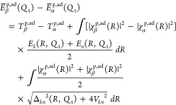5.64

If pure ET occurs, χ_β^p,ad(R) = χ_α(R). Thus, T_β^p,ad = T_α and the minima of the PFESs in Figure 18a (assumed to be approximately elliptic paraboloids) lie at the same R coordinate. As such, the locus of PFES intersection, Δ_kn(R,Q_t) = 0, is perpendicular to the Q axis and occurs for Q = Q_t. Thus, eq 5.64 reduces to

5.65

(where the Condon approximation with respect to R was used).

Figure 23c is obtained at the solvent coordinate Q̅, for which the adiabatic lower and upper curves are each indistinguishable from a diabatic curve in one PES basin. In this case, E_k(R,Q̅) and E_n(R,Q̅) are the left and right potential wells for proton motion, and E̅_β^p,ad(Q̅) – E̅_α(Q̅) ≅ E̅_k^p(Q̅) – E̅_n(Q̅). Note that E̅_β^p,ad(Q) – E̅_α(Q) is the energy difference between the electron–proton terms at every Q, including the transition-state region, for electronically adiabatic ET (and hence also for PT, as discussed in section 5.2), where the nonadiabatic coupling terms are negligible and thus only the lower adiabatic surface in Figure 23, or the upper one following excitation, is at play.

The diabatic electron–proton terms in Figure 23b have been related, in the above analysis, to the proton vibrational levels in the electronic effective potential for the nuclear motion of Figure 23a. Compared to the case of pure ET in Figure 19, the focus in Figure 23a is on the proton coordinate R after averaging over the (reactive) electronic degree of freedom. However, this parallelism cannot be extended to the relation between the minimum adiabatic PES gap and the level splitting. In fact, PT takes place between the χ_k^p,ad(R) and χ_n(R) proton vibrational states that are localized in the two wells of Figure 23a (i.e., the localized vibrational functions φ_D^(I) and φ_A in the notation of Figure 22a), but these are not the proton states involved in the adiabatic electron–proton PESs of Figure 23b. The latter are, instead, χ_α^p,ad, which is the vibrational component of the ground-state adiabatic electron–proton wave function ϕ_α(R,Q,q)χ_α^p,ad(R) and is similar to the lower-energy linear combination of χ_k and χ_n^p,ad shown in Figure 22b, and χ_β, which is the lowest vibrational function belonging to the upper adiabatic electronic wave function ϕ_β^ad.

Two electron–proton terms with the same electronic state, ϕ_α^ad(R,Q,q) χ_α(R) and ϕ_α^ad(R,Q,q) χ_α(R) (here, p is also the quantum number for the proton vibration; p₁ and p₂ are oscillator quantum numbers), can be exploited to represent nonadiabatic ET in the limit V_kn → 0 (where eq 5.63 is valid). In fact, in this limit, the PES corresponding to ϕ_α^ad is indistinguishable from the diabatic PESs near their minima, and the minimum of the diabatic crossing seam is a good approximation to the activation barrier (however, V_kn is never exactly zero if ET can occur, and the computation of this coupling requires knowledge of the excited adiabatic state or of the corresponding diabatic states). In addition, linear combinations of χ_α and χ_α^p₂,ad yield the localized proton wave functions for the electronic diabatic states. More generally, ϕ_α(R,Q,q) χ_α^p₁,ad(R) and ϕ_α(R,Q,q) χ_α^p₂,ad(R) can be used to describe electronically adiabatic PCET reactions. One of these functions suffices to describe the vibrationally adiabatic PT, while both are necessary to describe vibrationally nonadiabatic PT in the adiabatic (proton vibrational) representation. Thus, in the electronically adiabatic case, the full analogue of Figure 19 is regained and the vibronic coupling is half the splitting between the two vibrational state energies, so that Figure 22a is the analogue of Figure 19a after averaging over the quantum state of the electron and with reference to the proton motion. In particular, PT on an electronically adiabatic surface, without involvement of ET, was treated in analogy with ET by Borgis and Hynes.²²⁸

While parts a and c of Figure 23 are obtained for specific solvent coordinates, averaging eq 5.40 over solvent quantum states leads to the R coordinate equations of motion that should be used in models that include only the electron and proton coordinates (e.g., in ref (195)):

5.66a

The Condon approximation was used to derive eq 5.66a, where S_nk = ⟨χ_n|χ_k⟩ and

5.66b

with

5.66c

Moreover, in analogy with eq 5.42, when the kinetic nonadiabatic coupling is negligible, χ_n^p(R) is nearly identical to the wave function χ_n(R) that satisfies the time-independent Schrödinger equation

5.67

The symmetry of eqs 5.41–5.42 and eqs 5.66–5.67 with respect to Q and R arises from the Condon approximation. In this approximation, V_nk does not depend appreciably on R and Q, so ⟨χ_n^p|V_nk|χ_k⟩ = V_nkS_nk^p and ⟨χ_n|V_nk|χ_k⟩ = V_nkS_nk. If the Condon approximation is invalid, the averages over the proton and solvent states correspond to qualitatively different vibronic couplings, because V_nk in general depends differently on R and Q.

The electronic adiabatic states arise from the analogue of eqs 5.62a–5.62d:

5.68a

where

5.68b

and

5.68c

with

5.68d

Equations 5.41a–5.41c show that, for nonadiabatic ET and coupling of PT and ET to the same displacement of the solvent mode, the PCET reaction mechanism is vibronically nonadiabatic. Equations 5.66 provides further information on the reaction mechanism, since it indicates the electronic nonadiabaticity of the PT. The ET and PT reactions may be induced by the same Q change also in cases where the two reactions involve different pathways (for example, a fluctuation brings the electron donor and acceptor close enough to enable ET, and the ET event triggers the coupled PT). However, in general, one expects that ET and PT are coupled to different changes in the nuclear coordinates. Thus, nonadiabatic ET can be coupled to adiabatic PT, which amounts to inserting electronic wave functions such as ϕ_nk^ad into the wave function expansion of eq 5.39a or eq 5.39b (see the discussion at the beginning of this subsection). The overall change in the nuclear environment corresponding to EPT can then be represented as indicated in Figure 18, while the same kind of representation may prove inadequate for PT/ET or ET/PT (see Figure 25a). In PT/ET, PT₁ and ET_b involve changes in Q in the same direction but of different magnitudes. For ET/PT, the change in Q that induces ET_a includes the Q displacement required for PT₁, but the PT takes place only after ET. This example emphasizes that, in general, the theoretical modeling of PCET reactions requires two different nuclear reaction coordinates for ET and PT, as described by Borgis and Hynes^165,192 or by Hammes-Schiffer and co-workers^191,194,214 (see Figure 25b). These strategies enabled “natural” treatments of situations where, even for vibronically nonadiabatic PCET, the PT process can be electronically nonadiabatic, electronically adiabatic, or intermediate.^{182,184,197,215} The above analysis also holds, indeed, in the presence of two Q modes (Q_e for ET and Q_p for PT).

Figure 25.

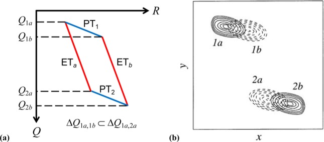
(a) Description of coupled PT and ET reactions using a single solvent coordinate Q. The Q values for the states in Figure 20 are indicated. If the reaction mechanism is ET/PT, the change in Q that induces the ET_a process (ΔQ_1a,2a) includes the Q displacement required for the occurrence of PT₁ (ΔQ_1a,1b), but PT occurs following ET. (b) The treatment of Soudackov and Hammes-Schiffer removes the inconsistency in panel a by introducing two different solvent coordinates, x and y, for PT and ET, respectively. Panel b reprinted with permission from ref (191). Copyright 2000 American Institute of Physics.

In the above analysis in terms of normal modes, S_nk^p and S_nk are vibrational function overlaps, independent of the coordinates, between quantum states for the R and Q modes. However, eqs 5.40, 5.41, and 5.66 entangle the R and Q dynamics, and thus the motions of the two degrees of freedom are correlated. If Q can be described classically, then a typical correlation between the R and Q motions is as follows: Q is an internal coordinate related to the positions, or relative position, of the charge donor and acceptor (e.g., see Figure 26), while |χ_k⟩ and |χ_n^p(Q)⟩ are quantum oscillator proton states, and the latter is centered at a position that depends on Q. In this semiclassical view, the overlap between the two proton states depends on Q, but this is consistent with the fully quantum mechanical view of eqs 5.40, 5.41, and 5.66, where the vibrational function overlaps are independent of the nuclear coordinates.

Figure 26.

Schematic of a PT event (coupled to an ET reaction) where Q_k is the initial nuclear coordinate (left), Q_t is the transition-state coordinate (center), Q_n is the final coordinate (right), and ΔQ_kn = Q_n – Q_k. The overlap of the proton wave functions is a maximum at Q_t.

The consistency of the two views is understood using the double-adiabatic approximation in a fully quantum description of the system. In this description, |χ_k^p⟩ is a proton vibrational state belonging to the kth electronic state. The Q mode is described by a wave packet. The |χ_n(Q)⟩ proton state is obtained by application of the double-adiabatic approximation and thus depends parametrically on Q. |χ_n^p(Q)⟩ is not, at all Q, the vibrational proton state |χ_n⟩ belonging to the nth electronic state when the latter is a strictly diabatic state computed at the equilibrium nuclear coordinate Q_n of the nth PES basin. The wave function that corresponds to the state vector |χ_n^p(Q)⟩ is χ_n(R,Q). That is, this proton wave function depends on R and parametrically on Q. In particular, its values along the trajectory ⟨Q(t)⟩ of the wave packet are χ_n^p(R,Q(t)).

This example highlights the value of the double-adiabatic approximation, where it can be applied, for a convenient description and interpretation of reaction mechanisms. If the two-state approximation holds with respect to the proton state, the motion of the system can also be represented in terms of |χ_k^p⟩ and |χ_n⟩, and clearly the coefficients of these proton states in the system state evolve differently compared to the case where |χ_n^p(Q)⟩ is used as one of the proton basis states.

As discussed above, free energy is generally represented as indicated in Figure 18. Q usually represents a set of classical degrees of freedom (e.g., the x and y coordinates in Figure 25). The Landau–Zener approach^154−157 and its extensions¹⁹⁵ can be used to describe the system behavior at avoided crossings.

The energy (or, as a result of thermal averaging, free energy) parameters of interest are included in eqs 5.40, 5.41, and 5.66, as they are determined by the coordinate dependencies of E_n(R,Q), E̅_n^p(Q), and E̅_n(R), respectively. The reorganization (free) energy and the reaction free energy play a crucial role in determining the PCET mechanism, and the familiar relationship between the activation energy and these two parameters^147,148,158 in the Marcus ET theory remains essentially valid in all PCET rate expressions. In a multistate picture, each state is characterized by specific values of the two free energy parameters that account for the special role of the transferring proton as compared to the other nuclear degrees of freedom¹⁸⁴ (see below).

The PCET mechanism that takes place in a given system and, in particular, the number of electron–proton distinguishable states in the reaction depend critically on the relative heights of the activation barriers for the charge transfer processes at play. For example, in ref (229), the Marcus theory analysis of self-exchange reactions between high-spin iron 2,2′-biimidazoline complexes shows that the free energy barriers for the ET_a and PT₁ processes (Figure 20) are much higher than for the concerted ET and PT. Thus, concerted ET and PT is the reaction mechanism, rather than the sequential charge transfer 1a → 2a → 2b or 1a → 1b → 2b.

This kind of analysis also emerges from representations of the involved electronic states as functions of the proton coordinate, such as in Figure 27, reported from ref (215). As described in our analysis, although pure PT is expected to be electronically adiabatic, one can still represent the related electronic charge distributions using diabatic electronic wave functions: this is also done in Figure 27a,b (blue curves) for the 1a → 1b and 2a → 2b proton transitions (see eq 5.38). Figure 27a shows the four diabatic states of eq 5.38 and Figure 20 and the adiabatic states obtained by diagonalizing the electronic Hamiltonian. The reactant (I) and product (II) electronic states corresponding to the ET reaction are adiabatic with respect to the PT process. These states are mixtures of states 1a, 1b and 2a, 2b, respectively, and are shown in Figure 27b,c. Their diagonalization would lead to the two lowest adiabatic states in Figure 27a. This figure corresponds to situations where the reactant (product) electronic charge distribution strongly favors proton binding to its donor (acceptor). In fact, the minimum of PES 1a (2b) for the proton in the reactant (product) electronic state is in the proximity of the proton donor (acceptor) position. In the reactant electronic state, the proton ground-state vibrational function is localized in 1a, with negligible effects of the higher energy PES 1b. A change in proton localization without concurrent ET leads to an energetically unfavorable electronic charge distribution (let us note that the 1a → 1b diabatic-state transition does not correspond to ET, but to electronic charge rearrangement that accompanies the PT reaction; see eq 5.38). Similar arguments hold for 2b and 2a in the product electronic state. These far proton localizations in the reactant and product electronic states lead to their small overlap and correspondingly small vibronic coupling. In other words, V₁₂S_1a,2b^p can even be significantly smaller than the thermal energy because of the small value of S_1a,2b. That is, PCET occurs in the vibronically nonadiabatic regime. For very large reaction free energies between 1a and 1b and between 2a and 2b, PESs I and II reduce to parabolas that describe EPT or HAT. Conversely, if the 1a (2a) and 1b (2b) minima are similar in energy, all diabatic states in eq 5.38 can be involved in the reaction mechanism. Applying the analysis of this section to the biochemical systems of Table 1, we predict the PCET regimes tabulated in the last two columns of the table.

Figure 27.

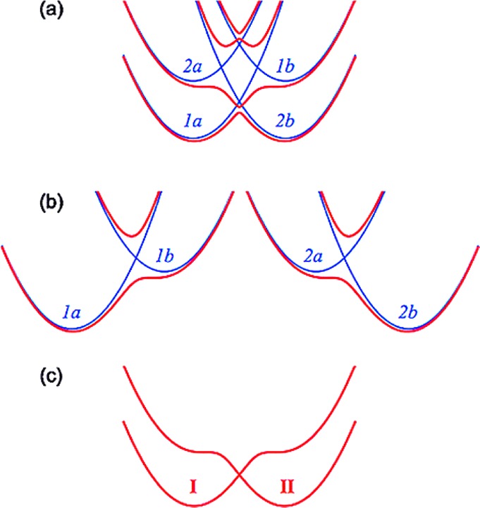
(a) Diabatic (1a, 1b, 2a, and 2b, in blue) and adiabatic (red) electronic states as functions of the proton coordinate, drawn for a reaction with nonadiabatic ET and electronically adiabatic PT. The adiabatic states are obtained by diagonalizing the 4 × 4 Hamiltonian matrix for the electron–proton subsystem (H_ep in section 12). (b) Neglecting the small electronic couplings between the 1a/2a and 1b/2b states, diagonalization of the 2 × 2 blocks corresponding to the 1a/1b and 2a/2b state pairs yields the electronic states represented by the red curves. (c) The two lower electronic states in panel b are reported. They are the initial and final diabatic ET states. Each of them is an adiabatic electronic state for the PT reaction. The numbers “1” and “2” correspond to I and F, respectively, in the notation of section 12.2. Reprinted from ref (215). Copyright 2008 American Chemical Society.

6. Extension of Marcus Theory to Proton and Atom Transfer Reactions

The analysis performed in section 5 emphasized the links among ET, PT, and PCET and made use of the Schrödinger equations and BO approach to provide a unified view of these charge transfer processes. The strong connections between ET and PT have provided a natural framework to develop many PT and PCET theories. In fact, Marcus extended his ET theory to describe heavy particle transfer reactions, and many deliberately generic features of this extension allow one to include emerging aspects of PCET theories. The application of Marcus’ extended theory to experimental interpretation is characterized by successes and limitations, especially where proton tunneling plays an important role. The analysis of the strong connections between this theory and recent PCET theories may suggest what complications introduced in the latter are critical to describe experiments that cannot be interpreted using the Marcus extended theory, thus leading to insights into the physical underpinnings of these experiments. This analysis may also help to characterize and classify PCET systems, enhancing the predictive power of the PCET theories. The Marcus extended theory of charge transfer is thus discussed here.

6.1. Extended Marcus Theory for Electron, Proton, and Atom Transfer Reactions

Early applications and extensions of Marcus theory to proton and atom transfer reactions were described by Sutin^230,231 and by Marcus.²³² In fact, Marcus’ analysis begins with the ET cross-relation in the weak-coupling limit.

Consider the self-exchange weak-overlap ET reactions

6.1

and the cross-reaction

6.2

By assuming the following approximation for the reorganization energy associated with the cross-reaction:^232,233

6.3

the rate constants k_nn (n = 1, 2) and k₁₂ for eqs 6.1 and 6.2 are related by

6.4

where

6.5

is the equilibrium constant for the ET cross-reaction. f₁₂ is often close to unity,⁷ and

6.6

Equations 6.4 and 6.6 hold for κ_el ≅ 1 and neglect the work terms associated with forming the precursor and successor complexes, except that their difference can be included in the reaction free energy ΔG_R° (see ref (7)). Indeed, the rate constants of the bimolecular reactions in solution need to be inserted into eq 6.4 for comparison to experiments. These rate constants include the work terms w^r and w^p that are required to bring the reactants and products to the mean charge donor–acceptor distance in the activated complex. In this perspective, the ET cross-reaction rate is^{7,122,233−235}

6.7

In eq 6.7, the energy ratio in the exponent is written on a per molecule basis, Z is a bimolecular collision frequency, and the activation free energy is

6.8a

with

6.8b

In eq 6.8b, ΔG° is the “standard” free energy of reaction^7,122,236 for separated reactants and products.^237,238

Assuming that Z is approximated well by the geometric mean of the homologous frequencies for the self-exchange reactions, Z₁₁ and Z₂₂, and that eq 6.3 holds, eqs 6.4 and 6.6 are replaced by²³⁹ (see also the Supporting Information)

6.9a

with

6.9b

and

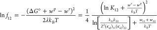6.10

In eq 6.10, w_nn = w_nn^r = w_nn (n = 1, 2) are the work terms for the exchange reactions. If (i) these terms are sufficiently small, or cancel, or are incorporated into the respective rate constants and (ii) if the electronic transmission coefficients are approximately unity, eqs 6.4 and 6.5 are recovered.

The cross-relation in eq 6.4 or eq 6.9 was conceived for outer-sphere ET reactions. However, following Sutin,²³⁰ (i) eq 6.4 can be applied to adiabatic reactions where the electronic coupling is sufficiently small to neglect the splitting between the adiabatic free energy surfaces in computing the activation free energy (in this regime, a given redox couple may be expected to behave in a similar manner for all ET reactions in which it is involved²³⁰) and (ii) eq 6.4 can be used to fit kinetic data for inner-sphere ET reactions with atom transfer.^230,231 These conclusions, taken together with encouraging predictions of Brønsted slopes for atom and proton transfer reactions,²⁴⁰ and cues from a bond energy–bond order (BEBO) model used to calculate the activation energies of gas-phase atom transfer reactions, led Marcus to develop extensions of eq 5.29 applicable to “strong-overlap” reactions such as atom and proton transfers and to strong-overlap ET.²³²

Extending the Marcus theory for ET between weakly interacting redox partners to proton and atom transfer reactions²³² requires reconsideration of the assumptions leading to the free energy factor in the Marcus rate expression. Mainly Coulombic work is performed to bring reactants together,²³³ but the main contribution to the free energy barrier for ET is provided by readjusting bond lengths and angles in the reactants (i.e., inner-sphere contributions) and by the reorientation of solvent molecules (outer-sphere contribution). The vibrational motion of the ligands and the dielectric relaxation of the solvent polarization through many degrees of freedom, in the linear response regime, lead to the parabolic PFESs that are described in Marcus’ ET theory and the related dependence of the activation barrier ΔG* for ET on the reorganization (free) energy λ and on the driving force (ΔG_R° or ΔG°). λ is the intrinsic (inner-sphere plus outer-sphere) activation barrier; namely, it is the kinetic barrier in the absence of a driving force.²²⁹ ΔG_R°, or ΔG°, represents the thermodynamic, or extrinsic,²³² contribution to the reaction barrier, which can be separated from the λ effect using the cross-relation of eq 6.4 or eq 6.9 and the concept of the Brønsted slope^232,241 (see below).

Proton and atom transfer reactions involve bond breaking and making, and hence degrees of freedom that essentially contribute to the intrinsic activation barrier. If most of the reorganization energy for these reactions arises from nuclear modes not involved in bond rupture or formation, eqs 6.6−6.8 are expected also to describe these reactions.²³² In this case, the nuclear degrees of freedom involved in bond rupture–formation give negligible contributions to the reaction coordinate (as defined, e.g., in refs (168) and (169)) along which PFESs are plotted in Marcus theory. However, in the many cases where the bond rupture and formation contribute appreciably to the reaction coordinate,²³² the potential (free) energy landscape of the reaction differs significantly from the typical one in the Marcus theory of charge transfer. A major difference between the two cases is easily understood for gas-phase atom transfer reactions:

6.11

Stretching one bond and compressing another leads to a potential energy that, as a function of the reaction coordinate, is initially a constant, experiences a maximum (similar to an Eckart potential²⁴²), and finally reaches a plateau.²³² This significant difference from the potential landscape of two parabolic wells can also arise for reactions in solution, thus leading to the absence of an inverted free energy effect.²⁴³ In these reactions, the Marcus expression for the adiabatic charge-transfer rate requires extension before application to proton and atom transfer reactions. This extension was described by Marcus, writing the activation energy for the gas-phase reaction as^240,244

6.12a

6.12b

6.12c

The potential energy difference ΔE° replaces the free energy ΔG_R° in gas-phase reactions, and λ̅ is a “reorganization property” of the system that satisfies, and is defined by, the additivity relationship

6.13

For atom transfer reactions in solution with a reaction coordinate dominated by bond rupture and formation, the analogue of eqs 6.12a–6.12c assumes the validity of the Marcus rate expression as used to describe adiabatic ET for |ΔG_R°| ≤ λ and imposes the condition of an exclusively extrinsic free energy barrier (i.e., λ = 0) outside of this range:²³²

6.14a

6.14b

Thus, the general treatment of proton and atom transfer reactions of Marcus amounts²³² to (a) treatment of the nuclear degrees of freedom involved in bond rupture–formation that parallels the one leading to eqs 6.12a–6.12c and (b) treatment of the remaining nuclear degrees of freedom by a method similar to the one used to obtain eqs 6.7, 6.8a, and 6.8b with κ_el ≅ 1. However, Marcus also pointed out that the details of the treatment in (b) are expected to be different from the case of weak-overlap ET, where the reaction is expected to occur within a relatively narrow range of the reaction coordinate near Q_t. In fact, in the case of strong-overlap ET or proton/atom transfer, the changes in the charge distribution are expected to occur more gradually.²³²

An empirical approach, distinct from eqs 6.12a–6.12c, begins with the expression of the A_nB (n = 1, 2) bond energy using the BEBO method²⁴⁵ as −V_nb_n^p_n, where b_n is the bond order, −V_n is the bond energy when b_n = 1, and p_n is generally quite close to unity. Assuming that the bond order b₁ + b₂ is unity during the reaction and writing the potential energy for formation of the complex from the initial configuration as

6.15

the activation energy for atom transfer is obtained as the maximum value of E_f along the reaction path by setting dE_f/db₂ = 0. Thus, for a self-exchange reaction, the activation barrier occurs at b₁ = b₂ = 1/2 with height

6.16

In terms of ΔE_nn^* (n = 1, 2), the energy of the complex formation is²³²

6.17

Here ΔE° = V₁ – V₂. To compare this approach with the one leading to eqs 6.12a–6.12c, E_f is expressed in terms of the symmetric combination of exchange activation energies appearing in eq 6.13, the ratio ΔE°/λ̅, which measures the extrinsic asymmetry, and ε_a = (ΔE₁₁^* – ΔE₂₂)/(ΔE₁₁^* + ΔE₂₂), which measures the intrinsic asymmetry. Under conditions of small intrinsic and extrinsic asymmetry, maximization of E_f with respect to b₂, expansion of E_f about b₂ – 1/2 = 0, and truncation to first order lead to

6.18

The same result is obtained in the approach that directly extends the Marcus outer-sphere ET theory, by expanding ΔE* in eq 6.12a to first order in the extrinsic asymmetry parameter ΔE°/λ̅ for ΔE° sufficiently small compared to λ̅. The same result as in eq 6.18 is obtained by introducing the following generalization of eq 6.17:

6.19

Here b is a degree-of-reaction parameter²³² that ranges from zero to unity along the reaction path. The above two models can be derived as special cases of eq 6.19, which is maintained in a generic form by Marcus. In fact, in ref (232), g₁ and g₂ are defined as “any function” of b “normalized so that g(1/2) = 1”. As a special case, it is noted²³² that eq 6.19 yields eq 6.12a for g₁(b) = g₂(b) = 4b(1 – b). Replacing the potential energies in eq 6.19 by free energy analogues (an intuitive approach that is corroborated by the fact that forward and reverse rate constants satisfy microscopic reversibility^232,246) leads to the activation free energy for reactions in solution

6.20a

The activation barrier is obtained at the value b_t for the degree-of-reaction parameter that gives the transition state, defined by

6.20b

The following conclusions are drawn from the Marcus formulation of electron, proton, and atom transfer reactions:

(i) If the reaction free energy is small enough compared to the reorganization energy, eqs 6.7, 6.8 apply to both ET and atom transfer, after inclusion of the relevant degrees of freedom and evaluation of the appropriate free energy quantities.

(ii) As a consequence of point i, the cross-relation (eqs 6.4–6.6 or eqs 6.9−6.10) remains intact (moreover, it can also be improved to account for steric and statistical effects²³²), assisting with the interpretation of experimental data. Failure of the cross-relation has also been observed and related to the presence of significant contributions to the activation barrier that are independent of the degree-of-reaction parameter.²³²

(iii) Marcus’ treatment allows interpretion and quantification of the Brønsted slope²⁴¹ as a measure of the proximity of the activated complex to the products of the reaction,²⁴⁷ which assists with interpreting atom transfer and PCET reaction data.

(iv) The cross-relation and the Brønsted coefficient within the extended Marcus theory allow the investigation of intrinsic reactions barriers and isotopic effects of wide experimental relevance.

These four points guide the successful application of the extended Marcus theory, which has broad relevance to interpretation of charge transfer data, including multiple-site concerted electron–proton transfer reaction data.²⁴⁸

6.2. Implications of the Extended Marcus Theory: Brønsted Slope, Kinetic Isotope Effect, and Cross-Relation

For a homologous set of reactions with approximately equal reorganization energies and work terms,²³⁰ the Brønsted²⁴¹ (or the Leffler²⁴⁷) slope

6.21

correlates the reaction rate with equilibrium properties of the systems,²⁴⁹ because of the relationship between ΔG° and the equilibrium constant (see section 3 of the Supporting Information). Equation 6.21 can be rewritten in terms of the changes in ΔG* and ΔG° induced by structural variation:

6.22

which shows how β reflects the fraction of change in the reaction free energy that is observable as a change in the activation barrier.^247,250 Equations 6.20a and 6.20b imply that

6.23

which links the Brønsted coefficient to the degree-of-reaction parameter b at Q_t, and thus to the productlike character of the activated complex. In particular, β is the order of the bond being formed according to the BEBO model. In weak-overlap reactions in solution, β is the contribution of the products to the potential energy function that determines the distribution of activated complex coordinates. Moreover, β has a similar meaning in strong-overlap ET, proton, and HAT reactions (see ref (232) and the discussion below). If eq 5.29 can be used, one obtains

6.24

Equation 6.24 is useful to interpret experimental data in many contexts, including ET in metal complexes^229,251 and nucleophilic aromatic substitution reactions,²⁵² hydride transfer reactions,²⁵⁰ hydrogen atom transfer,^229,253 PCET,^248,251,254 multiple PCET,²⁵⁵ and protein folding transitions²⁵⁶ (where β can differ significantly from b_t, as more realistic models of the free energy landscape may introduce PFESs different from the simple translated parabolas of Marcus ET theory and with significant anharmonicities).

For |ΔG_R°| ≤ λ, eq 6.24 implies 0 < β < 1/2 in the case in which ΔG_R° < 0 and 1/2 < β < 1 for ΔG_R° > 0. In the first case, the activation barrier for the cross-reaction in eq 6.11 is lower than that for the exchange reaction A₁B + A₁ → A₁ + BA₁. As such, the forward reaction is faster than the backward one and, as seen from the value of β or from inspection of the Marcus parabolas, the transition-state coordinate Q_t is closer to the equilibrium geometry of the precursor complex. In the second case, the forward reaction is slower and Q_t is closer to the equilibrium conformation of the products. These conclusions agree with the predictions of the Bell–Evans–Polanyi principle²⁵⁷ and of the Hammond postulate.²⁵⁸

Equations 6.23 and 6.24 hold if the reorganization energy is constant for a reaction series, and β is a measure of the position of Q_t along the reaction path in this circumstance. Otherwise, eq 6.24 is replaced by²⁵⁹

6.25

where ∂λ/∂ΔG_R° is used to describe the variation in the intrinsic barrier that results from changing a reactant that modifies ΔG_R°. This derivative in eq 6.25 is a mathematical idealization that represents a continuous change Y in the reacting system that changes both ΔG_R° and λ, so that the changes are interdependent and ∂λ/∂ΔG_R° = (∂λ/∂Y)/(∂ΔG_R°/∂Y). In such circumstances, unusual values of β can result from simple application of eq 6.24. For example, eq 6.24 is inappropriate to describe the deprotonation of substituted nitroalkanes²⁶⁰ or hydride transfer reactions.²⁵⁰

The activation free energies obtained in ref (250) from the extended Marcus theory agree well with ab initio values obtained at the MP2^261,262 level of theory. In general, eqs 6.24 and 6.25 are applicable to reaction mechanisms where the free energy landscape near the activated complex and along one (or more) appropriate reaction coordinate(s) can be decomposed into two parabolas (or paraboloids) with the same curvature. Corrections to the equations for β are needed for ET reactions in the condensed phase characterized by appreciable departure from the linear response regime. The Q-model developed by Matyushov and Voth²⁶³ produces nonparabolic free energy surfaces for ET in a two-state system linearly coupled to a classical, harmonic solvent mode with different force constants in the initial and final ET states. This model can be used to estimate deviations from the linear response regime on ET reactions in solution.²⁶⁴ Given the significant connections between Marcus ET theory and PCET theories, it would be desirable to investigate how the Marcus-type PCET rate constants may be reformulated in terms of the Q-model.

The β parameter in eq 6.24 can be used to describe the kinetic isotope effect (KIE) in the Marcus framework. Consider the two reactions

6.26a

and

6.26b

that involve hydrogen (H) and deuterium (D) transfer, respectively. Assuming different intrinsic barriers λ_H and λ_D for the two processes and negligible differences in reaction free energy and work terms, the kinetic isotope effect is given by²³²

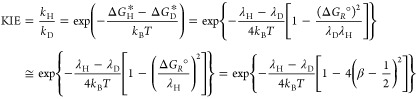6.27

where |ΔG_R°| ≤ λ_H and the zero-point effects are included in the intrinsic barriers. The different masses of H and D lead to different vibrational frequencies for the respective chemical bonds (and thus also to different zero-point energies). Using isotope-dependent reorganization energies in Marcus-style transfer rate expressions will be justified below (see sections 10–12).

The approximation in the second line of eq 6.27 neglects second-order terms in λ_D – λ_H. Substitution of ΔG_R°/λ_H with its expression derived from eq 6.24 leads to the final form of the rate ratio in eq 6.27. As a reaction series is spanned by chemical substitution in A₁ or A₂, the plot of k_H/k_D vs pK_H = (2.303 k_BT)⁻¹ΔG° ≅ (2.303 k_BT)⁻¹ΔG_R° goes through a maximum for β = 1/2 (where Q_t is midway between the reactants and products). The smaller the λ_H value, the sharper (and therefore more discernible experimentally) the peak in the plot of k_H/k_D vs pK_H. Equation 6.27 is not applicable when the second term on the right side of eq 6.25 (neglected in eq 6.24) is appreciable. Moreover, limitations in the applicability of eq 6.27 arise when the reactants and products in eqs 6.26a and 6.26b are not well-characterized by the simple parabolic potentials of the Marcus electron transfer theory. Marcus showed that the effects of this intrinsic barrier asymmetry can be corrected approximately using the mean value of the reorganization energies for the forward and backward reactions.²⁶⁵ The applicability of the extended Marcus theory to the interpretation of experimental data is limited by the fact that nuclear tunneling is not included in the theory. Nuclear/atomic tunneling effects are discussed in the following sections, where PCET theories are analyzed with the unified framework of section 5, which can be of use in interpreting the growing experimental data on PCET reaction mechanisms relevant to biology, medicine, biochemistry, and molecular electronics.

7. Beyond Marcus Theory: Nuclear Tunneling and Structural Constraints on PCET

Marcus theory (as developed for outer-sphere ET and extended to other reactions characterized by strong charge/atom donor–acceptor wave function overlap), and especially the Marcus cross-relation, is used to interpret dissociative ET,^266−269 PT,^{254,270−275} HAT,^{190,253,254,272,276−279} PCET,^{4,116,188−191,196,214,225,229,254,272,280} and hydride transfer reactions.^250,279,281 The success of the Marcus theory applied to such diverse transfer processes lies in its simplicity, the possibility for empirical adjustment of its key parameters,²⁷¹ the generic character of part of the extended theory (e.g., see the last term on the right side of eq 6.25), and the fact that minor deficiencies of the theory may be not detectable.^272,277 The remarkable success (no worse than for outer-sphere ET processes in some cases^272,279,282) of the cross-relation for describing HAT has also been observed in very recent studies and was related to the accuracy of the additivity postulate in eq 6.3 over a wide range of reaction and solvation conditions.^248,279 Yet the physical origins of additivity lie in the weak interactions between the donor and acceptor at relatively long ET distance. Here, the reorganization energy is an additive property of the donor and acceptor. Partial justification of using eq 6.3 to describe heavy-particle transfer and possible reasons for its failure have been addressed by Marcus.²³² However, the broad validity of eq 6.3 presents an open theoretical question. Moreover, for hydride transfer^281,283 and S_N2 reactions^284,285 the validity of eq 6.3 is limited to a narrow set of reactants and reaction mechanisms.

As emphasized by Mayer and co-workers,²⁷² the successful application of the Marcus cross-relation requires additional theoretical-computational modeling of features specific to the reaction system under study, in order to adequately fit the physical parameters that appear in the cross-relation to the experimental data for the reaction. Further modeling by Mayer and co-workers is based on the following main differences between ET and PT or HAT:²⁷⁹ (i) The precursor and successor complexes of an ET reaction²³⁸ can be weakly associated. Each complex’s structure is determined largely by the electrostatic interaction between the reagents (described by the work terms). Instead, HAT requires a more specifically defined geometry of the two association complexes, with close approach of the proton (or atom) donor and acceptor, as a consequence of the larger mass for a tunneling proton or atom. (ii) For PT or HAT reactions, large solvent effects arise not only from the polarization of the solvent (which is generally small for HAT), but also from the ability of the solvent molecules to bond to the donor, thus making it unreactive. This is the predominant solvent effect for HAT reactions, where solvent polarization interacts weakly with the transferring neutral species. Thus, successful modeling of a PT or HAT reaction requires specific modeling of the donor desolvation and precursor complex formation. A quantitative model for the kinetic solvent effect (KSE) was developed by Litwinienko and Ingold,²⁸⁶ using the H-bond empirical parameters of Abraham et al.^287−289 Warren and Mayer complemented the use of the Marcus cross-relation with the KSE model to describe solvent hydrogen-bonding effects on both the thermodynamics and kinetics of HAT reactions.²⁹⁰ Their approach also predicts HAT rate constants in one solvent by using the equilibrium constant and self-exchange rate constants for the reaction in other solvents.^{248,272,279,290}

The success of the combined cross-relation–KSE approach for describing HAT reactions arises from its ability to capture and quantify the major features involved: the reaction free energy, the intrinsic barriers, and the formation of the hydrogen bond in the precursor complex. Factors not accounted for in this approach can lead to significant deviations from the predictions by the cross-relation for a number of HAT reactions (for reactions involving transition-metal complexes, for example).^291,292 One such factor arises from structures of the precursor and successor complexes that are associated with considerable differences between the transition-state structures for self-exchange and cross-reactions. These differences undermine the assumption that underlies the Marcus cross-relation. Other important factors that weaken the validity of the cross-relation in eqs 6.4–6.6 are steric effects, nonadiabatic effects, and nuclear tunneling effects. Nuclear tunneling is not included in the Marcus analysis and is a critical contributor to the failure of the Marcus cross-relation for interpreting HAT reactions that involve transition metals. Isotope effects are not captured by the cross-relation–KSE approach, except for those described by eq 6.27.²⁷² Theoretical treatments of coupled ET–PT reactions, and of HAT as a special case of EPT, that include nuclear tunneling effects will be discussed in the sections below. Understanding the reasons for the success of Marcus theory to describe proton and atom transfer reaction kinetics in many systems is still a fertile area for research.

The role of proton tunneling often defines a large difference between pure ET and PCET reaction mechanisms. This important difference was highlighted in the model for EPT of Georgievskii and Stuchebrukhov.¹⁹⁵ The EPT reaction is described along the diabatic PESs for the proton motion. The passage of the system from one PES to the other (see Figure 28) corresponds, simultaneously, to switching of the localized electronic state and tunneling of the proton between vibrational states localized in the two PESs. These vibrational states are indistinguishable from the eigenstates of the separated V₁ and V₂ potential wells in Figure 28 for proton levels sufficiently deep inside the wells. The proton tunneling distinguishes this EPT mechanism from pure ET assisted by a vibrational mode, where the ET is accompanied by transitions between nuclear vibrational states that do not correspond to different localizations for the nuclear mode. A useful step toward a description of proton tunneling appropriate for use in PCET theories appears in the simple PT model of ref (293), where a Landau–Zener strategy is used to establish the degree of electronic adiabaticity for the PT process. A full extension of the Landau–Zener approach for the interpretation of coupled ET and PT was provided by Georgievskii and Stuchebrukhov.¹⁹⁵

Figure 28.

Effective potential energy profiles for the proton motion in the Georgievskii–Stuchebrukhov model of EPT. The marked regions are as follows: DW = donor well. In this region, the BO approximation is used and the electronically adiabatic potential for proton motion is approximated as harmonic. DB = donor barrier. This represents the classically forbidden region on the left side of the PES crossing point (i.e., x_c in the notation of the reported figure) where the top of the barrier is located. AB = acceptor barrier. AW = acceptor well. Reprinted with permission from ref (195). Copyright 2000 American Institute of Physics.

The study of Georgievskii and Stuchebrukhov defines the probability amplitude for finding the proton at a given position (as in eq B1) and the electron in either diabatic state. This probability amplitude is quantified by dividing the proton coordinate range into four regions (Figure 28) and finding an approximate solution for the probability amplitude in each region. The procedure generates the initial and final localized electron–proton states and their vibronic coupling W_IF through the related tunneling current.^195,294 The resulting form of W_IF is

7.1

In eq 7.1, W_IF^ad is the (double) tunneling matrix element for the electronically adiabatic reaction, where only the lower electronic PES is involved. In this electronically adiabatic limit, the proton tunneling matrix element (that is, W_IF) is evaluated using standard methods.^295,296 In particular, in the WKB approximation,²⁰² the vibronic coupling for the transition between the proton vibrational ground states of the two wells is¹⁹⁵

7.2

Here, ω_D and ω_A are the vibrational frequencies in the wells corresponding to localization of the electron on its donor or acceptor, R_D and R_A are the turning points for classical motion with energy equal to the tunneling energy E (x rather than R denotes the proton coordinate in the reported Figure 28), m_p is the proton mass, and V(R) is the lower adiabatic potential energy. The κ factor in eq 7.1 is¹⁹⁵

7.3

where Γ is the Γ function and p is the proton adiabaticity parameter

7.4

V_IF is the electronic coupling matrix element, ΔF is the difference in slope of the PESs at the crossing point R_t (where the potential energy is V_c), and v_t is the “tunneling velocity” of the proton at this point, defined consistently with Bohm’s interpretation of quantum mechanics²²³ as

7.5

In the electronically adiabatic limit (p ≫ 1), Stirling’s formula applied to eq 7.3 leads to κ = 1, which means that W_IF = W_IF^ad. In the electronically nonadiabatic limit, p ≪ 1, eq 7.3 gives κ = (2πp)^1/2 and substitution into eq 7.1 yields the vibronic coupling in the form expected from the analysis of section 5 (see, in particular, eq 5.41a), namely¹⁹⁵

7.6

S_IF^p is the overlap between the initial and final proton wave functions. The parameter p is like the Landau–Zener parameter used in ET theory, and its interpretation follows along the same lines. In fact, once a proton tunneling “velocity” is defined, p is determined by the speed of the proton “motion” across the region where the electron transition may occur with appreciable probability (the electronic energy matching window). The width of this region is estimated as

7.7

and the proton “tunneling time” is defined as

7.8

The Heisenberg uncertainty principle gives a time lapse for the electronic state change as

7.9

Thus, as in the context of ET,¹⁵⁹p is given by the ratio

7.10

An application of this formalism appears in section 12. The vibronic coupling depends on the mass of the heavy tunneling particle (which may be deuterium or tritium as well) throughout the range of electronically adiabatic-to-nonadiabatic behavior for a given reaction. For the adiabatic limit, in the WKB approximation, the coupling depends exponentially on the square root of the heavy particle mass. The same kind of dependence on the mass arises in the nonadiabatic limit. In this regime, the vibronic coupling is given by eq 7.6, where S_IF^p may be computed as for two displaced harmonic oscillators with frequency ω_p and displacement R̅_DA (i.e., the equilibrium proton donor–acceptor distance):

7.11

where ω_p ≈ 1/(m_p)^1/2. These simple arguments indicate that, whatever the degree of electronic adiabaticity, the W_IF dependence on the mass of the heavy particle is

7.12

where z depends on the electronic adiabaticity of the HAT or PCET reaction. The mass dependence in eq 7.12 leads to a kinetic isotope effect that is absent in eq 6.27 and that may be the major contribution to the effect, especially at low temperatures, where tunneling through the reaction barrier may dominate thermal activation.

Considering the large difference between the proton (or atom) and electron masses, and the exponential decay of S_IF^p with increasing mass, eq 7.11 expresses the importance of achieving appropriate (compressed) proton donor–acceptor distances to favor tunneling, which is a common motif in many enzymes, for example. Useful information on the relationship between structure, structural fluctuations, and functionality was provided in recent studies of Klinman²⁹⁷ that suggest the following model for proton-coupled enzyme catalysis. Increasing the temperature to enter the range where a thermophilic enzyme functions will similarly increase the overall flexibility of the protein, and thus its exploration of conformational space (preorganization). Conformational change is needed to attain catalytically relevant, closely packed active sites. These packed geometries will be characterized by suitable donor–acceptor distances for the relevant charge-transfer reactions and structural rigidity that reduces the local conformational sampling to the most convenient conformations, thus reducing accordingly the reorganization energy. The data in ref (297) support this inverse relationship between protein flexibility and active-site compression.

Connections between charge transfer and interconversion among locally stable conformations of the reactive system have been studied theoretically by Hoffman and Ratner in the context of long-range intramolecular ET.²⁹⁸ They found that the concerted change of conformation and electronic state is always characterized by higher activation energies than the sequential mechanism where either the conformational change or the ET occurs first. Thus, the sequential mechanism is favored and brings about reaction gating. This model does not rely on a specific expression for the ET rate constant. The extension of the model to other charge-transfer reactions allows one to draw connections with the catalytic reaction model in ref (297), because the conformational rearrangements leading to conformations that favor ET can be interpreted as preorganization.

The preference for sequential over concerted mechanisms does not apply more generally to cases where the two processes are both charge transfer reactions. In these cases, the two reactions are reciprocally affected by the electrostatic interaction between the transferring charges. Moreover, the energetics of the nuclear rearrangements accompanying the two processes are both classifiable as reorganization energies (while, in the model of Hoffman and Ratner, one of the two processes may be characterized as a preorganization). An example of preference for the concerted mechanism in an ET–PT reaction is shown in Figure 29. Self-exchange between high-spin iron complexes of 2,2′-biimidazoline, namely, [Fe^II(H₂bim)₃]²⁺ and [Fe^III(H₂bim)₃]³⁺, was studied in ref (229) using dynamic NMR line-broadening techniques. As shown in ref (299), the [Fe^III(Hbim)(H₂bim)₂](ClO₄)₂ complex, where one of the biimidazoline ligands is deprotonated, oxidizes hydrocarbons with weak C–H bonds via a mechanism that is best described as hydrogen atom abstraction. Therefore, this complex can be used to model the function of nonheme iron-containing enzymes that mediate HAT.²²⁹ Biimidazoline ligands are used in ref (229) as models for histidine residues that are often involved in enzymatic PCET reactions.

Figure 29.

Mechanisms for electron–proton transfer in biomimetic iron complexes investigated in ref (229). Reprinted from ref (229). Copyright 2000 American Chemical Society.

Theoretical analysis of the experimental data, with the aim of interpreting the reaction mechanism and differentiating between HAT and coupled (but distinguished) ET and PT events, indicates that both ET/PT (case b in Figure 29) and PT/ET (case c) require overcoming a significantly higher barrier than for the concerted mechanism (depicted in case a). The experimental data do not reveal the timing of ET and PT, but allow one to rule out the existence of the intermediate state shown in the lower panel of Figure 29. HAT is assumed in ref (229) to be the operative concerted mechanism, while theoretical analysis in ref (196) leads to a significant reorganization energy for the concerted reaction, thus suggesting an EPT mechanism.

The example of Figure 29 also highlights the distinction between concerted and sequential PCET mechanisms based on the presence or absence of a stable intermediate. Although the minimum in the sequential model of Figure 29 appears deep enough to allow the detection of an intermediate, its rate of formation is hindered by high flanking free energy barriers.

A great variety of PCET mechanisms arises from the interplay of the relative time scales for transferring electrons and protons and from the couplings among these degrees of freedom.¹⁸² Understanding these diverse time scales and processes requires the identification of the active chemical components of a PCET system and investigation of the relevant structural properties, such as the distances among the electron/proton redox partners and the modulation of these distances by nuclear motion. The kinetic mechanism is simpler when the time scales for ET and PT processes are well separated, and the analysis of this case is addressed in the next section.

8. Proton-Activated Electron Transfer: A Special Case of Separable and Coupled PT and ET

PCET requires interdependence between the ET and PT processes; the charge transfers can take place in a concerted or sequential process.¹⁸⁹ The theoretical description of the coupling between PT and ET is simplified when a sequential mechanism (PT/ET or ET/PT) is experimentally determined. However, the kinetic complexities inherent in biological systems often hinder appreciation of the operative reaction mechanism and thus its theoretical analysis. A special class of PTET reactions is represented by proton-activated electron transfer (PAET). This special class of PT/ET processes was observed, and examined theoretically, in energy conversion processes in the reaction centers of photosynthetic bacteria,^300,301 including the Q-cycle of the cytochrome bc₁ complex, where oxidation/reduction of quinones takes place.^255,302 More generally, biologically relevant long-range ET (which is essential in respiration, photosynthesis, and metabolism) requires protein binding, conformational change, and chemical transformations that include PT to optimize interactions among distant redox partners. Kinetic complexity is introduced by the range of accessible geometries, which complicates the mechanistic interpretation. In PAET, or in the opposite limit of gated ET,^303,304 kinetic complexity is introduced^303,304 into the kinetic scheme

8.1

(where diffusion is followed by the ET reaction between the A and B species) via the more complicated kinetic model

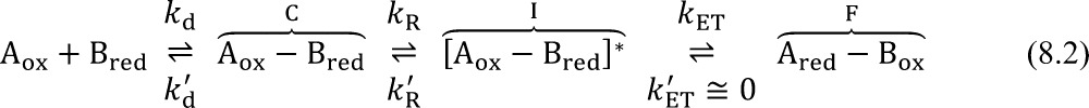8.2

In eq 8.2, a catalytic step yields an efficient ET complex. Of relevance here are circumstances where PT is the catalytic event, or is a crucial part of it (also see the discussion of a similar kinetic model in ref (127), where the focus is on ET reactions, so the reorganization from the inefficient precursor complex C to the efficient ET complex I does not involve PT). Although the PT and ET events are coupled, they are kinetically separable when each PT step is much faster than ET. If the proton configuration required for ET is unfavorable, as reflected in an equilibrium constant K_R = k_R/k_R′ ≪ 1, the “electron transfer is convoluted with a weak occupancy of the proton configuration needed for electron transfer”.²⁵⁵ In this case, the kinetic equations under steady-state conditions (and with a negligible rate for reverse ET) lead to^305,306k_obsd = K_Rk_ET. The combination of this result with the Brønsted relationship²⁴¹ and a Marcus-type expression for the ET rate^7,307 yields an expression for k_obsd that allows comparison with experimental data, identification of the free energy contributions from the PT and ET processes, and the useful interpretation of enzymatic mechanisms.^255,302

We now sketch an alternative, simple derivation of such an expression. For the reaction mechanism of eq 8.2, under steady-state conditions and without considering the diffusion process (characterized by the rate constants k_d and k′_d in eqs 8.1 and 8.2), C and F represent (using a language familiar from molecular electronics¹⁴⁹) constant source and drain for the observed ET reaction starting from the inefficient precursor complex C. The stationary flux J of electron charge per redox couple can be expressed in terms of both k_obsd and the rate k_ET for the true ET step as

8.3

where the P_C and P_I are the occupation probabilities of states C and I, respectivley, of the redox system. By applying detailed balance and rewriting in terms of the concentrations [C] and [I], one finds

8.4

By inserting eq 8.4 and the Marcus ET rate (without work terms) into eq 8.3

8.5

where υ is derived from the Marcus ET rate. Indeed, refs (255) and (302) use the generalization of the Marcus ET rate expression provided by Hopfield,³⁰⁸ as parametrized by Dutton and Moser,^309−311 so that k_obsd is given, in units of inverse seconds, as

8.6a

with

8.6b

where r is the edge-to-edge distance between the protein ET donor and acceptor, and β_ET is an average decay factor of the squared electronic coupling. ı is numerically equal to 3.1, and hence, it differs from 1/(4k_BT) over the whole range from 0 °C to room temperature. The difference between eqs 8.5 and 8.6 is significant in two respects: eq 8.6, compared to eq 8.5, reflect a partial correction for nuclear tunneling to the Marcus ET rate and makes explicit the dependence of the ET rate constant on r.

When there are thermally populated nuclear frequencies ω_n with ℏω_n ≥ k_BT that are relevant to ET, a quantum (or at least semiclassical) treatment^152,308,312 of the nuclear modes is important, although in some regimes the quantum expressions of the ET rate preserve a near-Gaussian dependence on ΔG°, similar to the Marcus expression. Indeed, the same Gaussian free energy dependence as in Marcus theory was obtained by Hopfield,³⁰⁸ but k_BT was replaced by (1/2)λℏωcoth(ℏω/2k_BT), where ω is the effective frequency of the nuclear oscillator.³⁰⁸ At high temperature, it is coth(ℏω/2k_BT) ≅ 2k_BT/ℏω and the Marcus ET rate expression is recovered. At low temperature (where the donor–acceptor energy fluctuations may become correlated, so the use of the Hopfield formulation of the ET rate may be limited, although it correctly predicts the transition to a temperature-independent tunneling regime^308,312,313), coth(ℏω/2k_BT) ≅ 1 so that the expression for the ET rate vs ΔG° is a Gaussian function with variance essentially independent of T and approximately given by λℏω. In this limit, the tunneling of nuclei is important and can give rise to significant isotope effects. In general, the contribution of quantum nuclear modes needs to be accounted for in the evaluation of the reorganization energy, which can require an improved treatment of the coupled PT and ET, especially where the two events cannot be separated and the main role of PT cannot be described by a probability distribution, as in the derivation of eq 8.6. This point is explored in the sections below.

The consideration of ET pathways and their interferences^314,315 allows the interpretation of experiments where the structural features crucial to ET or PCET matrix elements are of interest. In this regard, an emblematic case is offered by recent experiments involving mutations and kinetic studies on the enzyme tyramine β-monooxygenase,³¹⁶ where the aromatic ring of the amino acid Tyr216 may mediate a long-range interdomain ET process crucial to the enzymatic mechanism,³¹⁷ and the Tyr-to-Ala mutation causes a drastic decrease in the observed ET rate.³¹⁶ In agreement with this observation, a previous theoretical investigation of the corresponding ET step in the related enzyme peptidylglycine α-hydroxylating monooxygenase³¹⁸ identified an efficient ET pathway through a network of hydrogen and covalent bonds, and residues at the enzyme active site, that is assisted by the formation of structured water, with an expected increase in electron tunneling efficiency compared to that of bulk water.³¹⁹ In the study of ref (318) it was assumed that the reorganization energy was not affected by the mutations, but further analysis of a possible connection between the water structuring and the reorganization energy would be useful. In the theoretical study, the hydrogen atoms were added by assigning the protonation states of all ionizable groups. Future extension of this analysis to include the possibility for PCET is important in light of recent studies that propose a PCET mechanism for the process³²⁰ (the mechanism proposed in ref (320) is based on a long-distance ET step coupled to many short-distance PT steps, described as hydrogen atom transfer along a chain of structured waters).

The discussion above highlights the fact that fruitful exploration of ET and PCET mechanisms is possible using modern theoretical methods.^321−323 Such studies impact biology,^{316,318,323−325} electrochemistry,³²⁶ and molecular electronics.³²⁷ In particular, opportunities exist to use the theory of PCET reactions to identify the proton donors and acceptors, as well as the timing and coupling of the PT and ET events.^328−330 Moreover, the de novo design of bioinspired artificial catalytic systems requires that structural and functional information provided by the natural enzymes is augmented by “a practical sense of structural and energetic engineering tolerances of the mechanism”,³³¹ exemplified by the recent design of peptide-incorporated naphthoquinone amino acids that perform reversible PCET.³³²

It is worth noting that PCET includes PAET as a special case. More specifically, PAET is a type of PT/ET reaction (see section 5), In fact, the occurrence of the ET is enabled by the PT step; hence, the two events are coupled, even though the separation in time scales does not lead to concerted electron and proton charge redistributions. In general, kinetic and thermodynamic investigations will establish the mechanisms at play in the given system, as discussed further below.

9. Dogonadze–Kuznetsov–Levich (DKL) Model of PT/HAT and Connections with ET and PCET Theories

Dogonadze, Kuznetsov, and Levich have also developed a theoretical description of PT reactions as an extension of their previous theories of outer-sphere ET.^178−180 Their theoretical model was first applied to PT at electrodes and then to homogeneous PT reactions such as

9.1

A significant feature of this model, adopted in subsequent PCET theories, is a generalized use of the BO separation scheme, in which adiabatic (or standard BO) and double-adiabatic approximations are distinguished. This treatment begins by considering the frequencies of the system: ω₀ describes the motion of the medium dipoles, ω_p describes the frequency of the bound reactive proton in the initial and final states, and ω_e is the frequency of electron motion in the reacting ions of eq 9.1. On the basis of the relative order of magnitudes of these frequencies, that is, ω₀ ≈ 10¹¹ s^–1 ≪ ω_p ≈ 10¹⁴ s^–1 ≪ ω_e ≈ 10¹⁵ s^–1, two possible adiabatic separation schemes are considered in the DKL model: (i) The electron subsystem is separated from the slow subsystem composed of the (reactive) proton and solvent. This is the standard adiabatic approximation of the BO scheme. (ii) Aside from the standard adiabatic approximation, the transferring proton also responds instantaneously to the solvent, and a second adiabatic approximation is applied for the proton dynamics.

In both approximations, the fluctuations of the solvent polarization are required to surmount the activation barrier. The interaction of the proton with the anion (see eq 9.2) is the other factor that determines the transition probability. This interaction appears as a perturbation in the Hamiltonian of the system, which is written in the two equivalent forms

9.2

by using the unperturbed (channel) Hamiltonians and for the system in the initial and final states, respectively. q_A and q_B are the electron coordinates for ions A^– and B^–, respectively, R is the proton coordinate, Q is a set of solvent normal coordinates, and the perturbation terms V_pB and V_pA are the energies of the proton–anion interactions in the two proton states. includes the Hamiltonian of the solvent subsystem, as well as the energies of the AH molecule and the B^– ion in the solvent. is defined similarly for the products. In the reaction of eq 9.1, V_pB determines the proton jump once the system is near the transition coordinate. In fact, Fermi’s golden rule gives a transition probability density per unit time

9.3

where Ψ_I⁰ and Ψ_F are unperturbed wave functions for the initial and final states, which belong to the same energy eigenvalue, and ρ_F is the final density of states, equal to 1/(ℏω₀) in the model.

The rate of PT is obtained by statistical averaging over initial (reactant) states of the system and summing over final (product) states. Equation 9.3 indicates that the differences between models i and ii arise from the strategies used to write the wave functions, which reflect the two different levels of approximation to the physical description of the system. Using the standard adiabatic approximation, Ψ_I⁰ and Ψ_F in the DKL model are written as

9.4a

9.4b

where ϕ_A(q_A,R,Q)ϕ_B(q_B,Q) and ϕ_A(q_A,Q)ϕ_B(q_B,R,Q) are the electronic wave functions for the reactants and products, respectively, and χ_A (χ_B) is the wave function for the slow proton–solvent subsystem in the initial and final states, respectively. The notation for the vibrational functions emphasizes^179,180 the dependence on the different proton localizations before and after the transfer reaction. The initial and final PESs in the DKL model are elliptic paraboloids in the two-dimensional space of the proton coordinate and a collective solvent coordinate (see Figure 18a). The reaction path on the PESs is interpreted in the DKL assumption of negligible solvent frequency dispersion.

Two assumptions simplify the computation of the PT rate in the DKL model. The first is the Condon approximation,^117,159 neglecting the dependence of the electronic couplings and overlap integrals on the nuclear coordinates.³³³ The coupling between initial and final electronic states induced by V_pB is computed at the R and Q values of maximum overlap integral for the slow subsystem (R_t and Q_t). The second simplifying approximation is that both the proton and solvent are described as harmonic oscillators, thus allowing one to write the (normal mode) factored nuclear wave functions as

9.5

The PT matrix element is given by

9.6a

with

9.6b

9.6c

9.6d

The rate of PT is obtained by statistical averaging over initial (reactant) states of the system and summing over final (product) states.

The factored form of the proton coupling in eqs 9.6a–9.6d leads to significant simplification in deriving the rate from eq 9.3 because the summations over the proton and solvent vibrational states can be carried out separately. At room temperature, ℏω_p > k_BT, so the quantum nature of the transferring proton cannot be neglected despite approximation i.³³⁴ The fact that ℏω₀ ≪ k_BT (high-temperature limit with respect to the solvent), together with the vibrational mode separation of eqs 9.6a–9.6d, validates the classical limit for the solvent degrees of freedom and leads to the rate^180,335

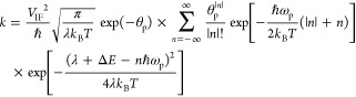9.7

In eq 9.7, θ_p is a (dimensionless) measure of the coupling between the proton and the other degrees of freedom that is responsible for the equilibrium distance R̅_AB between the proton donor and acceptor:

9.8

Here, m_p is the proton mass. λ is the solvent reorganization energy for the PT process:

9.9

where Q̅_kA and Q̅_kB are the equilibrium generalized coordinates of the solvent for the initial and final states. Finally, ΔE is the energy difference between the minima of two PESs as in Figure 18a, with the value

9.10

Here, ε_B(R̅_B,Q̅_B) and ε_A(Q̅_B) are the energies of the solvated molecule BH and ion A^–, respectively, at the final equilibrium geometry of the proton and solvent, and ε_A(R̅_A,Q̅_A) and ε_B(Q̅_A) are the respective quantities for AH and B^–. The energy quantities subtracted in eq 9.10 are introduced in refs (179) and (180) as potential energies, which appear in the Schrödinger equations of the DKL treatment.¹⁷⁹ They may be interpreted as effective potential energies that include entropic contributions, and hence as free energies. This interpretation has been used consistently with the Schrödinger equation formalism in elegant and more general approaches of Newton and co-workers (in the context of ET)³³⁶ and of Hammes-Schiffer and co-workers (in the context of PCET; see section 12).^214,337 In these approaches, the free energy surfaces that are involved in ET and PCET are obtained as expectation values of an effective Hamiltonian (see eq 12.11).

Returning to the analysis of the DKL treatment, another approach to obtain the charge transfer rate in the above theoretical framework uses the double-adiabatic approximation, where the wave functions in eqs 9.4a and 9.4b are replaced by

9.11a

9.11b

The electronic components are parametric in both nuclear coordinates, and the proton wave function also depends parametrically on Q. To obtain the wave functions in eqs 9.11a and 9.11b, the standard BO separation is used to calculate the electronic wave functions, so R and Q are fixed in this computation. Then Q is fixed to compute the proton wave function in a second adiabatic approximation, where the potential energy for the proton motion is provided by the electronic energy eigenvalues. Finally, the Q wave functions for each electron–proton state are computed. The electron–proton energy eigenvalues as functions of Q (or electron–proton terms) are one-dimensional PESs for the Q motion (Figure 30). A procedure similar to that outlined above, but without the harmonic approximation for the proton states and the Condon approximation, gives the rate¹⁸⁰

9.12a

where P_μ is the Boltzmann probability of the μth proton state in the reactant electronic state (with associated vibrational energy level ε_Iμ^p):

9.12b

Z_I^p is the partition function, ε_Fν is the proton vibrational energy in the product electronic state, W_μν is the vibronic coupling between initial and final electron–proton states, and ΔE is the fraction of the energy difference between reactant and product states that does not depend on the vibrational states. Analytical expressions for W_μν and ΔE are provided in the theory.^179,180 The same result as in eq 9.7 is recovered if the initial and final proton states are again described as harmonic oscillators with the same frequency and the Condon approximation is applied (see also section 5.3).

Figure 30.

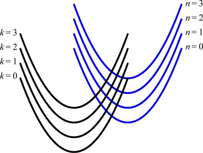
Diabatic electron–proton PFESs as functions of the classical nuclear coordinate Q. This one-dimensional landscape is obtained from a two-dimensional landscape as in Figure 18a by using the second BO approximation to obtain the proton vibrational states corresponding to the reactant and product electronic states. Since PT reactions are considered, the electronic states do not correspond to distinct localizations of excess electron charge.

In the DKL treatment¹⁸⁰ it is noted that the sum in eq 9.7, evaluated at the different values of ΔE, has a dominant contribution that is usually provided by a value n̅ of n such that³³⁸

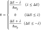9.13

Indeed, for a given ΔE value, eq 9.13 yields a real number n̅ that corresponds to the maximum of the curve interpolating the values of the terms in sum, so that it can be used to produce the following approximation of the PT rate:

9.14a

where the Poisson distribution coefficient is

9.14b

and the activation energy is

9.14c

The PT rate constant in the DKL model, especially in the form of eq 9.14 resembles the Marcus ET rate constant. However, for the PT reaction studied in the DKL model, the activation energy is affected by changes in the proton vibrational state, and the transmission coefficient depends on both the electronic coupling and the overlap between the initial and final proton states. As predicted by the Marcus extension of the outer-sphere ET theory to proton and atom transfer reactions, the difference between the forms of the ET and PT rates is minimal for |ΔE| ≤ λ, and substitution of eq 9.13 into eq 9.14 gives the activation energy

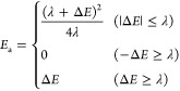9.15

Apart from the dependence of the energy quantities on the type of charge transfer reaction, the DKL theoretical framework may be applied to other charge-transfer reactions. To investigate this point, we consider, for simplicity, the case |ΔE| ≤ λ. Since ℏω_p is larger than the thermal energy k_BT, the terms in eq 9.7 with n > 0 are negligible compared to those with n < 0. This is an expression of the fact that a higher activation energy is necessary for the occurrence of both PT and excitation of the proton to a higher vibrational level of the accepting potential well. As such, eq 9.7 can be rewritten, for many applications, in the approximate form

9.16

where the summation was extended to the n ≤ 0 terms in eq 9.7 (and the sign of the summation index was changed).

The electronic charge distributions corresponding to ϕ_A and ϕ_B are not specified in eqs 9.4a and 9.4b, except that their different dependences on R are included. If we assume that ϕ_A and ϕ_B are characterized by distinct localizations of an excess electron charge (namely, they are the diabatic states of an ET reaction), eq 9.16 also describes concerted electron–proton transfer and, more specifically, vibronically nonadiabatic PCET, since perturbation theory is used in eq 9.3. Using eq 9.16 to describe PCET, the reorganization energy is also determined by the ET. Equation 9.16 assumes ℏω_p ≫ k_BT, so the proton is initially in its ground vibrational state. In our extended interpretation, eq 9.16 also accounts for the vibrational excitations that may accompany³³⁹ an ET reaction. If the different dependences on R of the reactant and product wave functions in eqs 9.4a and 9.4b are interpreted as different vibrational states, but do not correspond to PT (thus, eq 9.1 is no longer the equation describing the reaction), the above theoretical framework is, indeed, unchanged. In this case, eq 9.16 describes ET and is identical to a well-known ET rate expression^339−342 that appears as a special case for ω₀ ≪ k_BT/ℏ ≪ ω_p in the theory of Jortner and co-workers.³⁴³ The frequencies of proton vibration in the reactant and product states are assumed to be equal in eq 9.16, although the treatment can be extended to the case in which such frequencies are different.

In both the PT and PCET interpretations of the above theoretical model, note that θ_pⁿexp(−θ_p)/n! is the overlap between the initial and final proton wave functions, which are represented by two displaced harmonic oscillators, one in the ground vibrational state and the other in the state with vibrational quantum number n.³⁴⁴ Thus, eq 9.16 can be recast in the form

9.17a

with vibronic coupling

9.17b

This expression is similar to that obtained in the general context of PCET by Cukier (for example, see eq 2.9 in ref (116)) and by Soudackov and Hammes-Schiffer, for cases where the proton is initially in its vibrational ground state, since ℏω_p ≫ k_BT, and the reorganization energies associated with the different transitions in eq 9.17a are dominated by a similar solvent contribution.^191,337 In this limit for λ and the classical limit for the solvent modes, the effect of proton donor–acceptor distance (X ≡ R_AB) fluctuations on S_0n^p can be included in the rate expression of eq 9.16 or eq 9.17. X is one of the two nuclear coordinates considered in the PT and HAT theory of refs (165) and (192), where the other nuclear coordinate, S, is the solvent coordinate responsible for the outer-sphere contribution to λ. The formalism of refs (165) and (192) was extended to the theoretical investigation of PCET reactions (thus including HAT as a special case) in recent studies of Hammes-Schiffer and co-workers, where X was added to a set of two collective nuclear coordinates^337,345 (Q and S). Since S_0n (similarly to the coupling in pure nonadiabatic PT) decreases exponentially with X

9.18

the average of |S_0n^p(X)|² using the probability density of the X classical oscillator

9.19

(M and ω are the mass and frequency of the oscillator) is obtained from the integral³⁴⁶

9.20

as

9.21

Using this average overlap rather than eq 9.18 in eq 9.17a, one finds

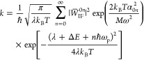9.22

which can be obtained, for the conditions in the above model (BO adiabatic approximation, initial and final proton vibrations of equal frequency, and temperatures such that ω₀ ≪ k_BT/ℏ ≪ ω_p), within the theoretical frameworks of Borgis and Hynes^165,192,193 and of Hammes-Schiffer and co-workers.³³⁷ The possibility of populating different initial vibronic states was also included in these treatments,^228,337,345 using a Boltzmann distribution of the populations. Thermal averaging was also performed by Kuznetsov and Ulstrup,¹⁸¹ with the main focus on PT, concerted electron–proton transfer, and applications to HAT in enzymatic reactions studied by Klinman and co-workers.^347−349 The rate formulated by Kuznetsov and Ulstrup in refs (181) and (350) (see also ref (351)) is

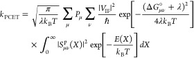9.23a

(note that the Condon approximation is not assumed in ref (350)) with³⁵²

9.23b

where ΔG° corresponds to (and generalizes) the energy difference ΔE of the DKL model. E(X) is the energy that determines the probability density of the distance between the proton donor and acceptor. E(X) may be the energy of the classical X mode leading to eq 9.22 or a different expression depending on the system coordinates related to X (Figure 26). By appropriate expression of E(X), the PCET rate in eq 9.23 can include the effects of solvent modes, as in the studies of Hammes-Schiffer’s group,^184,337,345 and can be applied to gated biological PT reactions.^{351,353−355} Reference (353) investigates, e.g., the case of a proton relay in serine proteases, where a conformationally mobile histidine allows the system to achieve productive PT donor–acceptor distances. The convolution of the charge transfer rate with the probability density for the charge donor–acceptor distance is also generically formulated in the DKL model (see ref (180) and references therein).

10. Borgis–Hynes (BH) Theory for PT and HAT

10.1. Dynamical Regimes of the BH Theory

More than 20 years ago, Borgis and Hynes developed^{165,192,193,228,356} a dynamical theory for the rate of PT and HAT reactions in a partially adiabatic regime that is characterized by an electronic coupling that is large compared to k_BT (electronically adiabatic regime of the reaction) and a vibrational coupling small compared to k_BT (vibronically nonadiabatic regime), as may be found with malonaldehyde and carboxylic acid dimers in polar condensed media. In this regime, the reaction involves nuclear tunneling through an electronically adiabatic potential barrier separating the reactant and product potential wells (see section 5).

Along the solvent coordinate, the vibrationally nonadiabatic PT can be described analogously to (pure) nonadiabatic ET, with a corresponding definition of the effective vibrational coupling as half the splitting between the vibrationally adiabatic ground state and first-excited state energies (or, if one generalizes, the two involved vibrational states), calculated for the lowest electronic adiabatic state. The simultaneous occurrence of ET and PT in HAT, and the equivalence of vibrational and vibronic nonadiabaticity determined by the adiabatic behavior of the electron,¹⁸² allowed the authors to describe the transition without specifying whether the species involved is a proton or a hydrogen atom. Moreover, since the process is electronically adiabatic, in the case of proton transfer, the electronic coordinate can be separated using the BO adiabatic approximation and channel Hamiltonians for reactants and products (with respect to the proton state) can be defined in terms of the nuclear coordinates.^165,193,228 The proton dynamics is fast compared to the relevant intramolecular vibrations and solvent motions far from the avoided crossing of the proton PESs, so the BO adiabatic approximation is valid, and the analogue of eq 5.63 holds for the proton vibrational wave functions in terms of the reactive nuclear coordinates. For HAT, the reactant and product Hamiltonians need to be constructed considering the electronic coordinate or an overall description of the hydrogen atom.

In the BH theory, the coupling between the reactant and product states for PT or HAT is defined from the minimum splitting of the proton or hydrogen atom PESs, and only the exponential decay of the coupling with the donor–acceptor distance is explicitly modeled.¹⁹² The resulting formalism can be applied to electronically adiabatic EPT. In this regard, a recent study¹⁸⁶ refers to the BH reaction rate constant originally obtained for HAT as being an appropriate expression to describe concerted PCET in the partially adiabatic regime (as was defined above). However, EPT can be electronically nonadiabatic in many cases, where, in fact, the electronically adiabatic or nonadiabatic character of the reaction can be used to distinguish between HAT and EPT.^197,215 Even in these cases, the formalism of BH theory holds for a rate expression where the vibrational coupling is replaced by a vibronic coupling between electron–proton states that need to be computed consistently with the nonadiabatic electronic behavior. However, the BH treatment focused on PT and HAT reactions. The validity of a significant part of their formalism in the general PCET context was appreciated later, thanks to the contributions of Hammes-Schiffer and co-workers, which included theoretical development for the appropriate computation of free energies and couplings involved in the PCET reaction rates (see section 12).^{225,337,345,357}

10.2. Splitting and Coupling Fluctuations

In the electronically adiabatic, vibrationally (or vibronically¹⁸²) nonadiabatic case, the transition rate constant is proportional to the square of the vibrational coupling, which depends parametrically on (and thus is modulated by) the fluctuations of the proton donor–acceptor distance X (intramolecular vibration) and of a relevant collective solvent coordinate S. Borgis and Hynes note that¹⁹² their theory makes the most contact with the DKL theory^179,180,358 and with the studies of Ulstrup and co-workers.³⁵⁰ The BH theory, however, differs from these other treatments in its dynamical approach, the treatment of the quantum and dynamical character of the X coordinate, and the simultaneous consideration of the X and S coordinates.

As in the BH analysis, the transferring species, either a proton or hydrogen atom, is denoted here by H. The relevant nuclear coordinates are depicted in Figure 31 and the corresponding free energy landscapes in Figure 32. The harmonic approximation is assumed for the X and S degrees of freedom. The X and S coordinates are characterized by masses M and M_S and by frequencies ω and ω_S, respectively. The reaction free energies or asymmetries along the X and S coordinates are denoted by ΔE_X and ΔE_S, respectively, and the coordinate shifts between the corresponding free energy minima are ΔX and ΔS, which correspond to reorganization free energies λ_X = (1/2)Mω²ΔX² and λ_S = (1/2)M_Sω_S²ΔS².

Figure 31.

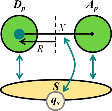
Schematic representation of the system and interactions in the Borgis and Hynes model for HAT and PT. D_p and A_p are the proton (or H atom) donor and acceptor, respectively. R is the coordinate of the H species (cyan circle), and X is the H donor–acceptor distance. S is the solvent coordinate, and q_s denotes the coordinate set of the “infinitely” fast solvent electrons. In the continuum model, the solvent electronic polarization is assumed to be in equilibrium with the charge distribution of the reaction system at all times. The interactions between the components of the solute and the solvent are depicted as double-headed arrows. X vibrations are affected by the stochastic interactions with the solvent, which include short-range (collisional) and electrostatic components. In turn, the D_p–A_p coupling is affected (indirect mechanism). D_p, A_p, and H directly interact with the solvent (direct mechanism).

Figure 32.

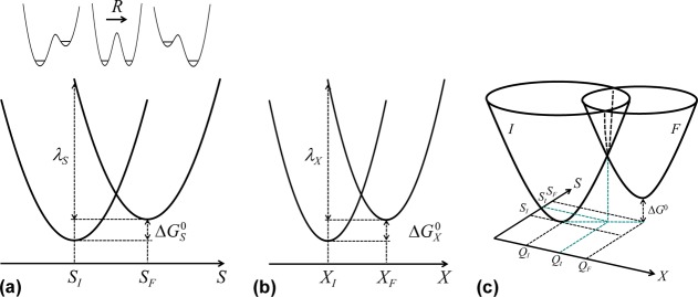
Free energy landscapes for the Borgis–Hynes theory of PT and HAT. (a) Free energy profile for the transferring H species along the solvent coordinate S. The pertinent free energy of reaction or asymmetry ΔG_S° and reorganization energy λ_S are shown. The H double wells at different S values are also depicted. In the model, the activation barrier along the H coordinate (R) is significantly higher than the S-dependent reaction free energy (the asymmetry is magnified in the PESs for the R coordinate of panel a). (b) Free energy profile along the intramolecular coordinate X defining the H donor–acceptor distance. The X dependence of the potential double wells for the H dynamics may be represented as the S dependence in panel a. (c) Full free energy landscape as a function of S and X (cf. Figure 1 in ref (192)).

The BH analysis is first restricted to cases in which only the reactant and product ground H vibrational states are involved in the reaction. In the nonadiabatic limit (the analogue of eq 5.63 with reference to the H coordinate), the splitting between the H levels in reactants and products, as a function of the coordinate changes δX and δS about the equilibrium positions for the reactant state, is given by

10.1a

(mass-weighted coordinates are not used here) where

10.1b

is the total free energy of reaction depicted in Figure 32c. The other terms in eq 10.1a are obtained using Δ₂₁ = −Δ₁₂ in Figure 24 rewritten in terms of X and S. The evaluation of Δ₁₂ at the reactant X and S coordinates yields λ_X and λ_S, while differentiation of Δ₁₂ and expression of ΔX and ΔS in terms of λ_X and λ_S lead to the last two terms in eq 10.1a.

Borgis and Hynes note that two different types of X fluctuations can affect the H level coupling and, as a consequence, the transition rate: (i) coupling fluctuations that strongly modulate the width and height of the transfer barrier and hence the tunneling probability per unit time (for atom tunneling in the solid state, Trakhtenberg and co-workers showed that these fluctuations are thermal intermolecular vibrations that can substantially increase the transition probability by reducing the tunneling length, with particular relevance to the low-temperature regime³⁵⁹); (ii) splitting fluctuations that, as the fluctuations of the S coordinate, modulate the symmetry of the double-well potential on which H moves. A single X coordinate is considered by the authors to simplify their model.^192,193 In Figure 33, we show how a single intramolecular vibrational mode X can give rise to both kinds of fluctuations. In Figure 33, where S is fixed, the equilibrium nuclear conformation after the H transfer corresponds to a larger distance between the H donor and acceptor (as in Figure 32b if X is similarly defined). Thus, beginning at the equilibrium value of X for the initial H location (X = X_I), a fluctuation that increases the H donor–acceptor distance by δX brings the system closer to the product-state nuclear conformation, where the equilibrium X value is X_F = X_I + ΔX. Moreover, the energy separation between the H localized states approaches zero as X reaches the PT transition state value for the given S value (see the blue PES for H motion in the lower panel of Figure 33). The increase in X also causes the the tunneling barrier to grow, thus reducing the proton coupling and slowing the nonadiabatic rate (cf. black and blue PESs in Figure 33). The PES for X = X_F (not shown in the figure) is characterized by an even larger tunneling barrier and lower minimum for R = R_F. A negative δX brings the system farther from the transition coordinate, in the reactant basin (to the left starting from X_I in Figure 32b), with an increase in the energy of the reactants but an even larger increase in the energy of the products. Thus, the decrease in X lowers the tunnel barrier from the side of the product and increases the reaction free energy in favor of the reactants.

Figure 33.

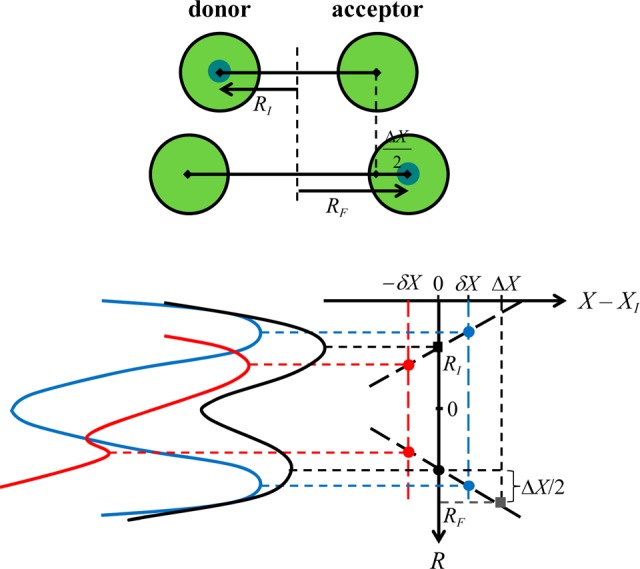
Schematic representation of the dual effect of the proton/hydrogen atom donor–acceptor distance (X) fluctuations on the H coupling and thus on the transition rate. The solvent coordinate S is fixed. The proton coordinate R is measured from the midpoint of the donor and acceptor (namely, from the vertical dashed line in the upper panel, which corresponds to the zero of the R axis in the lower panel and to the top of the H transition barrier for H self-exchange). The initial and final H equilibrium positions at a given X change linearly with X, neglecting the initial and final hydrogen bond length changes with X. Before (after) the PT reaction, the H wave function is localized around an equilibrium position R_I (R_F) that corresponds to the equilibrium value X_I (X_F = X_I + ΔX) of the H donor–acceptor distance. The equilibrium positions of the system in the {X,R} plane before and after the H transfer are marked as black and gray squares. A fluctuation δX > 0 leads to the transition state for PT at the given S (splitting fluctuation yielding the H symmetric PES in blue). The same δX increases the tunneling barrier compared to the PES for H at X = X_I (see PES in black), thus acting as a coupling fluctuation. δX < 0 (smaller distance between the proton donor and acceptor) decreases the tunneling barrier on the proton-state side, which increases in energy compared to the reactant state, therefore inhibiting the transition to the final proton state while ⟨X⟩ = X_I (red PES). In this figure, the X splitting effect is magnified (cf. Figure 34).

The splitting effect of the X displacement was magnified in Figure 33 for visibility. The main effect of X fluctuations is, indeed, the modulation of the H tunneling barrier (see Figure 34), which causes an exponential dependence of the H coupling on the X coordinate value. The fluctuations explore only relatively large X values in the studied nonadiabatic regime. Assuming parabolic diabatic PESs for the R coordinate, and using an approximation such as in eq 5.63 for the ground-state adiabatic PES, the tunneling barrier height has a quadratic dependence on the separation X between the PES minima, while the effects of the X splitting fluctuations are neglected in Figure 34. In the BH model, the asymmetry in the potential double well for the H motion induced by the solvent fluctuations is also weak compared to the potential barrier height for the H transfer reaction.¹⁶⁵ Therefore, the H coupling is approximately independent of the S value. This Condon approximation with respect to the S coordinate reflects the high H tunneling barrier that is assumed in the (vibrationally) nonadiabatic limit considered. The ΔG_X° and ΔG_S° asymmetries can, however, play significant roles in the dynamics of the X and S coordinates, as shown in Figures 32a,b (and in the landscape of Figure 32c), where the reaction free energy is a significant fraction of the reorganization energy. The different significance of the PES asymmetry in the PESs for R and for X and S is understood from the large difference in the typical vibrational frequencies of the respective motions and from eq 5.53, which relates these frequencies to PES curvatures.

Figure 34.

Double-well potential for the H species, at the equilibrium value of X (δX = 0) and after a contraction of the H donor–acceptor distance (δX < 0). The tunneling barrier is reduced by the X fluctuation. The effect on the lowest vibrational levels in the two wells is also shown qualitatively.

The parabolic (harmonic) approximation for the H diabatic PESs does not accurately describe the top of the tunneling barrier. However, the main conclusions drawn above on the X coupling and splitting fluctuations do not depend on the precise shape of the barrier top. For example, near the top of the H tunnel barrier, one may assume a potential energy of the Eckart form³⁶⁰ with parameters dependent on X (see Figure 35):

10.2

Figure 35.

Representation of the Eckart-type potential V(R;X) in eq 10.2 as a function of the proton coordinate R for fixed proton donor–acceptor distance X and the B/A values indicated on the curves.

The potential for the H dynamics differs significantly from this form near the two minima, where the Eckart potential is appropriate for gas-phase proton or atom transfer reactions.²³² Indeed, the Eckart potential was used to model the potential barrier for proton transfer reactions (e.g., see ref (361) and references therein), although the form described here includes a parametric dependence on the X coordinate. In the potential of eq 10.2, X/2 measures the Eckart barrier width. A comparison with a harmonic double well shows that A is a measure of the reaction (free) energy and B may be related to the reorganization energy. The Eckart potential energy has a maximum only if B > A, with a value of (A + B)²/(4B). Thus, the potential barrier height increases with B and becomes nearly independent of A (A is determined by the X splitting fluctuations) for sufficiently large B/A. The modulation of the barrier height by X fluctuations may also be described via this potential model. To this end, appropriate choices of A(X) and B(X) can increase the flexibility of the model in eq 10.2.

As discussed above, the coupling fluctuations of X influence W_IF exponentially.¹⁹³ This is seen by estimating the electron–proton potential energy surfaces^225,362 or using a WKB analysis.^193,202,363 The WKB approximation at the transition-state coordinates X_t and S_t gives^364,365

10.3

where ω_H is the vibrational frequency in each potential well (or, more generally, the geometric average of the frequencies in two wells with different curvatures^193,366,367), m_H is the mass of the tunneling particle, E is the energy of the two H levels, V is the barrier potential, and −a and a are the classical turning points in the two wells (corresponding to the energy E). A small fluctuation δX of the donor from its equilibrium position, where W_IF = W̅_IF, can be described using an expansion of the exponent to first order in δX, giving

10.4

α_IF is in the range of 25–35 Å^–1, to be compared with an order of magnitude of 1 Å for ET, and the approximation holds for moderately to weakly hydrogen-bonded H transfer systems (e.g., for X larger than ∼2.7 Å in OH···O systems).^192,368 For example, as shown by Table 1, proton donor–acceptor distances in this regime may be found in PSII (with a distance of about 2.7 Å between the oxygen on the phenol of TyrD and the nitrogen on the imidazole of H189), in the BLUF domain (see Tyr8 entry in Table 1), and in RNR and photolyase from E. coli (see entries for Trp48 and Trp 306 in Table 1). The much larger value of the vibronic coupling distance decay factor compared to the decay factor for an ET matrix element explains the failure of the Condon approximation for the H coupling in the presence of X fluctuations. However, as a consequence of the BO separation of R and the nuclear X and S coordinates invoked in the BH model, W_IF depends parametrically on X in the expression of the H transfer rate. Furthermore, the X vibration can have classical or quantum mechanical behavior even at room temperature, while S is treated classically.

The large value of α_IF amounts to a large change in the coupling for very small changes in X. Thus, while the splitting effect of the X fluctuations may have a secondary or negligible role in overcoming the activation barrier, their effect on the coupling strongly influences the reaction dynamics near the top of the barrier. In contrast, the fluctuations of the S coordinate have little (neglected in the BH model) influence on the vibronic coupling and a large effect on the activation barrier.

10.3. Reaction Rate Constant

Using the time-correlation function formalism^369,370 and the definition of a negative time-ordered exponential,^371,372 Borgis and Hynes wrote the H transfer rate as

10.5a

with the time correlation function

10.5b

When X is treated quantum mechanically, W_IF(t) and ΔH(τ) are Heisenberg operators for the H coupling and the diabatic energy gap, respectively. The brackets indicate a thermodynamic average taken over the reactant states. The negative time-ordered exponential exp₍₋₎ is defined so that the nth term of its power series expansion is³⁷²

10.6

with τ_n > τ_n–1 > ... > τ₁ throughout each integration interval. We note that eq 10.5 express the rate as the zero-frequency value of the spectral density of the time autocorrelation function J_IF(t), which is not noted in the original study. Equation 10.5 allows, in principle, the calculation of the rate based on MD simulations for model reaction systems. However, direct computation of the rapidly oscillating integral in eq 10.5 is challenging. This problem is tackled by inserting eqs 10.1 and 10.4 into eq 10.5 and using the second-order cumulant expansion,³⁷³ which leads to¹⁹³

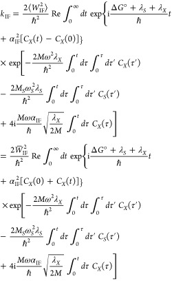10.7

We used the time autocorrelation functions

10.8a

10.8b

for the X and S fluctuations. It was assumed that ⟨δX(t)⟩ = 0, and that the solvent-induced X dependence of ΔH (see eqs 10.1 and 10.5) may be neglected. Moreover, the second-order cumulant expansion was applied to both the static and time-dependent averages involved in eq 10.5 (after insertion of eqs 10.1 and 10.4) under the assumption that the X and ΔH fluctuations are nearly independent Gaussian processes. With these assumptions

10.9

The solvent affects the H transfer rate via two mechanisms: (i) electrostatic interaction with the H transfer system (H species, donor, and acceptor), which appears as a modulation of the free energy of reaction (direct mechanism); (ii) damping of the X vibrational motion that modulates W_IF (indirect mechanism). In fact, the potential for the X oscillator includes an anharmonic term cubic in δX. The model for the X vibrational motion was adapted from prior theoretical models of molecular vibrations in liquids^374−376 and allows X to execute anharmonic vibrations modulated by a stochastic solvent potential.

MD simulations indicate that the time autocorrelation function J_IF(t) vanishes in a few hundredths of a picosecond (see Figure 36), a short time scale compared to that of the solvent response. To explore the relative importance of the direct and indirect mechanisms by which the solvent influences the rate, Borgis and Hynes carried out MD simulations with interactions among the subsystems selectively turned off. As shown in Figure 37, switching off solute–solvent interactions makes J_IF(t) a periodic function with a recurrence time determined by the X vibrational motion (see Figure 37a). The period of the signal is larger than the fundamental frequency of the X harmonic motion because of vibrational anharmonicity. The periodicity of J_IF(t) produces divergence of k in eq 10.5. In fact, this limit does not represent a rate process but rather coherent tunneling back and forth with an oscillating value of the coupling W_IF.

Figure 36.

(a) Time evolution of the flux correlation J_IF (denoted as J in the reported figures) for α_IF = 29 Å^–1 and different solvent reorganization energies: λ_S = 2 kcal/mol (solid line), 8 kcal/mol (dashed line), and 16 kcal/mol (dashed–dotted line). The other model parameters appear in ref (193) (see Figure 20 therein). (b) Time evolution of J_IF for two different values of the X–R coupling parameter α_IF: α_IF = 29 Å^–1 (solid line) and α_IF = 0 (dashed line). A nonzero α_IF enhances J_IF damping, with a significant effect on the reaction rate (see eqs 10.5a and 10.5b). Reprinted with permission from ref (193). Copyright 1993 Elsevier.

Figure 37.

Time evolution of J_IF (denoted as J). (a) Free vibration for a gas-phase solute with an X anharmonic mode. (b) Evolution of J_IF after inclusion of solvent collisional dephasing of the X vibration. The electrostatic interactions with the solvent are not included. (c) All solvent effects are considered. The solvent reorganization energy is extremely small, λ_S = 0.05 kcal/mol, yet J_IF damping is obtained. Reprinted with permission from ref (193). Copyright 1993 Elsevier.

By turning on the dephasing of the X vibrational motion due to the short-range (collisional) interactions with the surrounding solvent molecules, J_IF(t) loses coherence on the picosecond time scale (see Figure 37b), but has a finite asymptotic value that prevents the definition of a rate k. In our view of k as the zero-frequency value of the spectral density of J_IF(t) (see eq 10.5), the nonzero asymptotic J_IF value reflects the fact that introducing only the oscillator dephasing damps the constructive interference responsible for the signal in Figure 37a, but does not remove the zero-frequency coherent component of the reaction. That is, since direct electrostatic interactions between the solvent and the reactive subsystem are switched off, the processes of approaching and leaving the transition region due to solvent fluctuations are not enabled, and the asymptotic J_IF value reflects the nonzero average value of a Rabi-type oscillating transition probability per unit time. The large oscillations in Figure 37a do not appear in Figure 37b, because of the damping of the large X fluctuations and consequent effects on the transition rate.

Including the direct interaction mechanism responsible for the free energy barrier, total incoherence is achieved after the first peak of J_IF(t), as shown in Figures 36 and 37c. The reaction rate can thus be obtained by integration of J_IF(t), as in eq 10.5a.

On the femtosecond time scale of J_IF(t) decay, shown in Figure 37c, the dynamics of the solvent fluctuations (for which the MD simulation gives a correlation decay time of ∼0.1 ps¹⁶⁵) and their effects on the X vibration can be ignored. In this approximation, omitting X damping leads to the time evolution of C_X for an undamped quantum harmonic oscillator:

10.10a

10.10b

Considering only static fluctuations means that the reaction rate arises from an incoherent superposition of H tunneling events associated with an ensemble of double-well potentials that correspond to a statically distributed free energy asymmetry between reactants and products. In other words, this approximation reflects a quasi-static rearrangement of the solvent by means of local fluctuations occurring over an “infinitesimal” time interval. Thus, the exponential decay factor at time t due to solvent fluctuations in the expression of the rate, under stationary thermodynamic conditions, is proportional to

10.11

Substitution of eqs 10.10 and 10.11 into eq 10.7 yields¹⁶⁵

10.12a

with

10.12b

where

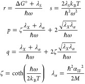10.13

In eq 10.13, λ_α, known as the “coupling reorganization energy”, links the vibronic coupling decay constant to the mass of the vibrating donor–acceptor system. A large mass (inertia) produces a small value of λ_α. Large α_IF values imply strong sensitivity of W_IF to the donor–acceptor separation, which means large dependence of the tunneling barrier on X,¹⁹³ corresponding to large λ_α. The r and s parameters characterize the influence of the solvent on the rate constant; p and q characterize the splitting and coupling features of the X vibration.

The oscillatory nature of the integrand in eq 10.12 lends itself to application of the stationary-phase approximation, thus giving the rate^165,192,193

10.14

where τ_s is the saddle point of Σ_IF in the complex plane defined by the condition Σ_IF′(τ_s) = 0. This expression produces excellent agreement with the numerical integration of eq 10.7. Equations 10.12−10.14 are the main results of BH theory. These equations correspond to the high-temperature (classical) solvent limit. Moreover, eqs 10.9 and 10.10b allow one to write the average squared coupling as^193,228

10.15

Reference (193) shows that eqs 10.12a, 10.12b, 10.13, and 10.14 account for the possibility of different initial vibrational states. In this case, however, the spatial decay factor for the coupling generally depends on the initial, μ, and final, ν, states of H, so that different parameters α_μν and the corresponding coupling reorganization energies (λ_α)_μν appear in k_IF. In addition, one may need to specify a different reaction free energy ΔG_μν° for each μ, ν pair of vibrational (or vibronic, depending on the nature of H) states. Thus, k_IF is written in the more general form

10.16

where the μ → ν rates k_μν are calculated using one of eq 10.7, 10.12, or 10.14, with I = μ, F = ν, and P_μ is the Boltzmann occupation of the μth H vibrational or vibronic state of the reactant species. In the nonadiabatic limit under consideration, all of the appreciably populated H levels are deep enough in the potential wells that they may see approximately the same potential barrier. For example, the simple model of eq 10.4 indicates that this approximation is valid when V ≫ E_μ for all relevant proton levels. When this condition is valid, eqs 10.7, 10.12a, 10.12b, 10.13, and 10.14 can be used, but the ensemble averaging over the reactant states now includes different H vibrational states and their statistical weights. The above formalism, in conjunction with eq 10.16, was demonstrated by Hammes-Schiffer and co-workers to be valid in the more general context of vibronically nonadiabatic EPT.^337,345 They also addressed the computation of the PCET rate parameters in this wider context, where, in contrast to the HAT reaction, the ET and PT processes generally follow different pathways.

Borgis and Hynes also developed a Landau–Zener formulation for PT rate constants, ranging from the weak to the strong proton coupling regime and examining the case of strong coupling of the PT solute to a polar solvent. In the diabatic limit, by introducing the possibility that the proton is in different initial states with Boltzmann populations P_μ, the PT rate is written as in eq 10.16. The authors provide a general expression for the PT matrix element in terms of Laguerre polynomials, yet the same coupling decay constant is used for all couplings W_μν.²²⁸ Note also that eq 10.16, with substitution of eq 10.12, or 10.14, and eq 10.15 yields eq 9.22 as a special case.

10.4. Analytical Rate Constant Expressions in Limiting Regimes

Analytical results for the transition rate were also obtained in several significant limiting regimes. In the high-temperature and/or low-frequency regime with respect to the X mode, ℏω/k_BT ≪ 1, the rate is^192,193,228

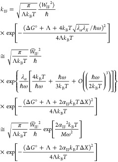10.17

with Λ = λ_S + λ_X + λ_α. In the second expression we used λ_X and λ_α defined in the BH model. The third expression was obtained by Hammes-Schiffer and co-workers^{184,197,337,345} for the sum terms in eq 10.16, under the same conditions of temperature and frequency, using a different coupling decay constant (and hence a different λ_α) for each term in the sum and expressing the vibronic coupling and the other physical quantities that are involved in more general terms suitable for nonadiabatic EPT.

In eq 10.17, the cross-term containing (λ_αλ_X)^1/2 remains finite in the classical limit ℏ → 0 because of the expression for λ_α. This is a consequence of the dynamical correlation between the X coupling and splitting fluctuations, and can be related to the discussion of Figure 33. Application of eq 10.17 to Figure 33 (where S is fixed) establishes that the motion along R (i.e., at fixed nuclear coordinates) is affected by λ_α, the motion along X depends on λ_X, and the motion along oblique lines, such as the dashed ones (which is related to rotation over the R, X plane), is also influenced by (λ_αλ_X)^1/2. The cross-term (λ_αλ_X)^1/2 precludes factoring the rate expression into separate contributions from the two kinds of fluctuations. Regarding eq 10.17, Borgis and Hynes say,¹⁹³ “Note the key feature that the apparent “activation energy” in the exponent in k is governed by the solvent and the Q-vibration; it is not directly related to the barrier height for the proton, since the proton coordinate is not the reaction coordinate.” (Q is X in our notation.) Note, however, that α_IF appears in this effective activation energy. It is not a function of R, but it does depend on the barrier height (see the expression of α_IF resulting from eq 10.4 or the related expression in ref (193), where the barrier top is described as an inverted parabola).

As noted by Borgis and Hynes,^193,228 the non-Arrhenius dependence on the temperature, which arises from the average squared coupling (see eq 10.15), is weak for realistic choices of the physical parameters involved in the rate. Thus, an Arrhenius behavior of the rate constant is obtained for all practical purposes, despite the quantum mechanical nature of the tunneling.

Another significant limiting regime is the opposite of the above, i.e., the low-temperature and/or high-frequency limit defined by ℏω/k_BT ≫ 1. Different cases result from the relative values of the r and s parameters given in eq 10.13. Two such cases have special physical relevance and arise for the conditions λ_S > |ΔG°| and λ_S < |ΔG°|. The first condition corresponds to strong solvation by a highly polar solvent, which establishes a solvent reorganization energy exceeding the difference in the free energy between the initial and final equilibrium states of the H transfer reaction. The second one is satisfied in the (opposite) weak solvation regime. In the first case, eq 10.14 leads to the following approximate expression for the rate:^165,192,193

10.18a

with

10.18b

where

10.18c

The average of the squared coupling is taken over the ground state of the X vibrational mode. In fact, excitation of the X mode is forbidden at temperatures such that k_BT ≪ ℏω and under the condition |ΔG°| < λ_S . (W̅_IF²)_t is defined by eq 10.18c as the value of the squared H coupling at the crossing point X_t = ΔX/2 of the diabatic curves in Figure 32b for the symmetric case. The Condon approximation with respect to X would amount, instead, to replacing ⟨W_IF²⟩₀ with (W̅_IF²)_t, which is generally inappropriate, as discussed above. Equation 10.18a is formally identical to the expression for the pure ET rate constant, after relaxation of the Condon approximation.³³³ Moreover, eq 10.18a yields the Marcus and DKL results, except for the additional explicit expression of the coupling reported in eqs 10.18b and 10.18c. As in the DKL model, the thermal energy k_BT is significantly smaller than ℏω, but much larger than the energy quantum for the solvent motion.

In the limit of weak solvation, λ_S < |ΔG°|^165,192,193

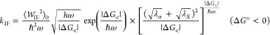10.19a

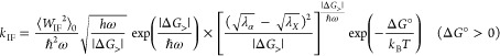10.19b

where |ΔG_<| = ΔG° + λ_S and |ΔG_>| = ΔG° – λ_S. The activation barriers in eqs 10.18a and 10.19 are in agreement with those predicted by Marcus for PT and HAT reactions (cf. eqs 6.12 and 6.14, and also eq 9.15), although only the similarity between eq 10.18a and the Marcus ET rate has been stressed generally in the previous literature.^184,193

Rate constants very similar to those above were elaborated by Suárez and Silbey³⁷⁷ with reference to hydrogen tunneling in condensed media on the basis of a spin-boson Hamiltonian for the HAT system.³⁷⁸

Borgis and Hynes also elaborated an expression for the PT rate constant in the fully (electronically and vibrationally) adiabatic regime, for ℏω/k_BT ≫ 1:

10.20

This rate expression was obtained by Borgis and Hynes²²⁸ as a limiting case of a theoretical treatment encompassing the PT vibrationally nonadiabatic and adiabatic regimes. Equation 10.20 also holds for EPT under the same conditions.¹⁸⁶ As in eq 5.29, ω_S is an effective frequency for solvent motion, and the activation free energy barrier ΔG_act is given by the difference between the values of the ground vibronic level at its maximum and minimum with respect to the solvent collective coordinate (or set of solvent coordinates) S. For ℏω < k_BT, the prefactor is more complicated and depends on ω²²⁸ in a manner consistent with many-body transition-state theory in the frictionless limit.^379−385 This theory can be used, in general, to obtain the rates of transition between the minima corresponding to the four diabatic states of Figure 20,^116,214 and another special case is represented by eq 5.29 for adiabatic ET.

11. Cukier Theory of PCET

In the extended Marcus theory described in section 6, a proton or atom transfer reaction amounts to a bond rupture and formation along internal coordinates (bond distances) that define inner-sphere solute modes of reorganization as in the framework of pure ET. This perspective was adopted in Cukier’s treatment of PCET reactions,¹⁸⁷ which also includes a description of the proton–solvent interaction that is similar to the description of electron–solvent interaction.^116,188

Cukier’s first description of PCET^187,386 reactions was based on the breakdown of the Condon approximation for the electronic coupling with respect to the motion of the transferring protons. The model was motivated by experiments on photoinduced intramolecular ET at nearly fixed distance (in a range typical of nonadiabatic ET) mediated by a hydrogen-bonded interface and characterized by a distinct isotope effect upon deuteration of the proton interface.³⁸⁷ The first proposed model assumed that the ET matrix element, V_IF(R), depended on the proton configuration at the interface, as measured by a coordinate, or a set of coordinates, R. Fermi’s golden rule gives a PCET rate that is proportional to |V_IF(R)|² in the electronically nonadiabatic regime. Thus, the failure of the Condon approximation provides the mechanism for the influence of PT at the hydrogen-bonded interface on the long-distance ET . The effects of the R coordinate on the reorganization energy are not included. The model can lead to isotope effects and temperature dependence of the PCET rate constant beyond those expected for conventional ET. The topology of the class of PCET reaction systems motivating this model is illustrated in Figure 38.

Figure 38.

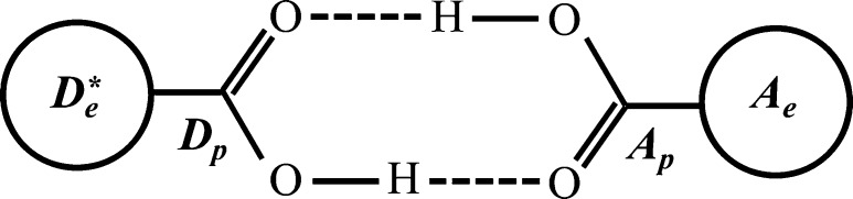
Representative molecular structure for application of the model in eq 11.1 (cf. Figure 1 in ref (187)). A dicarboxylic acid dimer forms the PT interface. Substituents act as the photoexcited electron donor (D_e^*) and electron acceptor (A_e).

The model Hamiltonian of Cukier includes a standard spin-boson representation of ET reactions, and its matrix is expressed, in terms of mass-weighted nuclear coordinates and the Pauli matrices σ̂_x and σ̂_z (the identity matrix is implicitly assumed for the diagonal terms), as^187,388

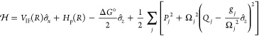11.1

In eq 11.1, V_IF(R) = V₀ exp(−γ|R|) is the ET matrix element, characterized by a decay constant γ and a maximum value of V₀ for the symmetric (transition-state) configuration of the proton(s) described by R = 0.³⁸⁸H_p(R) = T̂_p(R) + V_p(R) is the Hamiltonian associated with the proton, which includes its kinetic energy and the effective proton potential V_p(R). The latter is a double-well potential that corresponds to a hydrogen-bonded proton localized on one or the other side of the PT interface. Q_j, P_j, Ω_j, and g_j are the mass-weighted coordinate, the corresponding momentum, the (angular) frequency and the coupling with the tunneling electron of the jth solvent mode (i.e., an atomic coordinate in a discrete solvent model or a mode of the solvent polarization in a continuum model^116,159,389). The shifts g_j/Ω_j² result from the polaron transformation¹⁴⁹ and the translation operators employed.¹²¹ Nonzero matrix elements of σ̂_z physically reflect expansion of the solvent polarization around the minima of the electronic diabatic surfaces corresponding to the initial (I) and final (F) electronic states. ΔG° is the free energy of reaction. Writing the PCET rate using Fermi’s golden rule, assuming the limit of classical solvent, and a Boltzmann population P_k of the kth proton state in the initial electronic state, Cukier obtained the PCET rate^187,189

11.2

where the vibronic coupling (its modulus needs to be used, in general, for complex wave functions) for the initial and final proton states k and n,³⁹⁰ with vibrational energies ε_k and ε_n, respectively, is

11.3

and the reorganization energy is given, in terms of the solvent frequencies and couplings to the electron donor and acceptor, as^149,343

11.4

Comparing the DKL rate of eq 9.16 with the contribution to the rate in eq 11.2 from the terms that involve the initial proton ground vibrational state, one sees that the differences arise from the fact that the Condon approximation is not used in eq 11.2 for the electronic coupling V_IF and the fact that the harmonic approximation is not assumed a priori for the proton wave functions.

As noted by Cukier,¹¹⁶ the PCET mechanism resulting from the Hamiltonian of eq 11.1 and leading to the rate constant in eq 11.2 applies to cases where the hydrogen-bonded interface is symmetric with respect to the initial and final proton or hydrogen atom localizations. As such, the change in R does not cause significant rearrangement of the interfacial charge distribution (for example, this is expected after hydrogen interchange in the double H-bonded interface of Figure 38 or of compound 2 in Figure 39). This feature also justifies the approximation of the reorganization energy with the solvent contribution λ_S.

Figure 39.

Representative PCET systems relevant to Cukier’s theory. Photoinduced ET takes place from Ru(bpy)₂ to dinitrobenzene. Systems 1 and 3 experience significant charge rearrangement upon PT because of donor–acceptor asymmetry, which implies localization of the proton charge in different environments before and after PCET. The change in charge distribution is sketched in the reaction scheme reported below the compounds. Minor charge rearrangement is expected for PT in 2 following proton interchange, due to the symmetry of the interface. Reprinted from ref (116). Copyright 1995 American Chemical Society.

PCET mechanisms often involve asymmetric hydrogen-bonded interfaces. Examples are reported in Figures 39 and 40. In compounds 1 and 3 of Figure 39, photoexcitation of the Ru(bpy) (bpy =2,2′-bipyridine) electron donor initiates ET to the dinitrobenzene acceptor, which can result in PT at the asymmetrically hydrogen-bonded interface accompanied by large charge redistribution (see the lower panel of Figure 39). A similar PCET motif is envisaged for the Re and Ru complexes in Figure 40, where ET/PT or EPT is active depending on the hydroquinone concentration.

Figure 40.

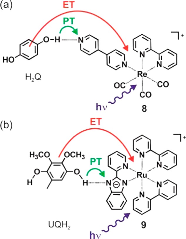
Excited-state PCET systems where the protonatable moiety is the (a) 4,4′-bipyridine or (b) pyridylbenzimidazole ligand. Panel a reprinted from ref (213). Copyright 2013 American Chemical Society. Panel b reprinted with permission from ref (391). Copyright 2011 Wiley-VCH Verlag GmbH & Co. KGaA.

Cukier notes that the sequential ET and PT processes are coupled in the ET/PT mechanism because the effective potential energy for the proton motion is more favorable for PT after the ET event; then separate solvent fluctuations establish resonance conditions for ET and PT.¹¹⁶ Kinetically, ET/PT represents a rate-limited reaction mechanism, since the overall rate constant is approximated by (k_ET^–1 + k_PT^–1)⁻¹ and is thus limited by the slower of the two transfer steps. EPT has the kinetic advantage of not being a rate-limited reaction but also has the kinetic disadvantage that a long tunneling path is required for occurrence of a single tunnel event in the two-dimensional space of electron and proton coordinates. Whether ET/PT or EPT is the favored reaction mechanism can be assessed theoretically by the computation of two kinds of quantities: the coupling matrix elements and the free energies pertaining to solvation of the reactants and products. The latter are the driving force and the reorganization energy contributions to the activation free energy, which depend on the coupling of the solvent polarization to both transferring species. In this regard, Cukier’s model assumes that the PT process is driven by solvent polarization fluctuations in a manner similar to that of solvent coupling to pure ET processes.¹¹⁶

This is the chemical-physical context for most of Cukier’s contribution to PCET theory, focusing on the electronically and vibrationally nonadiabatic PCET regime (e.g., this is the PCET regime expected for the reactions characterized in Table 1 that involve D2-Tyr160, Trp48, and Trp306). The electronically nonadiabatic character of the reaction arises from the distance between the electron donor and acceptor in several PCET systems with a PT interface. The vibrational nonadiabaticity is typical of PT systems that involve intermediate-to-weak hydrogen-bonded systems, which can arise, for example, in rigid intramolecular PT systems, where proton donor–acceptor distances that allow vibrationally adiabatic PT are precluded.^116,392

Cukier devised two different approaches to construct the reaction rate constant, which are described in section 11.1 and allow predictions regarding the dominance of the ET/PT or EPT reaction channel.

11.1. Double-Adiabatic and Two-Dimensional Approaches

The first (double-adiabatic) approach described in this section is related to the extended Marcus theory of PT and HAT, reviewed in section 6, because the transferring proton’s coordinate is treated as an inner-sphere solute mode. The approach is also related to the DKL model interpreted as an EPT model (see section 9).

In Cukier’s PCET model, the reactive electron is coupled to a classical solvent polarization mode and to a quantum internal coordinate describing the reactive proton. Cukier noted that the PCET rate constant can be given the same formal expression as the ET rate constant for an electron coupled to two harmonic nuclear modes. In the coupled ET–PT reaction, the internal nuclear coordinate (i.e., the proton) experiences a double-well potential (e.g., in hydrogen-bonded interfaces). Thus, the energies and wave functions of the transferring proton differ from those of a harmonic nuclear mode. In the diabatic representation appropriate for proton levels significantly below the top of the proton tunneling barrier, harmonic wave functions can be used to describe the localized proton vibrations in each potential well. However, proton wave functions with different peak positions appear in the quantitative description of the reaction rate constant. Moreover, linear combinations of such wave functions are needed to describe proton states of energy near the top of the tunnel barrier. Yet, if the use of the proton state in constructing the PCET rate follows the same formalism as the use of the internal harmonic mode in constructing the ET rate, the PCET and ET rates have the same formal dependence on the electronic and nuclear modes. In this case, the two rates differ only in the physical meaning and quantitative values of the free energies and nuclear wave function overlaps included in the rates, since these physical parameters correspond to ET in one case and to ET–PT in the other case. This observation is at the heart of Cukier’s approach and matches, in spirit, our “ET interpretation” of the DKL rate constant based on the generic character of the DKL reactant and product states (in the original DKL model, PT or HAT is studied, and thus, the initial and final electronic states do not represent donor and acceptor localized electronic states). Thus, the ET theory and the DKL theory for PT are connected in a complementary way with Cukier’s double-adiabatic approach. Compared to the DKL formalism, Cukier’s treatment includes different possible initial states for the proton and uses different methods to arrive at an expression for the rate constant.

Cukier’s analysis begins by considering four coordinates: q (reactive electron), R (reactive proton), Q (solvent mode), and q_i (core electrons). The BO scheme separates the q_i degrees of freedom from the other coordinates and thus removes them from explicit analysis.³⁸⁹ The reduction to a one-electron picture arises from assuming that only the ground multielectron state of the q_i degrees of freedom is populated during the PCET reaction. BO separation of the q coordinate is then used to obtain the initial and final electronic states (from which the electronic coupling V_IF is obtained) and the corresponding energy levels as functions of the nuclear coordinates, which are the diabatic PESs V_I(R,Q) and V_F(R,Q) for the nuclear motion. V_I and V_F are used to construct the model Hamiltonian in the diabatic representation:³⁹³

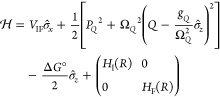11.5

The quantities that refer to the single collective solvent mode involved are defined in eq 11.1 with j = Q. In contrast to the Hamiltonian of eq 11.1, the Condon approximation is used for the electronic coupling. In the Hamiltonian model of eq 11.5 the solvent mode is coupled to both the q and R coordinates. The Hamiltonians H_I(R) = T̂_I^R + V̅_I(R) and H_F(R) = T̂_F + V̅_F(R) express direct coupling between the electron and proton dynamics, because the PES for the proton motion depends on the electronic state in these Hamiltonians. The combination of solvent–proton, solvent–electron, and electron–proton couplings embodied in eq 11.5 allows a more intimate connection to be established between ET and PT than the Hamiltonian model of eq 11.1. In the latter, (i) the same double-well potential V_p(R) corresponds to the initial and final electronic states and (ii) the coupling of electron and proton dynamics is limited to the influence of the R value on the electronic coupling V_IF.

In light of the analysis of section 5.3, the effective potential energies for the proton dynamics in the initial and final electronic states, V̅_I(R) and V̅_F(R), may be interpreted as (i) the averages of the diabatic PESs V̅_I(R,Q) and V̅_F(R,Q) over the Q conformation, (ii) the values of these PESs at the reactant and product equilibrium Q values, or (iii) proton PESs that do not depend directly on Q, i.e., are determined only by the electronic state. The proton PESs V̅_I(R) and V̅_F(R) are referred to as “bond potentials” by Cukier, because they describe the bound proton through the entire R range, for the corresponding electronic states. If the bond potentials are characterized by a large asymmetry (see Figure 41) and depend weakly on the localization of the transferring electron (namely, the dashed and solid lines in Figure 41 are very similar), then no PT occurs: the proton vibrates approximately around the same position in the initial and final ET states. Conversely, very different V̅_I(R) and V̅_F(R) indicate strong coupling of the electron and proton states, as shown in Figure 41.

Figure 41.

Proton PESs that may represent V_I(R,Q) and V_F(R,Q) or V̅_I(R) and V̅_F(R). A strong dependence on the electronic state is illustrated. Before ET (i.e., in electronic state I), the initial proton localization, which is centered on −R₀, is strongly favored compared to its localization after tunneling, i.e., around R₀. The opposite case occurs following ET. Thus, PT is thermodynamically favored to occur after ET. Note that the depicted PESs are qualitatively similar to those in Figure 2 of ref (116) and are comparable with those in Figure 27c.

Based on the above Hamiltonian, and applying standard manipulations of ET theory,^149,343 the PCET rate constant is

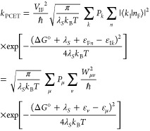11.6a

where

11.6b

The quantum numbers μ = {I,k} and ν = {F,n} are used to distinguish the initial and final proton states, as well as the overall vibronic states. The rate constant is formally similar to that in eq 11.2. However, the rate reflects the critical differences between the Hamiltonians of eqs 11.1 and 11.5. On the one hand, the ET matrix element does not depend on R in eq 11.6. On the other hand, the passage from H_p(R) to {V̅_I(R),V̅_F(R)} leads to different sets of proton vibrational states that correspond to V̅_I(R) and V̅_F(R) (|k_I⟩ and |n_F⟩, respectively).

The harmonic approximation need not be used for the vibrational states in eq 11.6, where, in fact, the initial and final proton energy levels are generically denoted by ε_μ and ε_ν, respectively. Nevertheless, in the derivation of k_PCET, it is assumed that the R and Q Franck–Condon overlaps can be factored.¹¹⁶ Note that eq 11.6 reduces to eq 9.17, obtained within the DKL model, in the harmonic approximation for the vibrational motion of the proton in its initial and final localized states and considering that the proton frequency satisfies the condition ℏω_p > k_BT, so that only the proton vibrational ground state is initially populated. In fact

11.7

The effective potential energy curves in Figure 41 can have up to four minima for given initial and final proton states. Denoting the latter by a and b, respectively, one arrives at the picture in Figure 20 (with state I = state 1 and state F = state 2). The PESs V_I(R,Q) and V_F(R,Q) can be used to evaluate the rate of the proton-coupled ET in eq 11.6 and the PT rate constants k_ab^I,F for a fixed electron state. As noted in ref (116), this can be done by invoking the double-adiabatic approximation, as proposed in the DKL model.^178−180 Solving the Schrödinger equation for proton motion at fixed Q yields the four diabatic states in Figure 20 in the form of BO electron–proton wave functions (see section 5.3), ψ_jn(q,R,Q) = ϕ_j(q;R,Q)χ_n(R;Q),³⁹⁴ and the respective effective potentials in the BO approach, V_a,b^I,F(Q), which determine the dynamics of the solvent polarization. The proton wave functions can be used to compute PT matrix elements. The PESs V_a,b(Q) or V_a,b^F(Q) yield the reaction free energy and reorganization energy for pure PT while the system is in the I or F electronic state. These PESs can be approximated as harmonic polarization surfaces with origins specific to the electron–proton states, thus leading to PT rate constants k_ab and k_ab^F that have the standard one-mode golden rule form.

In summary, the double-adiabatic separation scheme provides electronic couplings and free energy parameters required to compute the PCET and the PT rate constants for each state of the transferring electron. As noted by Cukier,¹¹⁶ eq 11.6 describes either PCET or pure ET, depending on the proton displacement that accompanies ET.³⁹⁵ If ET occurs first, the PT process that follows the ET event depends on the final electronic state. However, the concerted nature of the reaction is better captured by a method that treats the electron and proton on an equal footing, rather than a method based on double-adiabatic separation, which creates a privileged role for the first separated electronic degree of freedom. This consideration motivated Cukier’s two-dimensional formulation, where the PCET mechanism is described with a two-dimensional PES that is parametric in the solvent coordinate:¹¹⁶

11.8

V_e is the effective PES for the isolated transferring electron. V_e is a symmetric double-well potential, with minima at −q₀ and q₀ for the I and F electronic states, respectively. Similarly, V_p is a symmetric potential for the isolated PT system, with minima at −R₀ and R₀ for the a and b proton states, respectively. The electron–proton coupling γ determines the effects of one reaction on the other one. γ is the electron–proton coupling strength. In Cukier’s perspective,¹¹⁶ where ET/PT and EPT are the two processes of interest, the γ term in eq 11.8 describes the change in electronic structure associated with the ET reaction that favors the PT event (ET/PT mechanism; see Figure 41) or the coupling of the ET and PT events (concerted reaction mechanism). Whether the γ coupling promotes PT following ET or EPT also depends on the solvation energetics. The c_e (c_p) term provides the coupling of the electron (proton) charge with the solvent polarization.

In this two-dimensional perspective, the transferring electron and proton are treated in the same fashion, “as quantum objects in a two-dimensional tunneling space”,¹⁸⁸ with one coordinate that describes the electron tunneling and another that describes proton tunneling. All of the quantities needed to describe ET, PT, ET/PT, and EPT are obtained from the model PES in eq 11.8. For example, when the proton is at its initial equilibrium position −R₀, the ET reaction requires solvent fluctuations to a transition-state coordinate Q_ta where −γqR + c_eqQ = 0, i.e., Q_ta = −γR₀/c_e. At the position (−q₀,–R₀,Q_ta), we have ∂V(q,R,Q) ∂q = 0. Thus, the reactive electron is at a local minimum of the potential energy surface, and the potential double well along q (which is obtained as a profile of the PES in eq 11.8 or is a PFES resulting from a thermodynamic average) is symmetric with respect to the initial and final diabatic electron states, with V(−q₀,–R₀,Q_ta) = V(q₀,–R₀,Q_ta) = V_e(q₀) + V_p(−R₀) + γR₀²c_p/c_e (see Figure 42). Using the language of section 5, the solution of the electronic Schrödinger equation (which amounts to using the BO adiabatic separation) for R = −R₀

11.9

yields the minimum electronic energy level splitting in Figure 42b and consequently the ET matrix element as |V_s(−R₀,Q_t) – V_a(−R₀,Q_t)|/2. Then use of eq 5.63 in the nonadiabatic ET regime studied by Cukier gives the diabatic PESs V_I,F(R,Q) for the nuclear motion. These PESs (or the corresponding PFESs) can be represented as in Figure 18a. The free energy of reaction and the reorganization energy for the pure ET process (and hence the ET activation energy) are obtained after evaluation of V_I,F(R,Q) at Q_t and at the equilibrium polarizations of the solvent in the initial (Q_I0) and final (Q_F0) diabatic electronic states, while the proton is in its initial state. The procedure outlined produces the parameters needed to evaluate the rate constant for the ET_a step in the scheme of Figure 20. For a PT/ET reaction mechanism, one can similarly treat the ET_b process in Figure 20, with the proton in its final state. The PT/ET reaction is not considered in Cukier’s treatment, because he focused on photoinduced reactions.¹⁸⁸

Figure 42.

Effective potential energies (free energies) for the electronic motion at the initial equilibrium (Q_I), transition-state (Q_t), and final equilibrium (Q_F) solvent configurations, when the proton is in the initial state (with average position −R₀). The electronic coupling V_IF is also indicated (cf. Figure 3 in ref (116)).

The same considerations apply to the computation of the PT rate, after interchange of the roles of the electron and the proton. Moreover, a two-dimensional Schrödinger equation can be solved, at fixed Q, thus applying the BO adiabatic separation to the reactive electron–proton subsystem to obtain the electron–proton states and energies relevant to the EPT reaction.

Considering the different time scales for electron and proton motion, the symmetry with respect to the electron and proton is broken in Cukier’s treatment, producing a substantial simplification. This is accomplished by assuming a parametric dependence of the electronic state on the proton coordinate, which produces the “zigzag” reaction path in Figure 43. The proton moves (electronically) adiabatically, with the electron in its initial localized state, to the transition-state coordinate R_t for electron tunneling. At R = R_t, the electronic dynamics is governed by a symmetric double-well potential and the electron tunneling occurs with a transition probability proportional to the square of the electronic coupling between the I and F states. The proton relaxes to its final state after ET. Using the model PES in eq 11.8, the transition-state coordinates of the proton, R_t, and the solvent, Q_t, are related by¹¹⁶

11.10

Equation 11.10 provides a constraint on the transition-state nuclear coordinates. Another relationship between R_t and Q_t is obtained by applying the principle of energy conservation to the overall reaction. Assuming, for simplicity, that the c_p coupling term can be neglected in the tunneling analysis (even if it is not neglected in calculating the activation energy),¹¹⁶ one obtains V(−q₀,–R_t,Q_t) – V(q₀,R_t,Q_t) = −2c_eq₀Q_t. Then, if the initial and final potential wells experienced by the transferring proton are approximately harmonic, the conservation of energy gives −2c_eq₀Q_t + ℏω_p/2 = (n + 1/2)ℏω_p (see Figure 44), that is

11.11

Equations 11.10 and 11.11 exemplify the determination of R_t and Q_t with the above approximations. The actual evaluation of R_t and Q_t requires a model for the coupling of the electron to the solvent (c_e). Moreover, despite the above simplification, c_p also needs, in general, to be estimated. c_e and c_p lead to different Q_t values for ET, PT, and EPT, since Q_t depends on the molecular charge distributions in the initial and final states of the electron and proton. A continuum electrostatic model was used by Cukier to evaluate the solvation energetics, as described in the next section.

Figure 44.

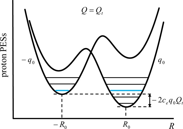
PESs and proton levels at the transition-state solvent configuration Q_t for different electronic states: the initial state, with average electronic coordinate −q₀, and the final one, with average electron coordinate q₀. The two lowest proton vibrational levels that allow energy conservation, given by −2c_eq₀Q_t + ℏω_p/2 = (n + 1/2)ℏω_p, are marked in blue (after Figure 5 of ref (116)).

Cukier argued that, if the c_p coupling is not neglected in the tunneling analysis, each proton level in Figure 44 carries an intrinsic dependence on Q, although “this additional Q dependence should be slight” ¹¹⁶ in asymmetric double-well effective potentials for the proton motion such as those in Figure 44. The term c_pRQ arises from a second-order expansion of the interaction between the solvent and the reactive solute. The magnitude of this coupling was accurately estimated in the DKL model for PT reactions, using the dielectric continuum approximation for the solvent and taking into account the large difference between typical proton and solvent vibrational frequencies.¹⁷⁹ By applying the DKL analysis to the present context, one can see that the coupling c_pRQ can be neglected for nuclear displacements around the equilibrium coordinates of each diabatic electronic PES involved in the Cukier model, which supports the Cukier argument reported above.

The picture that emerges from Figures 43 and 44 allows evaluation of the vibronic coupling for the concerted PCET reaction in the fully (electronically and vibrationally) nonadiabatic regime. The necessary initial and final proton wave functions are obtained for the one-dimensional effective potentials of Figure 44. With the above approximations, these wave functions do not depend on Q_t, which in the vibrationally nonadiabatic limit determines only the shift of one potential well with respect to the other one. Regarding the electronic component of the vibronic coupling (i.e., the electronic coupling V_IF), the zigzag reaction path of Figure 43 indicates that V_IF should be computed at the transition state from the potential V_e(q), as for pure ET. Using these ingredients, the vibronic coupling in Cukier’s “two-dimensional method” is given again by eq 11.6b. Cukier also provided an analytical derivation of eq 11.6b that is based on the BO separation of the electron and proton motion and follows a methodology developed to treat vibration-assisted proton tunneling.^396−398 In the analogy used to apply this methodology, the proton and the low-frequency vibrational mode are replaced by an electron and a proton, respectively. Once this correspondence is established, the procedure developed for vibration-assisted tunneling can be applied, even if the initial and final states of the low-frequency mode do not correspond to a tunneling event, while in the PCET context both the electron and the proton tunnel. Using the golden rule formulation of the PCET rate constant and eq 11.6b, k_PCET is expressed by eq 11.6a, as in the double-adiabatic approach. Thus, the two-dimensional approach is reduced to the double-adiabatic method by using eq 11.6b.^116,188

11.2. Reorganization and Solvation Free Energy in ET, PT, and EPT

The free energy parameters in eqs 11.6 and 11.7 are computed using continuum electrostatic models. The reaction free energy ΔG° contains electronic structure (ΔE^el) and solvation (ΔG^solv) contributions. ΔE^el arises from the difference in electronic structure of the gas-phase solute system in the initial and final electronic states. ΔG^solv is the difference in solvation free energy between the reactant and product states resulting from the coupling of the transferring electron and proton to the solvent or, in more general terms, to the environment of the reaction. ΔG^solv depends on the proton coordinate and on the solvent polarization field, whose fluctuations are critical for reaching the transition state. The polarization correlation functions and the dielectric permittivity describe the nuclear configurational fluctuations in a continuum approximation. In ET reactions, the donor-to-acceptor electron motion is slow compared to the solvent electron motion¹⁵⁹ and very fast with respect to nuclear polarization. This distinction in time scales distinguishes between “inertialess” polarization, approximately identified with the electronic polarization (resulting from the electronic motion in response to the external solute field), and “inertial” polarization, i.e., the nuclear polarization (accompanied by the electronic polarization induced by the nuclear motion). Aside from possible refinement of this distinction,³⁹⁹ its application to PCET may be subtle because the time scale of the proton motion, compared to that of the electron motion, is closer to the time scale range of the solvent dynamics.¹⁵⁹ However, the described distinction between inertial and intertialess polarization can still be a good approximation in many cases (e.g., for solvent and proton frequencies in the DKL model) and can support Cukier’s model, where proton and electron motion are similarly (even though not identically) coupled to the solvent dynamics. However, the significance of treating the fast solvent electronic polarization quantum mechanically to compute the correct activation free energies and transition states was described in earlier studies of ET systems (Gehlen et al.,⁴⁰⁰ Kim and Hynes⁴⁰¹), and such approaches are relevant to PCET reactions as well.

The Hamiltonian leading to the rate constant in eq 11.6 does not include the displacement of the solvent equilibrium position in response to the proton position R. This approximation implies asymmetry in the treatment of the electron and proton couplings to the solvent (which also affects the application of the energy conservation principle to the charge transfer mechanism). However, Cukier showed that this approximation can be relaxed, while still obtaining the PCET rate constant in the form of eq 11.6, by suitably incorporating the proton–solvent coupling in the rate free energy parameters.¹⁸⁸ Here, we summarize the conclusions of Cukier, referring to the original study for details.¹⁸⁸ Using the pioneering polaron theory of Pekar,^402,403 Marcus ET theory,^147,148 and subsequent developments,^{217,401,404−409} Cukier obtained the following expression for the initial diabatic free energy as a function of the proton coordinate and solvent polarization:

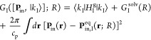11.12a

where the equilibrium orientational polarization field corresponds to the electric displacement field D_I= (4π/c_p)P_in,I^eq and

11.12b

is the equilibrium (Born) solvation energy for the solute with the proton at R and the electron on the donor. H_I^g is the diagonal element of the gas-phase solute Hamiltonian H^g with respect to the initial localized electronic state:

11.12c

E_I^el includes the electronic kinetic energy and, for a potential energy as in eq 5.4, the part of the potential energy that is independent of the proton coordinate. Although E_I,F depend on R (through the parametric dependence of the electronic state), this R dependence is neglected.

Simplification is achieved by assuming that ΔE^el = E_F^el – E_I is not sensitive to the proton state, so that ΔE^el does not depend on whether ET occurs as part of an ET/PT or concerted ET–PT reaction mechanism. Analogous expressions hold for the free energy surface corresponding to the final electronic state. In eq 11.12,c_p is the Pekar factor

11.13

where ε_s and ε_∞ are the static and optical dielectric constants, respectively. D_I² is the R-dependent squared modulus of the electric displacement field D(r) in the solvent in the initial electronic state. P_in(r) is the inertial (orientational) polarization field, and P_in,I^eq(r;R) is its equilibrium value with the proton at R and the transferring electron in its initial localized state. In the first term of eq 11.12a, the proton is treated as a quantum particle, and a functional dependence of the free energy on the proton wave function appears. In the other two terms of eq 11.12a, the electron and proton squared wave functions are inserted as “static” clouds of negative and positive charge surrounding the positions q and R, respectively

11.14

11.15

(where e is the magnitude of the electron charge), and analogous expressions are used for the final electronic state. The fraction f_α ^I of electron charge located at r_α does not depend on q. This expresses the fact that the localized electronic wave function is insensitive to changes in the nuclear coordinates. The fraction f_β of proton charge at r_β depends on the position R. This is an expression of the fact that, as the proton moves along the hydrogen bond, the polarization changes accordingly and affects the proton charge distribution. Using, in eq 11.15, charge sites at fixed positions with charges that depend on the proton location is a convenient way to produce the proton–solvent coupling.¹¹⁶ As a consequence of the f_β ^I dependence on R, the electric displacement field generated by the proton depends on R. This causes an explicit dependence of the diabatic free energy surfaces on the proton position R. Since, in the model, the electron and the proton behave as external (prescribed) sources of electrostatic fields and the dielectric image effects related to the presence of solute–solvent interfaces are neglected, the electronic polarization and the orientational polarization are longitudinal fields.^159,405 Moreover, the orientational polarization shows a parametric dependence on R, owing to the large difference between the typical frequencies of the proton motion and the dynamics of the solvent inertial polarization.

The last term in eq 11.12a represents the fluctuations of the orientational polarization away from its equilibrium value (which depends on the electronic state and on R) that can drive the system to the transition state. Ultimately, the diabatic free energy surfaces have a functional dependence on the solvent polarization and on the proton wave function (gas-phase term), as well as an explicit dependence on R, which is a consequence of the approximation made in treating the proton as a given charge distribution coupled to the solvent polarization (thus precluding the self-consistent determination of its wave function and the polarization driving the charge transfer). This approximation can be good, and it allows evaluation of the effects of solvation on the effective PESs for the proton motion in each electronic state. The solvated PESs contain the gas-phase potential energy, V_I^g(R), and the equilibrium solvation free energy, G_I(R), so the proton wave functions and energies required to obtain the rate constants (e.g., see eq 11.6, where the proton wave functions determine the Franck–Condon factors and the proton energy levels influence the activation energy) are derived from the Schrödinger equation

11.16

and the corresponding Schrödinger equation for the final electronic state. The dependence of the equilibrium inertial polarization field, and therefore of the electric displacement field, on the proton coordinate, as well as the Q-dependent electronic solvation, affects the proton vibrational states obtained from eq 11.16 through G_I^solv(R). This solvation “effective potential” introduces the intrinsic dependence of the proton levels in Figure 44 on a solvent reaction coordinate Q. Such a coordinate is not introduced in ref (188) but can be elicited from eq 11.12. Without resorting to derivations developed in the context of ET,²¹⁷ one may consider that, as for pure ET^216,222,410 (see also section 5.3), the energy gap between diabatic free energy surfaces in eq 11.12 measures the departure from the transition-state coordinate for the PCET reaction. Hence, a reaction coordinate Q may be defined as the part of the diabatic free energy difference that depends on the fluctuating polarization field P_in(r) and thus changes during the reaction, leading to the transition-state coordinate Q_t:^217,222

11.17

where the initial and final localized proton states are characterized by coordinate values R_a and R_b, respectively. In particular, at Q_t we have P_in,I^eq = P_in,F, which gives G_I = G_F. In the EPT reaction mechanism, the same solvent coordinate fluctuation enables both proton and electron tunneling. Thus, eq 11.17 defines the reaction coordinate. However, for other concerted reaction mechanisms, the proton and electron pathways are generally different, and the overall solvent fluctuations may be better characterized in terms of components directly associated with the ET and PT events. Moreover, the two-dimensional mechanism illustrated in Figure 43, while describing concerted tunneling, still generates distinct one-dimensional paths for electron and proton tunneling. These considerations indicate that, in general, it is useful to define more than one reaction coordinate. This issue is tackled in the next section.

In addition to the proton quantities derived from eq 11.16, the other two ingredients that need to be inserted into eqs 11.6a and 11.6b are obtained from eq 11.12. The solvent reorganization free energy for the PCET reaction is computed as the change in G_I between the equilibrium inertial polarization fields corresponding to the initial and final solute states, but with the solute in the initial state:

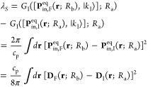11.18

The reaction free energy is given by

11.19

While the equilibrium displacement of the solvent can change appreciably as the center of the proton wave function moves from R_a to R_b, if the proton remains in the left potential well of Figure 44, and thus only ET occurs, the equilibrium displacement of the solvent can be assumed independent of the proton position around R_a. In this event, if the proton degree of freedom can be treated as a quantum mechanical normal mode of vibration, while P_in is a classical mode, only R_a appears in the above equations and eq 11.6 reduces to a well-known rate constant expression for nonadiabatic ET.^186,343,389

After insertion of eqs 11.14, 11.15, 11.18, and 11.19 into eqs 11.6a and 11.6b, evaluating the rate constant requires quantum chemical investigation of the gas-phase contribution in eq 11.12 and a specific model to compute the solvation free energy of the reactive system, as a function of the proton coordinate, for each diabatic electronic state. The latter is in the focus of Cukier’s analysis^116,188,189 and is defined by an ellipsoid of revolution with four charge sites shown in Figure 45, with particular relevance to PCET systems such as those of Figures 39 and 40.

Figure 45.

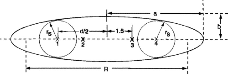
Ellipsoidal model adopted by Cukier for evaluating the reorganization and solvation free energies of the ET, PT, and EPT processes. The electron donor and acceptor are modeled as spheres of radius r_s, centered at points 1 and 4, embedded in a solvent continuum. The latter is described as an ellipsoid with major (minor) axis a (b) and interfocal distance R (R denotes the proton coordinate elsewhere in this review). The distance d between sites 1 and 4 is fixed at 15 Å. The proton donor and acceptor are located at points 2 and 3, 3 Å apart. Reprinted from ref (116). Copyright 1995 American Chemical Society.

In Figure 45, points 1 and 4 are the centers of the electron donor and acceptor and are taken at a distance d = 15 Å. The electron donor and acceptor are modeled as spheres of radius r_s of 3–4 Å embedded in an ellipsoid with major (minor) axis a (b) and interfocal distance R. The ellipsoid contains the donor and acceptor groups (the ellipsoid and the spheres of radius r_s are tangent to each other). Points 2 and 3 mark the sites at the PT interface used to describe the proton charge distribution along the hydrogen bond involved in the reaction. Cukier obtains ΔG^solv and λ_S from this continuum model by employing expressions obtained by Kirkwood and Westheimer^411,412 and by Ehrenson, Brunschwig, and Sutin, respectively.^413,414 Details can be found in refs (116), (188), and (189).

The solvation energetics decreases with increasing ellipsoid size due to overall weakening of the electrostatic interactions with the solvent. Moreover, λ_S turns out to be smaller for PT than for ET and PCET, which “reflects the dipole character of the relatively close proton charge sites”.¹¹⁶ In fact, the proximity of the proton donor and acceptor exposes the acceptor to the polarization field induced by the donor. This suggests that the solvent polarization before PT is already partly adjusted to the charge distribution of the products, with less environmental reorganization required by the PT reaction. The same argument applies to the comparison between ET systems with diverse donor–acceptor distances⁴¹⁵ as expected from Marcus’ expression for the reorganization energy.⁷

Evaluation of rate constants for concerted PCET is simplified by the assumption that the proton–solvent interaction is similar for proton quantum states localized in the same potential well. This assumption is justified by the localization of the proton wave functions on the length scales of the solutes and allows use of the same set of charges in eq 11.15 for all proton states localized around R_a and for those localized around R_b.

Cukier’s analysis was applied to distinguish between ET/PT and EPT mechanisms. In this regard, Cukier noted¹¹⁶ that, on the one hand, EPT is disadvantaged compared to ET/PT by a long tunnel path for the concerted ET–PT event and, on the other hand, the concerted occurrence of ET and PT in the EPT mechanism allows population of vibrational levels corresponding to smaller activation energy compared to that of ET/PT. For example, the ET/PT pathway is unlikely if the solvation energetics brings about strongly endergonic ET, even if the PT step is fast, since the overall rate constant (k_ET^–1 + k_PT^–1)⁻¹ would be limited by k_ET.

11.3. Generalization of the Theory and Connections between PT, PCET, and HAT

Cukier’s theoretical treatment of PCET was later extended to the electronically adiabatic and vibrationally nonadiabatic-to-adiabatic regimes, using a Landau–Zener model.¹⁹⁰ A motivation—and one of the main purposes of this extension—was to describe HAT, which is characterized by (a) electron tunneling through relatively short distances, such that electronic adiabaticity is expected throughout the reaction, and (b) smaller charge rearrangement and weaker coupling to the solvent medium than in ET, PT, and PCET reactions, because of the neutrality of the transferring particle. The description of HAT rests on a previous treatment of PT ranging from the nonadiabatic to the adiabatic regime.⁴¹⁶ Cukier’s analysis begins with nonadiabatic PT. It is assumed that the electronic structure changes accompanying the PT event significantly shift the proton stability, similarly to what is represented in Figure 41 for cases where ET is also at play. The electronic solvation helps proton stabilization at all values of the solvent coordinate, thus contributing to creation of the PES minima in Figure 46. This stabilization reduces the proton coupling compared to that in the gas-phase solute and can also lead to situations where the ground vibrational states in the initial and final proton wells dominate the PT reaction.

Figure 46.

Effective potential energies for the proton wave function at the initial equilibrium (Q_i), transition-state (Q_t), and final equilibrium (Q_f) solvent configurations. V_if^p is the proton coupling, which is half the splitting of the symmetric and antisymmetric adiabatic proton states resulting from a double-adiabatic approximation (see ref (416) from which this figure is inspired).

The shape of the effective potential experienced by the proton also depends strongly on the inertial polarization and, in particular, on the value of coordinate (or set of coordinates) X that describes the close nuclear framework of the reaction and is often taken as the proton donor–acceptor distance. Moreover, because of charge displacement accompanying the X motion, the electronic solvation also significantly affects the potential felt by the X degree of freedom. The proton or hydrogen atom tunneling barrier, and hence the nonadiabatic or adiabatic behavior of the transfer reaction, depends strongly on the range explored by the non-Condon coordinate X. Thus, X is a crucial quantity for theories that span from the vibrationally nonadiabatic to the adiabatic regime. Typical frequencies of X motion in the range of 200–250 cm^–1 justify its quantum mechanical treatment, but the comparable value of k_BT/ℏ implies that several states of the X mode contribute to the PT rate, thus providing a number of channels for the transfer.

On the basis of these considerations, and using the golden rule, the rate constant for nonadiabatic PT is^190,416

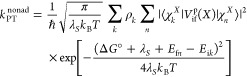11.20

where i (f) denotes the initial (final) localized proton state, k (n) runs over the states |χ_k^X⟩ (|χ_n⟩) of the X degree of freedom in the initial (final) proton state, ρ_k is the occupation probability of state |χ_k^X⟩, E_ik (E_fn) is the energy eigenvalue associated with |χ_k⟩ (|χ_n^X⟩), and V_if(X) is the proton coupling that, exploiting the WKB approximation, is written as^190,417

11.21

The PT rate constant in the adiabatic limit, under the assumption that only two proton states are involved, is

11.22

Cukier arrived at an expression for the rate constant that is valid from the nonadiabatic to the adiabatic regime, by exploiting the Landau^154,155–Zener^156,157 formalism familiar in the context of ET reactions^190,416 and used later in the context of PT reactions.^356,418 The “PT Landau–Zener” parameter is

11.23

where ω_S is a characteristic solvent frequency,^356,419 and the rate constant is⁴¹⁶

11.24a

where

11.24b

The first factor in eq 11.24b may be compared with eq 5.28, and the second interpolating factor is required to obtain the correct limiting forms of eqs 11.20 and 11.22.

In the case of EPT or HAT, the ET event can be accompanied by vibrational excitation. As a consequence, analysis similar to that leading to eqs 11.20–11.22 provides a rate constant with multiple summations: two sums on proton states of eq 11.6 and two sums per each pair of proton states as in eq 11.20 or 11.22. The rate expression reduces to a double sum if the proton states involved in the process are again restricted to a single pair, such as the ground diabatic proton states whose linear combinations give the adiabatic states with split levels, as in Figure 46. Then the analogue of eq 11.20 for HAT is¹⁹⁰

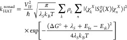11.25

where the values for the free energy parameters also include transfer of an electron. Equations 11.20 and 11.25 have the same structure. The similarity of k_PT and k_HAT is also preserved in the adiabatic limit, where the vibronic coupling does not appear in the rate. This observation led Cukier to use a Landau–Zener formalism to obtain, similarly to k_PT, an expression for k_HAT that links the vibrationally nonadiabatic and adiabatic regimes. Moreover, some physical features of HAT reactions (similar hydrogen bond strengths, and hence PESs, for the reactant and product states, minimal displacement of the equilibrium values of X before and after the reaction, low characteristic frequency of the X motion) allow k_HAT to have a simpler and clearer form than k_PT. As a consequence of these features, a small or negligible reorganization energy is associated with the X degree of freedom. The final expression of the HAT rate constant is¹⁹⁰

11.26

where P(X) is the thermally averaged X probability density, L = H (protium) or D (deuterium), and A_if(X) is given by eq 11.24b with u_if^kn defined by

11.27

The notation in eq 11.26 emphasizes that only the rate constant in brackets depends appreciably on X. The vibrational adiabaticity of the HAT reaction, which depends on the value of u_if(X), determines the vibronic adiabaticity, while electronic adiabaticity is assured by the short charge transfer distances. k_HAT^L depends critically on the decay of S_if with donor–acceptor separation. The interplay between P(X) and the distance dependence of S_if^p leads to a variety of isotope effects (see ref (190) for details).

Cukier’s treatment of HAT reactions is simplified by using the approximation that only the ground diabatic proton states are involved in the reaction. Moreover, the adiabaticity of the electronic charge transition is assumed from the outset, thereby neglecting to consider its dependence on the relative time scales of ET and PT. We will see in the next section that such assumptions are overcome in the theoretical framework of Hammes-Schiffer and co-workers.

12. Soudackov–Hammes-Schiffer (SHS) Theory of PCET

Hammes-Schiffer and co-workers presented a unified theoretical framework to describe sequential and concerted electron–proton transfer reactions, including HAT as a special case of simultaneous ET and PT between the same donor and acceptor groups. In the SHS theory, Cukier’s treatment was extended and generalized by introducing two collective solvent coordinates corresponding to ET and PT, within the formalism of the multistate continuum theory applied to multiple charge transfer reactions.^191,214,420 Dynamical effects of the solvent and of the proton donor–acceptor distance were included in SHS analysis^{225,337,345,421} using the formalism of Borgis and Hynes^192,165 in conjunction with expressions for the diabatic free energy difference and the coupling appropriate for the general context of PCET (where pairs of electron–proton surfaces corresponding to different electronic states are involved in the charge transitions).³³⁷ Hammes-Schiffer’s work also led to a comprehensive classification of PCET reactions^182,215 in terms of time scales, couplings, and theoretical methods that are applicable to the different PCET regimes. This classification of PCET reactions is of great value, because it can assist in directing theoretical-computational simulations and the analysis of experimental data.

12.1. Regarding System Coordinates and Interactions: Hamiltonians and Free Energies

The SHS treatment of PCET reactions is developed with special attention to the definition and quantitative evaluation of the relevant coordinates and their states. This approach provides a route to address the complexities of the PCET mechanisms that arise from the wide range of time scales and of “special” degrees of freedom at play, compared to the case for separate ET and PT. It is in this perspective that multistate continuum models^{193,217,336,389,422} offer some important advantages over atomistic models for PCET reactions: (a) they enable a clear physical picture of the reaction mechanism at low computational cost; (b) the solvent electronic polarization can be consistently included in the model;^401,423 (c) charge transfer reactions can be described in terms of an arbitrary number of basis states. One cannot demand detailed dynamical information from such models. This information is provided at a much higher computational cost from QM/MM approaches.^262,322,424 Hammes-Schiffer and co-workers used a multistate continuum theory³³⁶ in part of their theoretical treatment of PCET by developing the formalism for direct application.^191,214,420 In the theory, the solvent is described as a dielectric continuum and the solute is described using a multistate valence bond (VB) model. The quantum mechanical degrees of freedom corresponding to the transferring proton and electron, and to the other active electrons in the ET and PT subsystems, are treated explicitly. Active electron orbitals are placed on the electron donor (ζ_De) and acceptor (ζ_Ae), on the proton donor (ζ_Dp) and acceptor (ζ_Ap), and on the transferring H species (ζ_H). In terms of the occupations of these orbitals, the four VB states in eq 5.38 are described by the following electronic wave functions²¹⁴ (state 1 ≡ state I and state 2 ≡ state F in the notation used here):

12.1a

12.1b

12.1c

12.1d

where |0⟩ represents the vacuum state with respect to the electron active space, α and β denote spin components (or functions), and the usual creation operator notation is used. In eq 12.1a, the first creation operator builds the excess electron charge on the electron donor; the spin singlet represents the two-electron bonding wave function for the proton donor, D_p, and the attached proton; and the last two creation operators generate the lone pair on the proton acceptor A_p in the initial localized proton state. Equations 12.1b–12.1d are interpreted in a similar manner.

The model of PCET in eqs 12.1b–12.1d can be further reduced to two VB states, depending on the nature of the reaction. This is the case for PCET reactions with electronically adiabatic PT (see section 5).^191,194 Moreover, in many cases, the electronic level separation in each diabatic electronic PES is such that the two-state approximation applies to the ET reaction. In contrast, manifolds of proton vibrational states are often involved in a PCET reaction mechanism. Thus, in general, each vertex in Figure 20 corresponds to a class of localized electron–proton states. Ab initio methods can be used to compute the electronic structure of the reactive solutes, including the electronic orbitals in eq 12.1 (e.g., time-dependent density functional theory has been used very recently to investigate excited state PCET in base pairs from damaged DNA⁴²⁵).

The off-diagonal (one-electron) densities arising from eq 12.1 are

12.2

(these quantities arise from the electron charge density, which carries a minus sign; see eq 4 in ref (214)). The nonzero terms in eq 12.2 typically can be neglected due to the small overlap between electronic wave functions localized on the donor and acceptor. This simplifies the SHS analysis but also allows the classical rate picture, where the four states (or classes of states) represented by the vertices of the square in Figure 20 are characterized by occupation probabilities and are kinetically related by rate constants for the distinct transition routes in Figure 20. The differences between the nonzero diagonal densities ρ_Ia,Ia, ρ_Ib,Ib, ρ_Fa,Fa, and ρ_Fb,Fb give the changes in charge distribution for the pertinent reactions, which are involved in the definition of the reaction coordinates as seen in eq 11.17. Two independent collective solvent coordinates, of the type described in eq 11.17,^217,222 are introduced in SHS theory:

12.3a

12.3b

The second formulation of each reaction coordinate in eq 12.3 is obtained by inserting the expression for the electrostatic potential field generated by the inertial polarization field and then the vacuum electrostatic fields created by the charge densities, i.e.

12.4

While in Cukier’s model the electric displacement fields depend on the proton position (i.e., in a quantum mechanical description of the proton, on the center of its wave function distribution), in the above equations they depend on the proton state. Equations 12.3a (12.3b) define Q_p (Q_e) as the difference in the interaction energies of the two VB states involved in the PT (ET) reaction with the inertial polarization of the solvation medium. Thus, the dynamical variables Q_p and Q_e, which describe the evolution of the reactive system due to solvent fluctuations, are defined with respect to the interaction between the same initial solute charge density ρ_Ia,Ia and P_in. In the framework of the multistate continuum theory, such definitions amount to elimination of the dynamical variable corresponding to ρ_Ia,Ia. Indeed, once Q_p and Q_e are introduced, the dynamical variable corresponding to ρ_Fb,Fb – ρ_Ia,Ia, Q_pe (the analogue of eq 11.17 in SHS treatment), can be expressed in terms of Q_p and Q_e and thus eliminated. In fact

12.5

(the last equality arises from the fact that ρ_Fb,Fb – ρ_Ib,Ib = ρ_Fa,Fa – ρ_Ia,Ia according to eq 12.1); hence

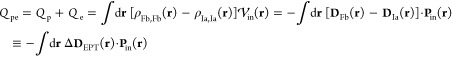12.6

In the classical rate picture arising from the assumption of zero off-diagonal density matrix elements, eq 12.6 is understood to arise from the fact that the EPT and ET_a/PT₂ or PT₁/ET_b reactions illustrated in Figure 20 correspond to the same initial and final states. The two independent solvent coordinates Q_p and Q_e depend on the VB electronic structures determined by different localization characteristics of the electron and proton, but do not show an explicit (parametric) dependence on the (instantaneous) proton position. Similarly, the reaction coordinate of eq 11.17 involves only the average initial and final proton positions R_a and R_b, which reflect the initial and final proton-state localization. In both cases, the usually weak dependence of the solvent collective coordinate(s) on local proton displacements is neglected.

Introducing two solvent coordinates (for ET and PT) is an important generalization compared to Cukier’s treatment. The physical motivation for this choice is especially evident for charge transfer reactions where ET and PT occur through different pathways, with the solute–environment interactions at least in part specific to each charge transition. This perspective shows the largest departure from the simple consideration of the proton degree of freedom as an inner-sphere mode and places increased focus on the coupling between the proton and solvent, with the response of the solvent to PT described by Q_p. As was shown in ab initio studies of intramolecular PT in the hydroxyacetate, hydrogen oxalate, and glycolate anions,⁴²⁶ PT not only causes local rearrangement of the electron density, but can also be coupled significantly to the motion of other atoms. The deformation of the substrate of the reactive system needed to accommodate the proton displacement is associated with a significant reorganization energy. This example from ref (426) indicates the importance of defining a solvent reactive coordinate that is “dedicated” to PT in describing PCET reactions and pertinent rate constants.

Q_p, Q_e and the electron and proton coordinates are complemented with the intramolecular X coordinate, namely, the D_p–A_p distance. X may be treated in different ways (see below), and it is fixed for the moment. The various coordinates and interactions in the PCET reaction system are depicted in Figure 47. An effective Hamiltonian for the system can be written as³³⁷

12.7

where ξ is the set of solvent degrees of freedom, and the electronic Hamiltonian, which depends parametrically on all nuclear coordinates, is given by

12.8

In these equations, T̂_Q denotes the kinetic energy operator for the Q = R, X, ξ coordinate, H_gp is the gas-phase electronic Hamiltonian of the solute, V_∞ describes the interaction of solute and solvent electronic degrees of freedom (q_s in Figure 47; the BO adiabatic approximation is adopted for such electrons), V_ss describes the solvent–solvent interactions, and V_s accounts for all interactions of the solute with the solvent inertial degrees of freedom. V_s includes electrostatic and short-range interactions, but the latter are neglected when a dielectric continuum model of the solvent is used. The terms involved in the Hamiltonian of eqs 12.7 and 12.8 can be evaluated by using either a dielectric continuum or an explicit solvent model. In both cases, the gas-phase solute energy and the interaction of the solute with the electronic polarization of the solvent are given, in the four-state VB basis, by the 4 × 4 matrix H₀(R,X) with matrix elements

12.9

Figure 47.

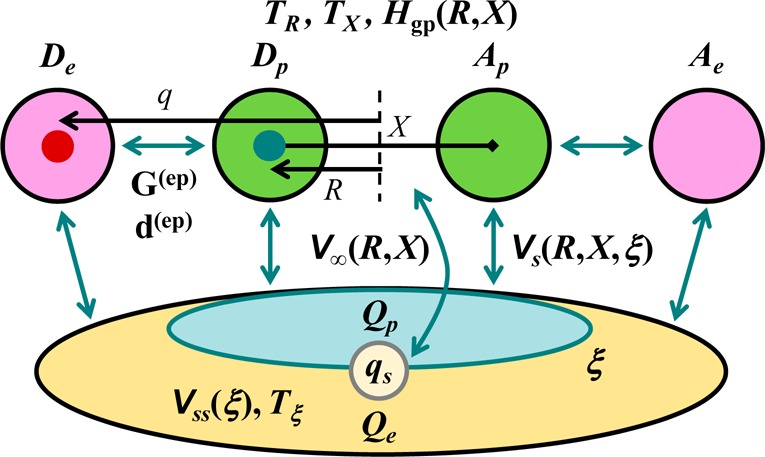
Schematic representation of the system and its interactions in the SHS theory of PCET. D_e (D_p) and A_e (A_p) are the electron (proton) donor and acceptor, respectively. Q_e and Q_p are the solvent collective coordinates associated with ET and PT, respectively. ξ denotes the overall set of solvent degrees of freedom. The energy terms in eqs 12.7 and 12.8 and the nonadiabatic coupling matrices d^(ep) and G^(ep) of eq 12.21 are depicted. The interactions between solute and solvent components are denoted using double-headed arrows.

Note that the time scale separation between the q_s (solvent electrons) and q (reactive electron) motions implies that the solvent “electronic polarization field is always in equilibrium with point-like solute electrons”.²¹⁴ In other words, the wave function for the solvent electrons has a parametric dependence on the q coordinate, as established by the BO separation of q_s and q. In addition, by using a strict BO adiabatic approximation¹¹⁴ (see section 5.1) for q_s with respect to the nuclear coordinates, the q_s wave function is independent of P_in(r). Ultimately, this implies the independence of V_∞ on Q_p and Q_e and the fact that the contributions to the free energy from the matrix elements in eq 12.9 do not depend on the continuum or molecular representation of the solvent and related effective Hamiltonian used (see below) to compute the free energy.

The free energy of the system for each VB state (i.e., the diabatic free energies) may be written as a functional of the solvent inertial polarization:^214,336,427

12.10

where is the self-energy of P_in(r) and includes the solute–solvent interaction and the energy of the gas-phase solute. G_n defines a PFES for the nuclear motion. G_n can also be written in terms of Q_p and Q_e.^214,428 Given the solute electronic state |ϕ_n⟩, G_n is^214,337

12.11

where, in a solvent continuum model, the VB matrix yielding the free energy is

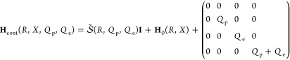12.12

and the adiabatic free energy surfaces are obtained by diagonalizing H_cont. In eq 12.12, I is the identity matrix. The function is the self-energy of the solvent inertial polarization field as a function of the solvent reaction coordinates expressed in eqs 12.3a and 12.3b. The initial solute–inertial polarization interaction (free) energy is contained in . In fact, the coordinate transformation inherent in the definitions of Q_p and Q_e shifts the zero of the solute–P_in interaction free energy to its initial value, and thus the ρ_Ia,Ia–P_in interaction energy is contained in the transformed term rather than in the last term of eq 12.12 that describes the solute–P_in interaction. Equation 12.11 represents a PFES (required for studying a charge transfer problem^429,430), and not just a PES, because the free energy appears in the averaging procedure inherent in the reduction of the many solvent degrees of freedom to the polarization field P_in(r).^193,429H_cont is a “Hamiltonian” in the sense of the solution reaction path Hamiltonian (SRPH) introduced by Lee and Hynes, which has the properties of a Hamiltonian when the solvent dynamics is treated at a nondissipative level.^429,430 Moreover, both the VB matrix in eq 12.12 and the SRPH follow closely in spirit the solution Hamiltonian central to the empirical valence bond approach of Warshel and co-workers,^431,432 which is obtained as a sum of a gas-phase solute empirical Hamiltonian and a diagonal matrix whose elements are solution free energies. For the VB matrix in eq 12.12, H_cont behaves as a VB electronic Hamiltonian that provides the effective PESs for proton motion.^191,337,433 This results from the equivalence of free energy and potential energy differences along R, with the assumption that the R dependence of the density differences in eqs 12.3a and 12.3b is weak, which allows the R dependence of to be disregarded just as it is disregarded for Q_p and Q_e.⁴³³ In addition, is approximately quadratic in Q_p and Q_e,^214,433 which leads to free energy paraboloids as shown in Figure 22c. The analytical expression for is^214,336

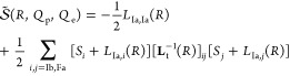12.13

where (S_Ia,S_Fa) ≡ (Q_p,Q_e), L is the reorganization energy matrix (a free energy matrix whose elements arise from the inertial reorganization of the solvent), and L_t is the truncated reorganization energy matrix that is obtained by eliminating the rows and columns corresponding to the states Ia and Fb. Equations 12.12 and 12.13 show that the input quantities required by the theory are electronic structure quantities needed to compute the elements of the VB Hamiltonian matrix for the gas-phase solute and reorganization energy matrix elements. Two contributions to the reorganization energy need to be computed: the inertial reorganization energy involved in and the electronic reorganization energy that enters H₀ through V_∞.

The inner-sphere (solute) contribution to the reorganization energy is not included in eq 12.12, but also needs to be computed when solute nuclear coordinates other than R change significantly during the reaction. The solute can even provide the predominant contribution to the reorganization energy when the reactive species are embedded in a molecular or solid matrix (as is often the case in charge transfer through organic molecular crystals^434−436), while the outer-sphere (solvent) reorganization energy usually dominates in solution (e.g., the X degree of freedom is associated with a small reorganization energy in the case of HAT, and this contribution can be disregarded compared to contributions from the solvent).

The inner-sphere reorganization energy λ_ij⁰ for charge transfer between two VB states i and j can be computed as follows: (i) the geometry of the gas-phase solute is optimized for both charge states; (ii) λ_ij for the i → j reaction is given by the difference between the energies of the charge state j in the two optimized geometries.^214,435 This procedure neglects the effects of the surrounding solvent on the optimized geometries. Indeed, as noted in ref (214), the evaluation of λ_ij⁰ can be performed in the framework of the multistate continuum theory after introduction of one or more solute coordinates (such as X) and parametrization of the gas-phase Hamiltonian as a function of these coordinates.

In a molecular solvent description, the reactive coordinates Q_p and Q_e are functions of solvent coordinates, rather than functionals of a polarization field. Similarly to eq 12.3a (12.3b), Q_p (Q_e) is defined as the change in solute–solvent interaction free energy in the PT (ET) reaction. This interaction is given in terms of the potential term V_s in eq 12.8, so that the solvent reaction coordinates are⁴³³

12.14a

12.14b

Both electrostatic and short-range solute–solvent interactions are included. The matrix that gives the free energy in the VB diabatic representation is

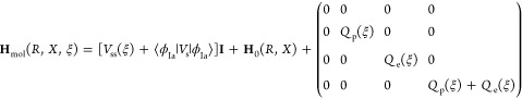12.15

The self-energy of the solvent is computed from the solvent–solvent interaction term V_ss in eq 12.8 plus the reference value (the zero) of the solvent–solute interaction in the coordinate transformation that defines Q_p and Q_e.

Equation 12.11 (or the analogue with H_mol) gives the free energy for each electronic state as a function of the proton coordinate, the intramolecular coordinate describing the proton donor–acceptor distance, and the two solvent coordinates. The combination of the free energy expression in eq 12.11 with a quantum mechanical description of the reactive proton allows computation of the mixed electron/proton states involved in the PCET reaction mechanism as functions of the solvent coordinates. One thus obtains a manifold of electron–proton vibrational states for each electronic state, and the PCET rate constant includes all charge-transfer channels that arise from such manifolds, as discussed in the next subsection.

12.2. Electron–Proton States, Rate Constants, and Dynamical Effects

After definition of the coordinates and the Hamiltonian or free energy matrix for the charge transfer system, the description of the system dynamics requires definition of the electron–proton states involved in the charge transitions. The SHS treatment points out that the double-adiabatic approximation (see sections 5 and 9) is not always valid for coupled ET and PT reactions.²²⁷ The BO adiabatic separation of the active electron and proton degrees of freedom from the other coordinates (following separation of the solvent electrons) is valid sufficiently far from avoided crossings of the electron–proton PFES, while appreciable nonadiabatic behavior may occur in the transition-state regions, depending on the magnitude of the splitting between the adiabatic electron–proton free energy surfaces. Applying the BO separation of the electron and proton degrees of freedom from the other (intramolecular and solvent) coordinates, adiabatic electron–proton states are obtained as eigenstates of the time-independent Schrödinger equation

12.16

where the Hamiltonian of the electron–proton subsystem, H_ep, is derived from eqs 12.7 and 12.8:

12.17

The eigenfunctions of H_ep can be expanded in basis functions, ψ_i, obtained by application of the double-adiabatic approximation with respect to the transferring electron and proton:²²⁷

12.18

Each ψ_j, where j denotes a set of quantum numbers {l,n}, is the product of an adiabatic or diabatic electronic wave function that is obtained using the standard BO adiabatic approximation for the reactive electron with respect to the other particles (including the proton)

12.19

and one of the proton vibrational wave functions corresponding to this electronic state, which are obtained (in the effective potential energy given by the energy eigenvalue of the electronic state as a function of the proton coordinate) by applying a second BO separation with respect to the other degrees of freedom:

12.20

The expansion in eq 12.18 allows an efficient computation of the adiabatic states Φ_i and a clear physical representation of the PCET reaction system. In fact, Φ_i has a dominant contribution from the double-adiabatic wave function (which we call ψ_i) that approximately characterizes the pertinent charge state of the system and smaller contributions from the other double-adiabatic wave functions that play an important role in the system dynamics near avoided crossings, where substantial departure from the double-adiabatic approximation occurs and it becomes necessary to distinguish Φ_i from ψ_i. By applying the same kind of procedure that leads from eq 5.10 to eq 5.30, it is seen that the double-adiabatic states are coupled by the Hamiltonian matrix elements

12.21

where d_ll′^(ep) and G_ll′ are defined as in eqs 5.18 and 5.31, respectively, but the derivatives are performed with respect to R only, and without using mass-weighted coordinates. m_p is the proton mass. The R subscript outside the brackets indicates integration over the proton coordinate R. These matrix elements are not neglected in the construction of the mixed electron–proton vibrational adiabatic states Φ_i, which are obtained as in eq 12.18 by solving the eigenvalue equation

12.22

where c is the matrix of the coefficients appearing in the expansion of eq 12.18 and E is the diagonal matrix with elements E_i. Ultimately, the procedure for obtaining the electron–proton states consists of (i) calculating the double-adiabatic states, and hence their matrix elements in eq 12.21, and (ii) replacing these matrix elements in eq 12.22, which is solved to obtain the expansion coefficients of Φ_i in eq 12.18. It is useful to construct ψ_j with an adiabatic electronic wave function if the ET reaction is near the adiabatic regime, while it is preferable to use a diabatic electronic wave function if the ET is in the nonadiabatic regime. The diabatic states may be given directly by the VB model. Moreover, the nonadiabatic states are related to the adiabatic states by a linear transformation, and eq 5.63 can be used in the nonadiabatic limit.

In deriving the double-adiabatic states, the free energy matrix in eq 12.12 or 12.15 is used rather than a standard Hamiltonian matrix.²¹⁴ In cases of electronically adiabatic PT (as in HAT, or in PCET for sufficiently strong hydrogen bonding between the proton donor and acceptor), the double-adiabatic states can be directly used since d_ll′^(ep) and G_ll′ are negligible.

In the SHS formulation, particular attention is paid to the common case of nonadiabatic ET and electronically adiabatic PT. In fact, this case is relevant to many biochemical systems^191,194 and is, in fact, well represented in Table 1. In this regime, the electronic couplings between PT states (namely, between the state pairs Ia, Ib and Fa, Fb that are connected by proton transitions) are larger than k_BT, while the electronic couplings between ET states (Ia–Fa and Ib–Fb) and those between EPT states (Ia–Fb and Ib–Fa) are smaller than k_BT. It is therefore possible to adopt an ET-diabatic representation constructed from just one initial localized electronic state and one final state, as in Figure 27c. Neglecting the electronic couplings between PT states amounts to considering the 2 × 2 blocks corresponding to the Ia, Ib and Fa, Fb states in the matrix of eq 12.12 or 12.15, whose diagonalization produces the electronic states represented as red curves in Figure 27b. Due to the electronically adiabatic behavior of the PT process, the excited state resulting from each 2 × 2 block diagonalization (upper red curves in Figure 27b) may be disregarded, so that only the two ground states of the 2 × 2 block diagonalizations remain (lower red curves in Figure 27b, reported in Figure 27c). Thus, the reactant and product states correspond to distinct ET diabatic states. The pertinent wave functions can be expanded on the basis of wave functions describing the VB states:

12.23a

12.23b

Each diabatic electronic state mixes PT states. Hence, the expansion coefficients depend on the solvent coordinate associated with the PT process. The dependence of the VB wave functions on nuclear coordinates is omitted, which is exact for strictly diabatic states. For the moment, the dependence on X is not considered explicitly. The energies corresponding to these diabatic states are¹⁹¹

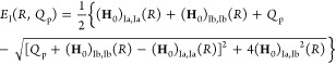12.24a

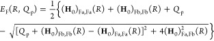12.24b

(where Q_p results from the semisum of the initial and final solute–P_in interaction energies and the subtraction of the initial one). Only the H_gp matrix elements (see eq 12.9) contribute to the coupling between the two electronic states. The electronic coupling averages over the reactant and product proton vibrational states, and it is given by

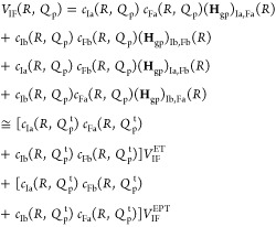12.25

where H_gp is the matrix that represents the solute gas-phase electronic Hamiltonian in the VB basis set. The second approximate expression uses the Condon approximation with respect to the solvent collective coordinate Q_p, as it is evaluated at the transition-state coordinate Q_p^t. Moreover, in this expression the couplings between the VB diabatic states are assumed to be constant, which amounts to a stronger application of the Condon approximation, giving

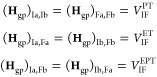12.26

These approximations are useful in applications of the theory, where V_IF^ET is assumed to be the same for pure ET and for the ET component of PCET reaction mechanisms and V_IF is approximated to be zero,¹⁹⁶ since it appears as a second-order coupling within the VB theory framework of ref (437) and is thus expected to be significantly smaller than V_IF^ET. The matrix corresponding to the free energy in the {ϕ_I,ϕ_F} basis is¹⁹¹

12.27

Under physically reasonable conditions for the solute–solvent interactions,^191,433 changes in the free energy H_JJ(R,Q_p,Q_e) (J = I or F) are approximately equivalent to changes in the potential energy along the R coordinate. The proton vibrational states that correspond to the initial and final electronic states can thus be obtained by solving the one-dimensional Schrödinger equation

12.28

The resulting electron–proton states are

12.29a

and

12.29b

where k (n) runs over the manifold of initial (final) proton vibrational states and the sets of quantum numbers μ = {I,k} and ν = {F,n} were introduced. The vibronic coupling is

12.30

In ref (196), the electronic coupling is approximated as in the second expression of eq 12.25 and the Condon approximation is also applied to the proton coordinate. In fact, the electronic coupling is computed at the value R = 0 of the proton coordinate that corresponds to maximum overlap between the reactant and product proton wave functions in the iron biimidazoline complexes studied. Thus, the vibronic coupling is written as

12.31

This vibronic coupling is used to compute the PCET rate in the electronically nonadiabatic limit of ET. The transition rate is derived by Soudackov and Hammes-Schiffer¹⁹¹ using Fermi’s golden rule, with the following approximations: (i) The electron–proton free energy surfaces ε_I^k(Q_p,Q_e) and ε_F(Q_p,Q_e) corresponding to the initial and final ET states are elliptic paraboloids, with identical curvatures, and this holds for each pair of proton vibrational states that is involved in the reaction. (ii) V_μν is assumed constant for each pair of states.

These approximations were shown to be valid for a wide range of PCET systems,⁴²⁰ and in the high-temperature limit for a Debye solvent¹⁴⁹ and in the absence of relevant intramolecular solute modes, they lead to the PCET rate constant

12.32

where P_μ is the Boltzmann distribution for the reactant states. In eq 12.32, the reaction free energy is

12.33

where (Q_p^μ,Q_e) and (Q_p^ν,Q_e) are the equilibrium solvent collective coordinates for states μ and ν, respectively. The outer-sphere reorganization energy associated with the μ → ν transition is

12.34

An inner-sphere contribution to the reorganization energy generally needs to be included.¹⁹⁶ The vibronic coupling W_μν(Q_p) from eq 12.30 is evaluated at the transition-state coordinate Q_p^t that corresponds to the intersection point of the μ and ν paraboloids along the straight-line reaction path connecting the minima of the PFESs (see Figure 22c). Thus, eq 12.31 is indeed used. As discussed in sections 5 and 10, the dependence of W_μν on the chemical structure and conformation of the system is dominated by the short-range exponential decrease of S_μν with the proton donor–acceptor distance, X, which is fixed in the derivation of eq 12.32. The theoretical accuracy of eq 12.32 makes its comparison with experimental data somewhat unfavorable, but it is particularly powerful where it is applicable (see ref (196), where excited proton vibrational states are included in the analysis).

Equation 12.32 has the multi-charge transfer channel form of eq 10.16. It differs from eq 11.6 in the attribution of a specific reorganization energy to each pair of proton vibrational states involved in the reaction, which reflects the possibility that the PFES minima are located at different positions for pairs of diabatic states μ and ν. The attribution of a specific reorganization free energy to each charge transfer channel arises naturally within the SHS theoretical framework. De facto, the major advance of eq 12.32, compared to previous expressions for this rate constant, is in the evaluation of the underpinning quantities. For example, the approximation that all proton vibrational states in one of the differently localized {χ_I^k} and {χ_F} manifolds interact in the same way with the solvent¹⁸⁸ is dropped in the SHS treatment. Cukier notes that the SHS analysis of PCET “has gone beyond this assumption and constructed a continuum-based theory that accounts for specific effects of solvation on the various proton states that are coupled in the transfer”.¹⁹⁰ Moreover, all of the involved quantities (vibronic couplings, reaction free energies, and reorganization energies) are computed for consistently derived two-dimensional mixed electron–proton vibrational free energy surfaces. Within this framework, it is shown that λ_μν is not simply the sum of the reorganization energies for pure PT and ET, because of a term that arises from the interaction of the change in density caused by one charge transfer process with the variation of the inertial polarization field resulting from the change in density produced by the other charge transfer process. All such features also distinguish eq 12.32 from similar rate constants previously obtained for pure ET involving nuclear modes that are treated quantum mechanically.^340,342,343 Furthermore, the coupling of the transferring proton with the solvent, which is critical in PCET, does not allow use of the rate expression with the quantities computed for the ET problem just by identifying the proton as an inner-sphere solute mode, although the formalism developed to tackle the intramolecular modes in ET systems^340,342,343 can be exploited to formulate PCET rate constants.¹⁹¹

Effects of the intramolecular mode X are introduced in the SHS treatment in two different ways, depending on the value of the X vibrational frequency. When the X mode is characterized by a slow frequency and is not coupled dynamically to the solvent fluctuations, a parametric dependence of the electron–proton free energy surfaces, ε_I^k(X,Q_p,Q_e) and ε_I(X,Q_p,Q_e), on X is included in the SHS analysis. A rate constant for the reactive system equilibrated at each X value can be written as in eq 12.32, and the overall observed rate is

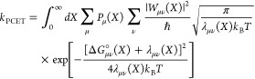12.35

The opposite limit of a very fast X mode requires that X be treated quantum mechanically, similarly to the reactive electron and proton. Also in this limit X is dynamically uncoupled from the solvent fluctuations, because the X vibrational frequency (ω) is above the solvent frequency range involved in the PCET reaction (in other words, ω is out of the solvent frequency range on the opposite side compared to the case leading to eq 12.35). This limit can be treated by constructing electron–proton–X mode states, with the same procedure used to obtain electron–proton states in eqs 12.16–12.22 but in the presence of two nuclear modes (R and X). The rate constant for nonadiabatic PCET in the high-temperature limit of a Debye solvent has the form of eq 12.32, except that the involved quantities are calculated for pairs of mixed electron–proton–X mode vibronic free energy surfaces, again assumed harmonic in Q_p and Q_e.

The most common situation is intermediate between the two limiting cases described above. X fluctuations modulate the proton tunneling distance, and thus the coupling between the reactant and product vibronic states. The fluctuations in the vibronic matrix element are also dynamically coupled to the fluctuations of the solvent that are responsible for driving the system to the transition regions of the free energy surfaces. The effects on the PCET rate of the dynamical coupling between the X mode and the solvent coordinates are addressed by a dynamical treatment of the X mode at the same level as the solvent modes. The formalism of Borgis and Hynes is applied,^165,192,193 but the relevant quantities are formulated and computed in a manner that is suitable for the general context of coupled ET and PT reactions. In particular, the possible occurrence of nonadiabatic ET between the PFES for nuclear motion is accounted for. Formally, the rate constants in different physical regimes can be written as in section 10. More specifically:

(i) In the high-temperature and/or low-frequency regime for the X mode, ℏω/k_BT ≪ 1, the rate is^337,345

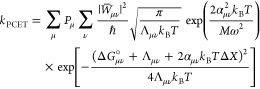12.36

The formal rate expression in eq 12.36 is obtained by insertion of eq 10.17 into the general term of the sum in eq 10.16. If the reorganization energy is dominated by the solvent contribution and the equilibrium X value is the same in the reactant and product vibronic states, so that ΔX = 0, eq 12.35 simplifies to¹⁸⁴

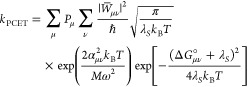12.37

In the low temperature and/or high frequency regime of the X mode, as defined by ℏω/k_BT ≫ 1, and in the strong solvation limit where λ_S > |ΔG°|, the rate is

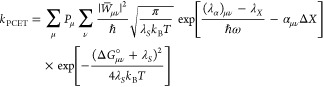12.38

as is obtained by insertion of eqs 10.18 into eq 10.16. Useful analysis and application of the above rate constant expressions to idealized and real PCET systems is found in studies of Hammes-Schiffer and co-workers.^{184,225,337,345,421}

12.3. Note on the Kinetic Isotope Effect in PCET

Hammes-Schiffer and co-workers have emphasized that KIE is a hallmark of concerted PCET reaction mechanisms.¹⁸⁴ When the concerted ET–PT reaction is electronically nonadiabatic (in contrast to the typically electronically adiabatic HAT), the PCET rate constant depends on squared vibronic couplings, which can be approximated as products of (squared) electronic couplings and overlaps between the reactant and product proton vibrational functions. For simplicity, we restrict the discussion here to a pair of vibrational states, for example with the assumption that only the ground diabatic proton states are involved in the reaction. According to the rate expressions for electronically nonadiabatic PCET given in section 12.2, the ratio of the PCET rate constants for hydrogen (or, in more rigorous terms, protium), H, and deuterium, D, will depend on the ratio |S_H|²/|S_D|², which is significantly larger than unity due to the difference in the H and D masses and to the exponential dependence of the wave function overlap on the mass of the tunneling particle (see eq 7.11). Equation 7.11, written for arbitrary donor–acceptor distances, also shows that the difference in mass causes a sharper distance dependence for S_D than for S_H, so α_D > α_H. For systems that are in relatively rigid reactive conformations (for example, in enzyme active sites with short hydrogen donor–acceptor distances, less than the sum of van der Waals radii, which is in the 3.2–3.5 Å range²⁹⁷), the terms arising from X coordinate thermal fluctuation (see eqs 12.36–12.38) can be disregarded and the KIE is determined by |S_H|²/|S_D|². Thus, in these systems the KIE essentially does not depend on the temperature. In the range of validity of eq 12.37, with the further simplifying assumption that reaction free energy and reorganization energy isotope effects such as in eq 6.27 are not significant, one finds

12.39

which implies that KIE decreases with increasing temperature. In this regime, KIE depends on |S̅_H|²/|S̅_D|², on the frequency ω of the X mode, and on the X dependence of the vibrational (and hence vibronic) coupling. Thus, a key role is played by the X mode characteristics.⁴³⁸ The interpretation of KIEs can be very complicated, even under the above simplifying assumptions, if excited vibrational states are involved in the reaction mechanism. Moreover, both contributions to KIE in eqs 6.27 and 12.39 generally need to be considered, as is done in ref (438).

12.4. Distinguishing between HAT and Concerted PCET Reactions

The SHS framework provides a fruitful scheme to distinguish among different reaction mechanisms involving both ET and PT. Of particular interest is the distinction between the HAT and concerted PCET reaction mechanisms. As noted by Cukier, “Deciding whether electron and proton transfer is a consecutive or a concerted process can be quite difficult, from both experimental and theoretical perspectives. Distinguishing between PCET and HAT also can be difficult.” ¹⁹⁰

A clear difference between HAT and EPT is that HAT involves the same electron and proton donor and acceptor, while the EPT is characterized by ET and PT between two different redox pairs. However, strictly speaking, “This criterion is not rigorous because the electron and proton behave quantum mechanically and hence are not localized to a specific point at any given time.” ²¹⁵ A consistent quantum mechanical treatment of the electron and proton degrees of freedom would address this issue, and, at any rate, the mentioned argument affords in all contexts the major criterion for the differentiation between the two reactions.

Distinctive features of HAT are the very small value of the associated solvent reorganization energy due to the correspondingly weak influence of the neutral transferring particle on the surrounding charge distribution (e.g., in ref (196) a relatively large outer-sphere reorganization energy indicates that concerted PCET and not HAT is the mechanism for iron biimidazoline complexes) and the electronic adiabaticity of the reaction that arises from the short ET path for the electron bound to the proton, at odds with the electronically nonadiabatic character of several PCET reactions in biological systems. Both HAT and EPT are usually vibronically nonadiabatic, due to the small proton wave function overlap that produces vibronic couplings much less than k_BT.¹⁹⁷ In fact, vibronic nonadiabaticiy is the most frequent case in Table 1 (see the last two columns), where PT is electronically adiabatic but vibrationally nonadiabatic.

A quantitative discriminator for HAT versus EPT is the degree of electronic nonadiabaticity for the PT process.^195,197 The parameter p (eq 7.4) formulated for EPT reactions¹⁹⁵ was applied by Hammes-Schiffer and co-workers to distinguish between HAT and EPT. When, in eq 7.10, the time for proton tunneling is much longer than the time for the electron transition, the proton sees the mix of the initial and final diabatic electronic states; namely, the PT occurs on the electronically adiabatic ground state as expected for HAT. In the case in which p = τ_p/τ_e ≪ 1, an electronically nonadiabatic reaction is operative, as is expected for concerted electron–proton transfer with a D_e–A_e distance much larger than the D_p–A_p distance. PCET reactions can also be in the intermediate regime, thus complicating discrimination of the reaction mechanisms.

The above diagnostic criterion was applied to the phenoxyl/phenol and benzyl/toluene systems (Figure 48) at their transition-state geometries. A strong hydrogen bond approximately planar with the phenol rings is observed in the first case, while a weaker hydrogen bond nearly orthogonal to the benzene rings is obtained in the second case. The singly occupied Kohn–Sham molecular orbitals³² are dominated by 2p orbitals perpendicular to the D_p–A_p axis for the phenoxyl/phenol system, while they are dominated by σ orbitals oriented along the D_p–A_p axis in the benzyl/toluene system. In ref (32), this molecular orbital arrangement led to the conclusion that EPT takes place in the first case, while HAT occurs in the second case, where the two charges transfer between the same donor and acceptor groups. This conclusion is confirmed and quantified by application of the adiabaticity degree parameter p in ref (197), since p = 1/80 for phenoxyl/phenol and 4 for the benzyl/toluene system (see also the potential energy curves in Figures 22a,b).

Figure 48.

The two highest occupied electronic Kohn–Sham orbitals for the (a) phenoxyl/phenol and (b) benzyl/toluene systems. The orbital of lower energy is doubly occupied, while the other is singly occupied. I is the initial diabatic state (charges on the donors), II is the final one (F in the notation of this review), and TS denotes the transition state. Reprinted from ref (197). Copyright 2006 American Chemical Society.

12.5. Electrochemical PCET

The analysis by Hammes-Schiffer and co-workers has also been extended to electrochemical PCET, combining the nonadiabatic PCET rate expression with methods previously developed for the study of electrochemical ET.³⁵⁷ Figure 49 shows a typical electrochemical PCET system to which the proposed theoretical setup can be applied. It is composed of a metal electrode, M, in contact with a solution containing electrolyte ions and solute molecules (the solute complex in Figure 49) that can exchange electrons with the electrode and can carry out a PT along a hydrogen bond inside the complex. In modeling the system, the ET reaction occurs only after formation of the solute complex (SC) with the hydrogen bond scenario of the PT reaction. The PCET mechanism is characterized by nonadiabatic transitions between reactant and product vibronic states. An important environmental coordinate to be included in the analysis is the electrode–SC distance x. A special value of x is the distance x_H of the outer Helmholtz plane (OHP in Figure 49) from M, which is the distance of closest approach to the electrode for the solvated solute complex. Another relevant coordinate is the proton donor–acceptor distance X (denoted by R in Figure 49, as reproduced from ref (357), while R is reserved for the proton coordinate in our review). M is described as a free-electron reservoir with (unbiased) Fermi level ε_M. The electrical double layer determined by the equilibrium distribution of the electrolyte ions near the electrode–solution interface leads to the electrostatic potential field ϕ_s(x) in the absence of SC, and the zero of this potential is taken in the bulk solution, at practically infinite distance from the metal: ϕ_s(x→∞) = 0. Beyond the OHP, in the diffuse layer, ϕ_s(x) decreases exponentially with the distance from the interface as described by the Gouy–Chapman-Stern model of the double layer.^439−441

Figure 49.

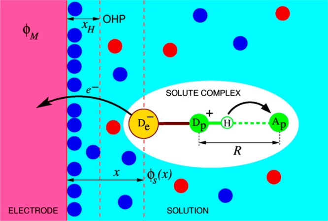
Schematic representation of the electrochemical PCET model system of Hammes-Schiffer and co-workers. The filled circles represent the electrolyte ions in the solution. ϕ_M denotes the inner potential of the electrode, while ϕ_s(x) is the electrostatic potential in solution at a distance x from the metal surface. x_H locates the OHP. R denotes the proton donor–acceptor distance, which is denoted X throughout this review. Reprinted with permission from ref (357). Copyright 2008 American Chemical Society.

The transfer rate or transition probability per unit time from the reduced SC to the M level of energy ε at a given M–SC distance x can be written using one of the expressions in section 12.2, depending on the temperature and the frequency of the intramolecular mode X. In the electrochemical setup, the expression for the driving force ΔG_μν°, now written as ΔG_μν(η,x,ε), reflects the presence of a heterogeneous interface, involving a metal, and depends on the applied overpotential η:

12.40

In eq 12.40, ΔU_μν is the difference between the minima of the free energy surfaces for the oxidized and reduced SC in bulk solution, i.e., in the absence of the electrode. Q_I and Q_F are the partition functions of the reduced (initial) and oxidized (final) SC, respectively, in bulk solution.

Hammes-Schiffer and co-workers assumed that eq 12.36, with the free energy of reaction given by eq 12.40, is the most relevant expression for the oxidation rate . ΔX has a different sign for the cathodic and anodic currents. Consequently, the 2α_μvk_BTΔX term in the effective activation energy has opposite signs in the reduction rate and in the oxidation rate (which causes asymmetry of the theoretical Tafel plot), and according to eq 10.4, the respective vibronic couplings, hence the overall rates, differ by the factor exp(−2α_IFΔX). Introducing the metal density of states ρ(ε) and the Fermi–Dirac occupation distribution f(ε) = [1 + exp(ε/k_BT)]⁻¹, with energies referred to the Fermi level, the oxidation and reduction rates are written in the Gurney⁴⁴²–Marcus^122,234–Chidsey⁴⁴³ form:

12.41a

12.41b

The anodic, j_a, and cathodic, j_c, current densities (corresponding to the SC oxidation and reduction processes, respectively) are related to the rate constants in eqs 12.41a and 12.41b by^357,444

12.42a

12.42b

where denotes the Faraday constant and C_SC(η,x) and C_SC⁺(η,x) are the molar concentrations of the reduced and oxidized SC, respectively. Evaluation of eqs 12.42a and 12.42b has been performed under several simplifying assumptions. First, it is assumed that, in the nonadiabatic regime resulting from the relatively large value of x_H and for sufficiently low total concentration of the solute complex, the low currents in the overpotential range explored do not appreciably alter the equilibrium Boltzmann distribution of the two SC redox species in the diffuse layer just outside the OHP and beyond it. As a consequence,

12.43

where CSC+0(η,x) and CSC(η,x) are bulk concentrations. The vibronic coupling is approximated as VIFETSμv, with Sμvp satisfying eq 9.21 for (0,n) → (μ,ν) and VIF decreasing exponentially with x as exp(−βETx/2). The Debye length characterizing the thickness of the diffuse layer357 (or, as a simple alternative, xH) is assumed to be much larger than βET–1, and thus in the allowed x range the current is dominated by the contribution at xH. Additional approximations are that the double layer effect can be neglected, the density of states of the electrode can be approximated with its value ρF at the Fermi level, VIFET is independent of the metal electronic level, and the initial and final proton states are well described by harmonic oscillators with equal frequency ωp. The total current density is then expressed in the form215,357

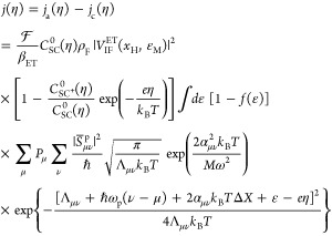12.44

The overpotential is referenced to the formal potential of the redox SC. Therefore, CSC+0(η,x) = CSC(η,x) and j(η) = 0 for η = 0.

Reference (357) emphasizes that replacing the Fermi function in eq 12.44 with the Heaviside step function, to enable analytical evaluation of the integral, would lead to inconsistencies and violation of detailed balance, so the integral form of the total current is maintained throughout the treatment. Indeed, the Marcus–Hush–Chidsey integral involved in eq 12.44 has imposed limitations on the analytical elaborations in theoretical electrochemistry over many years. Analytical solutions of the Marcus–Hush–Chidsey integral appeared in more recent literature^445,446 in the form of series expansions, and they satisfy detailed balance. These solutions can be applied to each term in the sums of eq 12.44, thus leading to an analytical expression of j without cumbersome integral evaluation. Moreover, the rapid convergence⁴⁴⁷ of the series expansion afforded in ref (446) allows for its efficient use even when several vibronic states are relevant to the PCET mechanism. Another rapidly convergent solution of the Marcus–Hush–Chidsey integral is available from a later study⁴⁴⁸ that elaborates on the results of ref (445) and applies a piecewise polynomial approximation.

Finally, we mention that Hammes-Schiffer and co-workers⁴⁴⁹ have also examined the definition of a model system-bath Hamiltonian for electrochemical PCET that facilitates extensions of the theory.

A comprehensive survey of theoretical and experimental approaches to electrochemical PCET was provided in a recent review.⁴⁵⁰

13. Conclusions and Prospects

Increasingly powerful interpretative and predictive models for independent and coupled electron, proton, and atom transfer have emerged in the past two decades. An “ideal” theory is expected to have the following characteristics:

(i) Quantum description of the transferring proton(s) and other relevant degrees of freedom, such as the proton donor–acceptor distance.

(ii) Relaxation of the adiabatic approximation inherent in the BO separation of electronic and nuclear motion. In several cases the nonadiabatic coupling terms neglected in eq 5.8 are precisely those terms that are responsible for the transitions between states with different electron charge localizations.

(iii) Capacity to describe the transferring electron(s) and proton(s) in a similar fashion and to capture situations ranging from the adiabatic to the nonadiabatic regime with respect to other degrees of freedom.

(iv) Consideration of the adiabatic, nonadiabatic, and intermediate regimes arising from the relative time scales of the dynamics of active electron(s), transferring proton(s), and other relevant nuclear modes.

(v) Ability to classify and characterize diverse PCET reactions, establishing analogies and differences that enable predictions for novel systems and also suggestions for de novo designs of artificial systems. The relationship between partition in subsystems and adiabatic/nonadiabatic behaviors, on the one hand, and structure/function features, on the other hand, needs to be suitably addressed.

(vi) Theoretical analysis of the structural fluctuations involved in PCET reactions leading a system to access different mechanistic regimes.

(vii) Theoretical connection of various PCET regimes and pertinent rates, and the related identification of signatures of transitions from one regime to the other, also in the presence of fluctuations of the relevant charge transfer media. A very recent study by Koper¹⁸⁵ proposes a theoretical model to compute potential energy surfaces for electrochemical PCET and to predict the transition form sequential to concerted electron–proton transfer induced by a changing overpotential. Regarding direct molecular dynamics simulation of PCET across multiple regimes, apart from the well-known surface-hopping method,^{119,160,167,451} an interesting recent study of Kretchmer and Miller¹⁸⁶ proposes an extension of the ring polymer molecular dynamics method^452,453 that enables the direct simulation of PCET reactions across a wide range of mechanistic regimes.

(viii) Identification of robust markers of single-charge transfer reactions that allow their tracking in complex mechanisms that involve coupled charge transfer processes.

(ix) Points v–viii may motivate strategies to induce adiabatic or nonadiabatic behaviors in PCET reactions. Addressing these many challenging points may require the development of new theories and computational techniques or a combination of existing strategies.

(x) Conceptual and analytical simplifications of the theory may remove unimportant or difficult to observe refinements that prevent comparison with experiments, in order to define parameters and signatures outlined in items v–ix. Interplay between theory and experiment seems essential for achieving all of these goals.

These 10 aims seem likely to drive developments in the field of PCET reaction mechanisms. Some of these requirements were stressed and addressed to some extent in the studies that were reviewed above. The analyses of Hammes-Schiffer, Soudackov, and co-workers (refs (160, 164, 167, 182, 184, 191, 194, 196, 214, 215, 225, 227, 337, 345, 357, 420, and 454−461)) comprehensively addressed issues i–iv and partially addressed issues v and vi. Points v and vi and vii–x remain largely open. A few recent studies^185,186 have been focused on issue vii. Theory that was applied widely to investigate fluctuations in biological ET^{316,318,462−472} may be extended fruitfully to account for items vi and vii. Furthermore, such an extension may provide support to satisfy aims vii–x. In particular, point x is a major issue encompassing almost all other issues. Some authors have recently noted that, “A few papers have applied versions of Hammes-Schiffer’s multistate continuum theory, although this is challenging, and simplifications usually have to be applied because many of the needed parameters are not easily accessible.” ²⁴⁸ For this reason, the extended semiclassical Marcus model, based on the Marcus–Hush–Levich formalism, has been preferred to interpret experimental data in several applications.^450,473 Importantly, the semiclassical Marcus model can be derived from the multistate continuum theory with the assumptions that the free energy depends on a single solvent coordinate and that the electronic states can be approximated using the two-state model in the weak-coupling limit.^214,336 Previous studies (e.g., see ref (184) and references therein) and our review provide connections among recent PCET theories and among these theories and the extended Marcus theory. However, future efforts in this direction are needed to elaborate analytical PCET rate expressions that are more inclusive than Marcus’ rate (in particular, with respect to proton tunneling and specific treatment of relevant nuclear coordinates) but less comprehensive than those provided by Hammes-Schiffer and co-workers. Such expressions may favor more direct explorations of experimental data within specific classes of PCET reactions.

Despite the significance of point x above, the importance of the multistate continuum theory and its developments for understanding the nature of PCET reaction mechanisms (even in sophisticated formulations that did not introduce substantial levels of approximation) was demonstrated by successful comparisons with experiments in the past decade.^{196,421,474−481} In addition, further development on the experimental side will continue to allow increasingly detailed and direct comparisons with theory. Further developments of the strategies of Cukier, Borgis and Hynes, and Hammes-Schiffer and co-workers addressing issues v–x would be useful as well. As discussed in ref (182), the ability to classify PCET reactions plays a critical role in understanding basic principles underlying a wide range of natural, engineered, and artificial systems for energy conversion and of interest in growing efforts to develop alternative renewable energy sources. In this respect, significant progress can be made by the systematic investigation of the limiting forms of equations and rate constants involving multiple vibronic states and understanding the limits of validity of the inherent simplifications. It is important to gain a deeper understanding of the essential features that make the extended Marcus theory successful for describing charge transfer reactions (beyond outer-sphere ET reactions), its limitations, and what generic features (such as eq 6.20 and the rightmost term in eq 6.25) can be fruitfully specified to extend its applicability further and to link the theory to recent PCET theories. A useful example of the connection between the extended Marcus theory and a more specific treatment of PT is provided by the way in which eq 6.12 is found again in the treatment of homogeneous PT by Levich et al.,¹⁸⁰ and other connections are described in our review. The Hopfield treatment of nuclear modes³⁰⁸ may serve as an “intermediary” between the Marcus and the Borgis–Hynes and SHS theories of PCET in regimes where its semiclassical description of the transition between classical and quantum nuclear motion is adequate.

A consistent description of quantum effects (including zero-point energy and nuclear tunneling) is provided by the wave packet dynamical method through use of ab initio molecular dynamics combined with the description of the tunneling particle as a quantum wave packet.^482−485 The evolving wave packet is thus coupled to changes in the surrounding electronic structure and nuclear geometry.

Even where simplifications to the formalism of the SHS theory are possible, the framework of system coordinates and states in the SHS treatment of PCET should be retained, because it yields a profitable approach to classify PCET reactions and to relate them to the experimental context. The combination of rich and predictive theories with experimental systems that are absolutely central to molecular bioenergetics and to solar fuel production are likely to make this direction of research of increasing significance and impact in the coming decades.

Glossary

Glossary

|0⟩

vacuum state with respect to the electronic active space

A, A_e, A_p

acceptor, electron acceptor, proton acceptor

AA

amino acid

a

classical turning point distance relative to a PES minimum for the H particle in BH theory

A₁, A₂ (or A, B)

molecular groups involved in hydrogen atom transfer

A_if^kn

PT rate constant prefactor in generalized Cukier theory, defined by eq 11.24b

ad (nonad)

adiabatic (nonadiabatic)

α_IF

decay factor for the proton wave function overlap or for the vibronic coupling

α, β

spin components or functions in section 12.1

α, β subscripts

used to distinguish adiabatic wave functions

BEBO

bond energy–bond order method

BLUF

blue light using flavin adenine dinucleotide

BH

Borgis–Hynes

BO

Born–Oppenheimer

Br

bridge

b (b_t)

degree-of-reaction parameter (at the transition state); see section 6.1

b_n

bond order in BEBO

bpy

2,2′-bipyridine

β

Brønsted, or Leffler, slope in section 6; (k_BT)⁻¹ in Appendix A

β_ET

decay factor of the squared electronic coupling

C

inefficient precursor complex in eq 8.2

C_X (C_S)

time autocorrelation function for the fluctuations of the X (S) nuclear mode

C_SC (C_SC^–)

molar concentration of the reduced (oxidized) SC (section 12.5)

c_e (c_p)

coupling of the reactive electron (proton) charge with the solvent polarization in the Cukier PES model for ET–PT

c_n

nth coefficient in the system wave function expansion

c_p

Pekar factor

γ

electron–proton coupling strength in Cukier theory

D, D_e, D_p

donor, electron donor, proton donor

D_J

electric displacement corresponding to the equilibrium inertial polarization in the J (= I or F) electronic state

D

deuterium

DKL

Dogonadze–Kuznetsov–Levich

Δ₁₂

diabatic energy difference in the model of Figure 24

ΔE°

potential energy difference replacing ΔG° in gas-phase reactions

ΔE^el

gas-phase electronic structure contribution to the reaction free energy

ΔE* (ΔG*)

activation (free) energy

ΔE_S

reaction free energy, or “asymmetry”, along the S coordinate (section 10)

ΔE_X

reaction free energy, or “asymmetry”, along the X coordinate (section 10)

ΔF

proton PES slope difference at R_t in the Georgievskii and Stuchebrukhov model

ΔG° (ΔG_R°)

reaction free energy (in the prevailing medium at mean D–A distance R)

ΔG^solv

solvation contribution to the reaction free energy

ΔH

splitting between the H levels in reactants and products (section 10)

ΔR_e

proton coordinate range where the electron transition can occur with appreciable probability in the Georgievskii and Stuchebrukhov model

ΔU_μν

difference between the PFES minima for the oxidized and reduced SC in bulk solution (section 12.5)

d

distance between the electron D and A centers in the Cukier ellipsoidal model

d^(ep) and G^(ep)

nonadiabatic coupling matrices defined via eq 12.21

d_kn

nonadiabatic coupling vector involving the k and n electronic functions

dmp

4,7-dimethyl-1,10-phenanthroline

δ_kn (δ)

Kronecker (Dirac) δ

δR_n

width parameter of the nth proton vibrational wave function χ_n^p

δX (δS)

fluctuation of the X (S) coordinate

ΔX (ΔS)

coordinate shift between the free energy minima along X (S)

E_a

activation energy (see section 9)

E_f

formation energy of the reactive complex in the Marcus model using BEBO

E_ik (E_fn)

energy eigenvalue associated with the vibrational function χ_k^X (χ_n)

E_n(R,Q)

electronic energy for the nth electronic (basis) state

E̅_n(R)

average of E_n(R,Q) over state |χ_n⟩

E̅_n^p(Q)

average of E_n(R,Q) over state |χ_n^p⟩

total energy

ET

electron transfer

EPT

electron–proton transfer (concerted PCET)

ET/PT (PT/ET)

coupled, sequential ET and PT, with ET preceding (following) PT

ET–PT

ET/PT, PT/ET, or EPT

e

absolute value of the electron charge

ε

dielectric constant

ε_a

intrinsic asymmetry parameter (section 6.1)

ε_s

static dielectric constant

ε_∞

optical dielectric constant

ε_Jμ or ε_Jμ^p

vibrational energy of the μth proton state in the J (= I or F) electronic state

ε_M

metal Fermi level

Faraday constant

f

dimensionless magnitude of the effective displacement of X (when X is in angstroms) (used in section 5.3)

f₁₂

dimensionless factor in Marcus cross-relation, defined by eq 6.6 or 6.10

f_α ^J

fraction of electron charge located at r_α in the J (= I or F) electronic state in Cukier’s treatment of the reorganization and solvation free energies

f_β ^J

fraction of proton charge located at r_β in the J (= I or F) electronic state in Cukier’s treatment of the reorganization and solvation free energies

f(ε)

Fermi–Dirac distribution (section 12.5)

G_kn

nuclear kinetic nonadiabatic coupling defined by eq 5.31

G_J^solv(R)

equilibrium solvation free energy contribution to the effective potential for proton motion in the J (= I or F) electronic state

G

free energy

g₁, g₂

real functions introduced in eq 6.19 and normalized so that g(1/2) = 1

g_j

coupling of the jth solvent mode with the tunneling electron in Cukier theory

ζ_GROUP

active-electron orbital on GROUP = D_e, A_e, D_p, or A_p transferring H species

H

tunneling particle that may be a proton or a hydrogen atom

or H_tot

Hamiltonian

H or H_el

electronic Hamiltonian

H₀

channel Hamiltonian in the model of Figure 24

H₀

Hamiltonian matrix including the gas-phase solute energy and solute–solvent electronic polarization interaction in the four-state VB basis of section 12

H_cont

VB matrix yielding the free energy in the SHS multistate continuum theory

H_mol

counterpart of H_cont with molecular description of the solvent

H_ep (H_ep)

Hamiltonian (matrix) for the reactive electron–proton subsystem

H^g

gas-phase solute Hamiltonian (see Cukier’s model in section 11)

H_gp

gas-phase solute electronic Hamiltonian (see SHS model in section 12.1)

H_p

Hamiltonian associated with the proton in Cukier’s theory

ℏ

reduced Planck constant

HAT

hydrogen atom transfer

H₂bim

2,2′-biimidazoline

HOH

water

η

overpotential

1 or I index

initial electronic state

2 or F index

final electronic state

i (f) index

initial (final) proton state (section 11)

j_a (j_c)

anodic (cathodic) current density

J_IF

flux correlation in BH expression of the current

K₁₂

equilibrium constant for Ox₁ + Red₂ ⇌ Red₁ + Ox₂

KSE

kinetic solvent effect

k_B

Boltzmann constant

k_d

diffusion constant

k_REACTION

rate constant for REACTION = ET, PT, HAT, and PCET

k_H (k_D)

protium (deuterium) transfer rate constant

|k_I⟩ (|n_F⟩)

proton vibrational state associated with the I (F) electronic state

κ

factor in the Georgievskii and Stuchebrukhov expression of the vibronic coupling, defined in eq 7.3

κ_el

electronic transmission coefficient

L

reorganization energy matrix in the SHS multistate continuum theory

LBHB

low-barrier H-bond

L_t

truncated reorganization energy matrix in the SHS multistate continuum theory

Λ

total reorganization energy in BH and SHS treatments including fluctuations of the charge-transfer nuclear medium

λ

reorganization energy

λ_α

coupling reorganization energy for i → j VB charge-state transition

λ_H (λ_D)

reorganization energy associated with hydrogen (deuterium) transfer

λ_ij⁰

inner-sphere reorganization energy for the i → j reaction

M

nuclear mass; more specifically, mass associated with the X nuclear mode in sections 9–12

M

metal electrode

MLCT

metal-to-ligand charge transfer

M_S

mass associated with the collective solvent mode S

MS-EPT

multiple-site electron–proton transfer

m

electronic mass

met

Fe(III)Fe(III) state of the diiron cofactor

m_H

mass of the tunneling proton or hydrogen atom in BH theory

m_p

proton mass

NHE

normal hydrogen electrode

ν

vibrational frequency

ν_n

effective nuclear frequency for the reaction coordinate motion

ν_el

ET frequency in the activated complex (eq 5.28b)

ξ

set of solvent degrees of freedom (section 12)

ξ_n

c_nχ_n

OHP

outer Helmholtz plane

p

proton adiabaticity parameter in the Georgievskii and Stuchebrukhov model

P

nuclear momentum

(P_in,J)P_J

(inertial or orientational) polarization in the J (= I or F) electronic state

PCET

proton-coupled electron transfer

PES

(effective) potential energy surface

PFES

(effective) potential free energy surface

P_μ

Boltzmann probability of the μth proton state in the reactant electronic state

p_n

power of b_n in the Marcus equations using BEBO

P(X)

thermally averaged X probability density (section 11)

PT

proton transfer

Q (q)

nuclear (electronic) coordinate

Q_e

collective solvent coordinate driving ET

Q_p

collective solvent coordinate driving PT

Q_pe

overall solvent reaction coordinate in EPT mechanisms

Q_t

transition state coordinate

±q₀

average electron position in its I (−) and F (+) equilibrium states (section 11)

q_i

coordinates of core electrons

q_S

coordinates of “infinitely” fast solvent electrons

R (R_t)

coordinate of the transferring proton (at the transition state)

±R₀

equilibrium proton position in the I (−) and F (+) electronic states (section 11)

R_A···B or R_AB

proton donor–acceptor distance

RC

reaction center

r

position vector

r

edge-to-edge distance between the electron donor and acceptor (section 8)

r_s

radius of the spheres that represent the electron donor and acceptor groups in the continuum ellipsoidal model adopted by Cukier

r_ij, r_αβ, r_iα

distances between electronic, nuclear, and electronic–nuclear positions

ρ

one-electron density

ρ_cl(X)

probability density of an X classical oscillator

ρ(ε)

metal density of states (section 12.5)

RNR

ribonucleotide reductase

S

collective solvent coordinate

self-energy of the solvent inertial polarization in multistate continuum theory

transformed , namely, as a function of the coordinates in eqs 12.3a and 12.3b

SC

solute complex (section 12.5)

SHS

Soudackov–Hammes-Schiffer

S_kn (S_kn^p)

overlap between the χ_k (χ_k^p) and χ_n (χ_k) vibrational wave functions

SRPH

solution reaction path Hamiltonian

σ̂_x, σ̂_z

Pauli matrices

T

temperature

t_1/2

half-life

_IF

transition probability density per unit time, eq 5.3

T_n (T_n^p)

nuclear kinetic energy in state |χ_n⟩ (|χ_n^p⟩)

T̂_Q, T̂_R, T̂_ξ, T̂_q

nuclear, reactive proton, solvent, and electronic kinetic energy operators

τ_el

lifetime of the initial (before ET) electronic state

τ_p

proton tunneling time

θ

rotation angle connecting two-state diabatic and adiabatic electronic sets

θ_p

dimensionless nuclear coupling parameter, defined in eq 9.8

u_if^kn

PT Landau–Zener parameter

V

potential energy

VB

valence bond

V_c

potential energy at PES crossing in the Georgievskii and Stuchebrukhov model

V_IF

(effective) electronic coupling

Ṽ_IF

effective electronic coupling between nonorthogonal diabatic electronic states

_in(r)

electrostatic potential field generated by the inertial polarization field

V_∞

interaction potential between solute and solvent electronic degrees of freedom

V_J^g(R)

gas-phase potential energy for proton motion in the J (= I or F) electronic state

–V_n

bond energy in BEBO for b_n = 1

V_s

potential of interaction between solute and solvent inertial degrees of freedom

V_ss

solvent–solvent interaction potential

v_t

proton “tunneling velocity” consistent with Bohm’s interpretation of quantum mechanics

_n

gas-phase solute energy plus solute–solvent interaction energy in the multistate continuum theory

W_IF

vibronic coupling

WKB

Wentzel–Kramers–Brillouin

WOC

water-oxidizing complex

w^r (w^p)

work terms required to bring the ET reactants (products) to the mean D–A distance in the activated complex

w_nn = w_nn^r = w_nn

work terms for a self-exchange reaction

X

coordinate characterizing the proton D–A system, usually the D–A distance

x

{R,Q} set, or only R in the Georgievskii and Stuchebrukhov model; distance from the metal surface in section 12.5

x_H

distance of the OHP from the metal surface

x_t

{R_t,Q_t}, namely, x value at the transition state

Φ (ϕ)

total (basis) electronic wave function

ϕ_kn^ad (ϕ̃_kn)

ground (excited) adiabatic electronic state corresponding to the k and n diabatic electronic states in the two-state approximation

ϕ_s(x)

double-layer electrostatic potential field in the absence of SC in section 12.5

φ

total nuclear vibrational function, χ^pχ

χ (χ^p)

wave function for nuclei (for the transferring proton)

χ_k^X (χ_n)

kth (nth) X mode vibrational wave function in the initial (final) proton state

Ψ

wave function of the full system

ψ_jn

electron–proton basis wave functions

Z

bimolecular collision frequency

Z_I^p

partition function for the proton state in the reactant electronic state

Ω_j

angular frequency of the jth solvent mode in Cukier theory

ω (or ω₀)

effective frequency for nuclear motion; X mode frequency in sections 9–12

ω_e

effective electronic frequency

ω_n

nuclear mode frequency

ω_p

effective frequency for proton motion

ω_S

characteristic or effective frequency for the collective solvent mode S

Biographies

Agostino Migliore received his Laurea in Physics at the University of Palermo in 2003 under the supervision of Prof. Antonino Messina and Dr. Anna Napoli. He received his Ph.D. in Physics from the University of Modena and Reggio Emilia in 2007 under the supervision of Prof. Elisa Molinari, Prof. Rosa Di Felice, and Dr. Stefano Corni. He was a postdoctoral researcher in the Department of Chemistry, University of Pennsylvania, with Prof. Michael Klein from 2007 to 2009 and in the Department of Chemistry of Tel Aviv University with Prof. Abraham Nitzan from 2009 to 2012. He is currently a postdoctoral research associate in the Department of Chemistry, Duke University, with Prof. David Beratan. His research interests include charge transfer and transport relevant to biochemistry and molecular electronics, and other electronic properties of enzymes, DNA and modified DNA.

Nicholas F. Polizzi received his B.S. in Biology at Cornell University. He is currently a Ph.D. candidate in the Department of Biochemistry at Duke University, working in the labs of David N. Beratan and Michael J. Therien to investigate photo-induced PCET reactions both inside and outside of proteins.

Michael J. Therien received his undergraduate education at the University of California, Los Angeles. His doctoral dissertation research (University of California, San Diego, Trogler) focused on the reaction mechanisms and spectroscopy of organometallic radicals; his postdoctoral training (Caltech, Gray) examined long-range through-protein electron transfer reactions. In 1990, Therien joined the faculty at the University of Pennsylvania; in 2008, he moved to Duke University, where he is now the William R. Kenan, Jr. Professor of Chemistry. His research activities span physical organic chemistry, synthetic chemistry, bioinorganic chemistry, spectroscopy, photophysics, nanoscience, and imaging. Key research interests of his laboratory include (i) designing chromophores and nanomaterials that display exceptional optoelectronic properties, (ii) biological energy transduction, (iii) engineering nano- and macroscopic materials for optical limiting, specialized emission, and high charge mobility, and (iii) fabricating brightly emissive nanoscale materials that make possible in vivo optical imaging of cancer and sensitive, fluorescence-based in vitro diagnostic tools. Therien’s previous honors include Dreyfus (1997) and Sloan (1995) Foundation fellowships, as well as young investigator awards from the Journal of Porphyrins and Phthalocyanines (2002), National Science Foundation (1993), Beckman Foundation (1992), and Searle Scholars Program (1991). He has received the American Chemical Society Philadelphia Section Award (2004) and the Francqui Medal (Belgium) in the Exact Sciences (2009). He is a Fellow of the American Association for the Advancement of Science (2005) and the Flemish Academy of Arts and Sciences (2009).

David N. Beratan was born in Evanston, IL, grew up on the East Coast, and received his B.S. in Chemistry from Duke University. He then studied with J. J. Hopfield at Caltech, where he received his Ph.D in Chemistry. Following postdoctoral and staff appointments at NASA’s Jet Propulsion Lab, he moved to the University of Pittsburgh as Associate Professor and was later Professor of Chemistry. In 2001, he returned to Duke, where he is the R.J. Reynolds Professor of Chemistry, Biochemistry, and Physics. David’s research interests include electron transfer in complex systems, energy capture and conversion, inverse molecular design and library design, optical materials, and molecular chirality. David is an elected Fellow of the American Chemical Society, Royal Society of Chemistry, American Association for the Advancement of Science, and American Physical Society. He was awarded a J.S. Guggenheim Foundation Fellowship, the Feynman Prize in Nanotechnology, and a National Science Foundation National Young Investigator award. He has held named visiting fellowships at the Universities of Pennsylvania, Chicago, and Oxford.

Appendix A

In this appendix, following the analysis in ref (486), we establish the concept of potential (actually, an effective potential) free energy surface (PFES) by considering the connection between energy and free energy and limiting the analysis to a canonical ensemble and a single nuclear reaction coordinate, separate from the coordinate of the proton involved in the PCET reaction.

Consider a system described by the coordinates q and R of the transferring electron and proton, respectively, a reactive nuclear coordinate Q, and all other nuclear coordinates, which are denoted Y ≡ {y_α}. The set of all nuclear coordinates is Y′ ≡ {Q,Y}. The set of momenta associated with Y is denoted by P. We assume that all of the Y coordinates obey classical statistical mechanics.

E_ν(Q,Y,P) is the system energy for a given quantum state ν of the electron–proton subsystem and a fixed value of the Q coordinate; hence, the kinetic energy associated with the Q degree of freedom is not included. Using this energy function, we construct the partial partition function^159,218 (that is, the partition function for the given quantum state ν and reaction coordinate value Q):

A1

where h is Planck’s constant, N is the number of Y degrees of freedom, β = (k_BT)⁻¹, and the other symbols are defined in section 5. The corresponding partial free energy is

A2

(as is common, the dependence of the free energy on T is not explicitly indicated). Here, this partial free energy is used without considering possible issues associated with the validity of the ergodic hypothesis and the comparison between the time scales of Y equilibration and the PCET reaction mechanism (including in the latter the Q change promoting the reaction).⁴⁸⁷ The average energy of the Y subsystem for the given Q and ν is

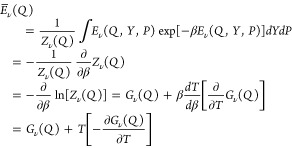A3

Thus, the thermal averaging in eq A3 leads to

A4

where

A5

is the entropy associated with the Y degrees of freedom, defined according to Planck–Boltzmann. In fact, the probability density of {Y,P} conditional on Q is

A6

and

A7

The significance of G_ν(Q) as the effective potential energy for the Q motion is seen by calculating the average force on the Q degree of freedom arising from the Y nuclear coordinates:

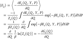A8

In eq A8, the derivative of E_ν(Q,Y,P) with respect to Q is evaluated using the Hellmann–Feynman theorem if Q represents an eigenvalue of the position operator of a quantum degree of freedom.¹¹⁴

Equation A8 shows that the free energy G_ν(Q) associated with the nonreactive environmental degrees of freedom and a given quantum state of the {q,R} subsystem act as a “potential of mean force”.^488,489 Therefore, the free energy G_ν(Q) is an effective potential for the nuclear motion along the reaction coordinate Q. Ultimately, as in ref (486) and considering the general case of more reactive coordinates, we can say that G_ν(Q) describes a “potential free energy surface” (PFES).

It is worth noting that, if the reactive electron–proton subsystem interacts significantly with the Q coordinate (which is thus identified as the reaction coordinate) while its direct interaction with Y is negligible, then the difference G_ν(Q) – G_μ(Q) for two different ν and μ electron–proton states equals their energy difference. We next illustrate this circumstance in the simpler case of pure ET.

Using familiar approximations (that is, an explicit treatment of only the transferring electron as discussed in section 5.2, i.e., a single-electron model; a quadratic expansion of the environmental degrees of freedom in the Hamiltonian; linear coupling between q and Q), the ET Hamiltonian can be written as¹⁷⁷

A9

where H^q is the one-electron Hamiltonian, H^q–Q is the electron–nucleus (q–Q) interaction energy, H^Q is the Hamiltonian for the reactive coordinate, and H^Q–Y includes the energy of Y and the Q–Y interaction energy. Substituting this Hamiltonian into the Schrödinger equation for the electronic wave function, and adding the Y kinetic energy, one obtains energy eigenvalues of the form

A10

for a given quantum state ν of the electron and a fixed value of Q. ε_ν(Q) also contains the q–Q interaction. Using eq A10, one finds that, for any two quantum states ν and μ

A11

Thus, eq A7 yields S_ν (Q) = S_μ(Q), and (assuming that the two electronic states have equal-fold degeneracy)

A12

Equation A12 expresses the fact that, in the approximations used, the electronic state does not affect the entropy of the Y subsystem for any given Q, because the electron does not appreciably interact with the nonreactive nuclear modes. As such, the PFES reduces to a “mean potential energy surface” (MPES⁴⁸⁶).

Appendix B

In this appendix, we further examine the equations of motion for the PCET system (described in terms of the nuclear wave functions associated with different electronic states in eq 5.40) using the density matrix formalism. The implications of using nonorthogonal electronic diabatic states will be discussed. We will also shed some light on the correlation properties of eq 5.39 and their relationship to graphs such as those of Figure 18. The analysis is formulated here in terms of a single nuclear reaction coordinate Q, which may be interpreted as a set of nuclear coordinates.

The state in eq 5.39 corresponds to the density operator

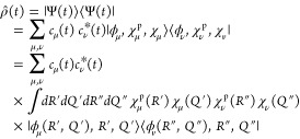B1

where the decomposition of the identity operator in the continuous basis generated by the observables R̂ and Q̂ is used to obtain the expansion in the |ϕ_n,R,Q⟩ basis. The matrix elements

B2

represent (a) the population of state |ϕ_n,R,Q⟩ at time t for k = n (namely, the probability density that at this instant the proton is at position R and the other nuclei are at Q while the electron is in state |ϕ_n⟩) and (b) the coherence between states |ϕ_k,R,Q⟩ and |ϕ_n,R,Q⟩, for k ≠ n (i.e., the coherence between the diabatic electronic states |ϕ_k⟩ and |ϕ_k⟩ in the nuclear conformation {R,Q}).

The other density matrix elements

B3

contain correlations between the conformations {R,Q} in the electronic state |ϕ_k⟩ and {R′,Q′} in the electronic state |ϕ_n⟩.

The evolution of the PCET system is described by the quantum Liouville equation

B4

Substituting eq B1 into eq B4, averaging over state |ϕ_n,R,Q⟩, and substituting eqs B2 and B3 gives (see section 4 in the Supporting Information)

B5

The same equation of motion (eq B5) is obtained by multiplying eq 5.40 on the left by χ_n^p(R)ξ_n(Q,t) and the complex conjugate of eq B1 by χ_n^p(R)ξ_n(Q,t) and finally subtracting the two resulting equations. Given the probability |c_n(t)|² that the reactive electron is in state |ϕ_n⟩ and the probability density [χ_n(R)χ_n(Q)]² that the proton–solvent subsystem is in the {R,Q} conformation at time t, the evolution of the system is described by eq B5 and depends on the ET matrix elements V_nk.

Formulating the quantum dynamics with orthogonal diabatic electronic states simplifies eqs 5.40 and B1. However, in several systems of interest the charge transfer reaction involves initial and final localized distributions of the excess electronic charge with nonzero overlap.^{134,135,144,159,490} When a nonorthogonal diabatic basis set appropriately describes the electronic structures of reactants and products, the appropriate orthogonal diabatic electronic set to be used in eqs 5.39a (or 5.39b), 5.40, and B1 needs¹⁴⁴ to be related to the nonorthogonal one by a Löwdin transformation.⁴⁹¹ Instead, when the nonorthogonal diabatic basis is used, overlaps between the diabatic electronic states appear in eq 5.40 or similar equations of motion for other kinds of charge transfer systems (for example, see ref (159) for pure ET reactions). For a reaction involving two electronic states, |ϕ_I⟩ and |ϕ_F⟩, the electronic transition is induced by the effective electronic coupling:^134,141,144

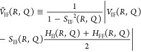B6

where S_IF = ⟨ϕ_I|ϕ_F⟩, V_IF = ⟨ϕ_I|H|ϕ_F⟩, H_II = ⟨ϕ_I|H|ϕ_I⟩, and H_FF = ⟨ϕ_F|H|ϕ_F⟩. As shown in ref (159) for a multistate ET system, replacing the electronic coupling V_IF with the effective electronic coupling Ṽ_IF allows treatment of the transition probability similarly in terms of orthogonal and nonorthogonal states (thus, extending the analysis in section 5 to nonorthogonal sets). It was also shown that, within a two-electronic state model of ET and for sufficiently small diabatic-state overlap S_IF,^144,492Ṽ_IF and V_IF can be given the same functional dependence on the electronic structure properties of the diabatic electronic states involved in the ET (even though the values of these properties depend on S_IF(95)), which facilitates the extension of the analysis of PCET in section 5 to nonorthogonal electronic diabatic representations. Note that the electronic coupling must always be (and is, as guaranteed by the Löwdin transformation) expressible in terms of orthogonal electronic states.⁴⁹³ Note also that V_IF is not independent of the arbitrary zero of the Hamiltonian when nonorthogonal diabatic electronic states are used. In this case, Ṽ_IF represents the correct expression for the coupling and is clearly independent of the zero of the energy scale.

Knowledge of the system state in terms of orthogonal or nonorthogonal electronic diabatic states affects the properties of quantum entanglement^494,495 among the relevant components: reactive electron, reactive proton, and nuclear collective coordinates. In other words, considering the system from the perspective of the quantum measurement of its properties, the investigations in terms of the orthogonal or nonorthogonal electronic basis will lead to different information regarding the system and different characterizations of its subsystems. The density matrix in eq B1 represents a pure entangled state of a tripartite system.^494,496 Therefore, (i) the system von Neumann entropy⁴⁹⁷(t) = −k_B Tr[ρ̂(t) ln ρ̂(t)] is zero irrespective of the electronic state basis used in the expansion of eq 5.39a or 5.39b, and hence in the density operator of eq B1. (ii) Only for orthogonal electronic states, the proton–solvent subsystem, unconditional on the electron subsystem, is in a separable state,^496,498 which is described by the density matrix

B7

The state described by eq B7 is characterized by classical-type correlations (in contrast, the presence of quantum entanglement can be defined by the impossibility of writing the system state in the separable form of eq B7, with the resulting unusual properties of the mutual entropy, i.e., of the information gained about one subsystem by measurement on the other subsystem⁴⁹⁵). This absence of quantum entanglement between the R and Q subsystems for a given electronic state, together with the condition of small nonadiabatic coupling between the proton and solvent dynamics, justifies the use of the second adiabatic approximation. In turn, the application of the second adiabatic approximation leads to free energy landscapes for ensembles of system states as shown in Figure 18.⁴⁹⁵

Supporting Information Available

Figures S1–S9 showing stereo views of the protein environments surrounding Tyr161 (TyrZ) and Tyr160 (TyrD) of photosystem II from T. vulcanus, Tyr8 of the BLUF domain from Slr1694 of Synechocystis sp. PCC 6803, Tyr122 and Trp48 of ribonucleotide reductase from E. coli, Trp382 and Trp306 of photolyase from E. coli, and Trp122 of azurin from P. aeruginosa and a side by side comparison of the protein environments surrounding D1-Tyr161 (TyrZ) and D2-Tyr160 (TyrD) of photosystem II from T. vulcanus and derivations of eqs 5.18, 5.21, 6.9a, 6.9b, 6.10, and B5. This material is available free of charge via the Internet at http://pubs.acs.org.

The authors declare no competing financial interest.

Funding Statement

National Institutes of Health, United States

References

- Liu Z.; Tan C.; Guo X.; Li J.; Wang L.; Sancar A.; Zhong D. Proc. Natl. Acad. Sci. U.S.A. 2013, 110, 12966. [DOI] [PMC free article] [PubMed] [Google Scholar]
- Kaila V. R. I.; Verkhovsky M. I.; Wikström M. Chem. Rev. 2010, 110, 7062. [DOI] [PubMed] [Google Scholar]
- Hino T.; Matsumoto Y.; Nagano S.; Sugimoto H.; Fukumori Y.; Murata T.; Iwata S.; Shiro Y. Science 2010, 330, 1666. [DOI] [PubMed] [Google Scholar]
- Weinberg D. R.; Gagliardi C. J.; Hull J. F.; Murphy C. F.; Kent C. A.; Westlake B. C.; Paul A.; Ess D. H.; McCafferty D. G.; Meyer T. J. Chem. Rev. 2012, 112, 4016. [DOI] [PubMed] [Google Scholar]
- Smith K. W.; Stroupe M. E. Biochemistry 2012, 51, 9857. [DOI] [PubMed] [Google Scholar]
- Kennis J. T. M.; Mathes T. Interface Focus 2013, 3, 20130005. [DOI] [PMC free article] [PubMed] [Google Scholar]
- Marcus R. A.; Sutin N. Biochim. Biophys. Acta, Rev. Bioenerg. 1985, 811, 265. [Google Scholar]
- Beratan D. N.; Onuchic J. N.; Winkler J. R.; Gray H. B. Science 1992, 258, 1740. [DOI] [PubMed] [Google Scholar]
- Dempsey J. L.; Winkler J. R.; Gray H. B. Chem. Rev. 2010, 110, 7024. [DOI] [PMC free article] [PubMed] [Google Scholar]
- Harriman A. J. Phys. Chem. 1987, 91, 6102. [Google Scholar]
- Aubert C.; Mathis P.; Eker A. P. M.; Brettel K. Proc. Natl. Acad. Sci. U.S.A. 1999, 96, 5423. [DOI] [PMC free article] [PubMed] [Google Scholar]
- Rappaport F.; Boussac A.; Force D. A.; Peloquin J.; Brynda M.; Sugiura M.; Un S.; Britt R. D.; Diner B. A. J. Am. Chem. Soc. 2009, 131, 4425. [DOI] [PMC free article] [PubMed] [Google Scholar]
- Mathes T.; Zhu J.; van Stokkum I. H. M.; Groot M. L.; Hegemann P.; Kennis J. T. M. J. Phys. Chem. Lett. 2012, 3, 203. [Google Scholar]
- Aubert C.; Vos M. H.; Mathis P.; Eker A. P. M.; Brettel K. Nature 2000, 405, 586. [DOI] [PubMed] [Google Scholar]
- Hibbert F.; Emsley J. In Advances in Physical Organic Chemistry; Bethell D., Ed.; Academic Press: New York, 1991; Vol. 26. [Google Scholar]
- Perrin C. L.; Nielson J. B. Annu. Rev. Phys. Chem. 1997, 48, 511. [DOI] [PubMed] [Google Scholar]
- Fuhrmann C. N.; Daugherty M. D.; Agard D. A. J. Am. Chem. Soc. 2006, 128, 9086. [DOI] [PubMed] [Google Scholar]
- Frey P. A.; Whitt S. A.; Tobin J. B. Science 1994, 264, 1927. [DOI] [PubMed] [Google Scholar]
- Saito K.; Shen J.-R.; Ishida T.; Ishikita H. Biochemistry 2011, 50, 9836. [DOI] [PubMed] [Google Scholar]
- Zhang C. Biochim. Biophys. Acta, Bioenerg. 2007, 1767, 493. [DOI] [PubMed] [Google Scholar]
- Umena Y.; Kawakami K.; Shen J.-R.; Kamiya N. Nature 2011, 473, 55. [DOI] [PubMed] [Google Scholar]
- Frey P. A. J. Phys. Org. Chem. 2004, 17, 511. [Google Scholar]
- Cleland W. W.; Kreevoy M. M. Science 1994, 264, 1887. [DOI] [PubMed] [Google Scholar]
- Yamaguchi S.; Kamikubo H.; Kurihara K.; Kuroki R.; Niimura N.; Shimizu N.; Yamazaki Y.; Kataoka M. Proc. Natl. Acad. Sci. U.S.A. 2009, 106, 440. [DOI] [PMC free article] [PubMed] [Google Scholar]
- Saito K.; Ishikita H. Proc. Natl. Acad. Sci. U.S.A. 2012, 109, 167. [DOI] [PMC free article] [PubMed] [Google Scholar]
- Saito K.; Rutherford A. W.; Ishikita H. Proc. Natl. Acad. Sci. U.S.A. 2013, 110, 7690. [DOI] [PMC free article] [PubMed] [Google Scholar]
- Chatterjee R.; Coates C. S.; Milikisiyants S.; Lee C.-I.; Wagner A.; Poluektov O. G.; Lakshmi K. V. Biochemistry 2013, 52, 4781. [DOI] [PubMed] [Google Scholar]
- Offenbacher A. R.; Burns L. A.; Sherrill C. D.; Barry B. A. J. Phys. Chem. B 2013, 117, 8457. [DOI] [PMC free article] [PubMed] [Google Scholar]
- Jeffrey G. A.An Introduction to Hydrogen Bonding; Oxford University Press: New York, 1997. [Google Scholar]
- Golan A.; Bravaya K. B.; Kudirka R.; Kostko O.; Leone S. R.; Krylov A. I.; Ahmed M. Nat. Chem. 2012, 4, 323. [DOI] [PubMed] [Google Scholar]
- Ishikita H.; Saito K. J. R. Soc. Interface 2014, 11, 20130518. [DOI] [PMC free article] [PubMed] [Google Scholar]
- Mayer J. M.; Hrovat D. A.; Thomas J. L.; Borden W. T. J. Am. Chem. Soc. 2002, 124, 11142. [DOI] [PubMed] [Google Scholar]
- Inagaki T.; Yamamoto T.; Kato S. J. Comput. Chem. 2011, 32, 3081. [DOI] [PubMed] [Google Scholar]
- Vinyard D. J.; Ananyev G. M.; Charles Dismukes G. Annu. Rev. Biochem. 2013, 82, 577. [DOI] [PubMed] [Google Scholar]
- Minnihan E. C.; Nocera D. G.; Stubbe J. Acc. Chem. Res. 2013, 46, 2524. [DOI] [PMC free article] [PubMed] [Google Scholar]
- Stubbe J.; Nocera D. G.; Yee C. S.; Chang M. C. Chem. Rev. 2003, 103, 2167. [DOI] [PubMed] [Google Scholar]
- Whittaker J. W. Chem. Rev. 2003, 103, 2347. [DOI] [PubMed] [Google Scholar]
- Styring S.; Sjöholm J.; Mamedov F. Biochim. Biophys. Acta, Bioenerg. 2012, 1817, 76. [DOI] [PubMed] [Google Scholar]
- Magnuson A.; Berglund H.; Korall P.; Hammarström L.; Åkermark B.; Styring S.; Sun L. J. Am. Chem. Soc. 1997, 119, 10720. [Google Scholar]
- Irebo T.; Reece S. Y.; Sjödin M.; Nocera D. G.; Hammarström L. J. Am. Chem. Soc. 2007, 129, 15462. [DOI] [PubMed] [Google Scholar]
- Abrahamsson M. L. A.; Baudin H. B.; Tran A.; Philouze C.; Berg K. E.; Raymond-Johansson M. K.; Sun L.; Åkermark B.; Styring S.; Hammarström L. Inorg. Chem. 2002, 41, 1534. [DOI] [PubMed] [Google Scholar]
- Sun L.; Raymond M. K.; Magnuson A.; LeGourrierec D.; Tamm M.; Abrahamsson M.; Kenéz P. H.; Mårtensson J.; Stenhagen G.; Hammarström L.; Styring S.; Åkermark B. J. Inorg. Biochem. 2000, 78, 15. [DOI] [PubMed] [Google Scholar]
- Saito K.; Rutherford A. W.; Ishikita H. Proc. Natl. Acad. Sci. U.S.A. 2013, 110, 954. [DOI] [PMC free article] [PubMed] [Google Scholar]
- Meyer T. J.; Huynh M. H. V.; Thorp H. H. Angew. Chem., Int. Ed. 2007, 46, 5284. [DOI] [PubMed] [Google Scholar]
- Wynne K.; LeCours S. M.; Galli C.; Therien M. J.; Hochstrasser R. M. J. Am. Chem. Soc. 1995, 117, 3749. [Google Scholar]
- Kang Y. K.; Rubtsov I. V.; Iovine P. M.; Chen J.; Therien M. J. J. Am. Chem. Soc. 2002, 124, 8275. [DOI] [PubMed] [Google Scholar]
- Wasielewski M. R. Chem. Rev. 1992, 92, 435. [Google Scholar]
- Joran A. D.; Leland B. A.; Geller G. G.; Hopfield J. J.; Dervan P. B. J. Am. Chem. Soc. 1984, 106, 6090. [Google Scholar]
- Megiatto J. D.; Antoniuk-Pablant A.; Sherman B. D.; Kodis G.; Gervaldo M.; Moore T. A.; Moore A. L.; Gust D. Proc. Natl. Acad. Sci. U.S.A. 2012, 109, 15578. [DOI] [PMC free article] [PubMed] [Google Scholar]
- Irebo T.; Zhang M.-T.; Markle T. F.; Scott A. M.; Hammarström L. J. Am. Chem. Soc. 2012, 134, 16247. [DOI] [PubMed] [Google Scholar]
- Chen G.; Han G.; Göransson E.; Mamedov F.; Styring S. Biochemistry 2011, 51, 138. [DOI] [PubMed] [Google Scholar]
- Dau H.; Zaharieva I. Acc. Chem. Res. 2009, 42, 1861. [DOI] [PubMed] [Google Scholar]
- Fleming G. R.; van Grondelle R. Phys. Today 1994, 47, 48. [Google Scholar]
- PyMol; Schrodinger, LLC: Portland, OR, 2010. [Google Scholar]
- Faries K. M.; Kressel L. L.; Wander M. J.; Holten D.; Laible P. D.; Kirmaier C.; Hanson D. K. J. Biol. Chem. 2012, 287, 8507. [DOI] [PMC free article] [PubMed] [Google Scholar]
- Kless H.; Vermaas W. Biochemistry 1996, 35, 16458. [DOI] [PubMed] [Google Scholar]
- Hays A.-M. A.; Vassiliev I. R.; Golbeck J. H.; Debus R. J. Biochemistry 1998, 37, 11352. [DOI] [PubMed] [Google Scholar]
- Bao H.; Dilbeck P.; Burnap R. Photosynth. Res. 2013, 116, 215. [DOI] [PubMed] [Google Scholar]
- Faller P.; Rutherford A. W.; Debus R. J. Biochemistry 2002, 41, 12914. [DOI] [PubMed] [Google Scholar]
- Rutherford A. W.; Boussac A.; Faller P. Biochim. Biophys. Acta, Bioenerg. 2004, 1655, 222. [DOI] [PubMed] [Google Scholar]
- Sjödin M.; Styring S.; Wolpher H.; Xu Y.; Sun L.; Hammarström L. J. Am. Chem. Soc. 2005, 127, 3855. [DOI] [PubMed] [Google Scholar]
- Faller P.; Debus R. J.; Brettel K.; Sugiura M.; Rutherford A. W.; Boussac A. Proc. Natl. Acad. Sci. U.S.A. 2001, 98, 14368. [DOI] [PMC free article] [PubMed] [Google Scholar]
- Takahashi R.; Sugiura M.; Noguchi T. Biochemistry 2007, 46, 14245. [DOI] [PubMed] [Google Scholar]
- Keßen S.; Teutloff C.; Kern J.; Zouni A.; Bittl R. ChemPhysChem 2010, 11, 1275. [DOI] [PubMed] [Google Scholar]
- Jenson D. L.; Barry B. A. J. Am. Chem. Soc. 2009, 131, 10567. [DOI] [PMC free article] [PubMed] [Google Scholar]
- Koua F. H. M.; Umena Y.; Kawakami K.; Shen J.-R. Proc. Natl. Acad. Sci. U.S.A. 2013, 110, 3889. [DOI] [PMC free article] [PubMed] [Google Scholar]
- Bonin J.; Costentin C.; Louault C.; Robert M.; Savéant J.-M. J. Am. Chem. Soc. 2011, 133, 6668. [DOI] [PubMed] [Google Scholar]
- Khrenova M. G.; Nemukhin A. V.; Domratcheva T. J. Phys. Chem. B 2013, 117, 2369. [DOI] [PubMed] [Google Scholar]
- Gauden M.; van Stokkum I. H. M.; Key J. M.; Lührs D. C.; van Grondelle R.; Hegemann P.; Kennis J. T. M. Proc. Natl. Acad. Sci. U.S.A. 2006, 103, 10895. [DOI] [PMC free article] [PubMed] [Google Scholar]
- Udvarhelyi A.; Domratcheva T. J. Phys. Chem. B 2013, 117, 2888. [DOI] [PubMed] [Google Scholar]
- Ishikita H. J. Biol. Chem. 2008, 283, 30618. [DOI] [PMC free article] [PubMed] [Google Scholar]
- Bonetti C.; Stierl M.; Mathes T.; van Stokkum I. H. M.; Mullen K. M.; Cohen-Stuart T. A.; van Grondelle R.; Hegemann P.; Kennis J. T. M. Biochemistry 2009, 48, 11458. [DOI] [PubMed] [Google Scholar]
- Mathes T.; van Stokkum I. H. M.; Stierl M.; Kennis J. T. M. J. Biol. Chem. 2012, 287, 31725. [DOI] [PMC free article] [PubMed] [Google Scholar]
- Offenbacher A. R.; Minnihan E. C.; Stubbe J.; Barry B. A. J. Am. Chem. Soc. 2013, 135, 6380. [DOI] [PMC free article] [PubMed] [Google Scholar]
- Han W.-G.; Noodleman L. Inorg. Chem. 2011, 50, 2302. [DOI] [PMC free article] [PubMed] [Google Scholar]
- Baldwin J.; Krebs C.; Ley B. A.; Edmondson D. E.; Huynh B. H.; Bollinger J. M. Jr. J. Am. Chem. Soc. 2000, 122, 12195. [Google Scholar]
- Bollinger J. M. Jr.; Tong W. H.; Ravi N.; Huynh B. H.; Edmonson D. E.; Stubbe J. J. Am. Chem. Soc. 1994, 116, 8015. [Google Scholar]
- Wörsdörfer B.; Conner D. A.; Yokoyama K.; Livada J.; Seyedsayamdost M.; Jiang W.; Silakov A.; Stubbe J.; Bollinger J. M.; Krebs C. J. Am. Chem. Soc. 2013, 135, 8585. [DOI] [PMC free article] [PubMed] [Google Scholar]
- Minnihan E. C.; Ando N.; Brignole E. J.; Olshansky L.; Chittuluru J.; Asturias F. J.; Drennan C. L.; Nocera D. G.; Stubbe J. Proc. Natl. Acad. Sci. U.S.A. 2013, 110, 3835. [DOI] [PMC free article] [PubMed] [Google Scholar]
- Yokoyama K.; Uhlin U.; Stubbe J. J. Am. Chem. Soc. 2010, 132, 15368. [DOI] [PMC free article] [PubMed] [Google Scholar]
- Barry B. A.; Chen J.; Keough J.; Jenson D.; Offenbacher A.; Pagba C. J. Phys. Chem. Lett. 2012, 3, 543. [DOI] [PMC free article] [PubMed] [Google Scholar]
- Högbom M.; Galander M.; Andersson M.; Kolberg M.; Hofbauer W.; Lassmann G.; Nordlund P.; Lendzian F. Proc. Natl. Acad. Sci. U.S.A. 2003, 100, 3209. [DOI] [PMC free article] [PubMed] [Google Scholar]
- Yokoyama K.; Uhlin U.; Stubbe J. J. Am. Chem. Soc. 2010, 132, 8385. [DOI] [PMC free article] [PubMed] [Google Scholar]
- Tommos C.; Babcock G. T. Biochim. Biophys. Acta, Bioenerg. 2000, 1458, 199. [DOI] [PubMed] [Google Scholar]
- Silva K. E.; Elgren T. E.; Que L.; Stankovich M. T. Biochemistry 1995, 34, 14093. [DOI] [PubMed] [Google Scholar]
- Xue G.; De Hont R.; Münck E.; Que L. Nat. Chem. 2010, 2, 400. [DOI] [PMC free article] [PubMed] [Google Scholar]
- Zieba A. A.; Richardson C.; Lucero C.; Dieng S. D.; Gindt Y. M.; Schelvis J. P. M. J. Am. Chem. Soc. 2011, 133, 7824. [DOI] [PubMed] [Google Scholar]
- Shih C.; Museth A. K.; Abrahamsson M.; Blanco-Rodriguez A. M.; Di Bilio A. J.; Sudhamsu J.; Crane B. R.; Ronayne K. L.; Towrie M.; Vlček A.; Richards J. H.; Winkler J. R.; Gray H. B. Science 2008, 320, 1760. [DOI] [PubMed] [Google Scholar]
- Blanco-Rodríguez A. M.; Di Bilio A. J.; Shih C.; Museth A. K.; Clark I. P.; Towrie M.; Cannizzo A.; Sudhamsu J.; Crane B. R.; Sýkora J.; Winkler J. R.; Gray H. B.; Záliš S.; Vlček A. Chem. Eur. J. 2011, 17, 5350. [DOI] [PMC free article] [PubMed] [Google Scholar]
- Sancar A. Chem. Rev. 2003, 103, 2203. [DOI] [PubMed] [Google Scholar]
- Jiang N.; Kuznetsov A.; Nocek J. M.; Hoffman B. M.; Crane B. R.; Hu X.; Beratan D. N. J. Phys. Chem. B 2013, 117, 9129. [DOI] [PMC free article] [PubMed] [Google Scholar]
- Sivaraja M.; Goodin D.; Smith M.; Hoffman B. Science 1989, 245, 738. [DOI] [PubMed] [Google Scholar]
- Priyadarshy S.; Risser S. M.; Beratan D. N. J. Phys. Chem. 1996, 100, 17678. [Google Scholar]
- Genereux J. C.; Barton J. K. Chem. Rev. 2009, 110, 1642. [DOI] [PMC free article] [PubMed] [Google Scholar]
- Senthilkumar K.; Grozema F. C.; Guerra C. F.; Bickelhaupt F. M.; Lewis F. D.; Berlin Y. A.; Ratner M. A.; Siebbeles L. D. A. J. Am. Chem. Soc. 2005, 127, 14894. [DOI] [PubMed] [Google Scholar]
- Wagenknecht H.-A.; Rajski S. R.; Pascaly M.; Stemp E. D. A.; Barton J. K. J. Am. Chem. Soc. 2001, 123, 4400. [DOI] [PubMed] [Google Scholar]
- Krebs C.; Chen S.; Baldwin J.; Ley B. A.; Patel U.; Edmondson D. E.; Huynh B. H.; Bollinger J. M. Jr. J. Am. Chem. Soc. 2000, 122, 12207. [Google Scholar]
- Cotruvo J. A.; Stich T. A.; Britt R. D.; Stubbe J. J. Am. Chem. Soc. 2013, 135, 4027. [DOI] [PMC free article] [PubMed] [Google Scholar]
- Saleh L.; Bollinger J. M. Jr. Biochemistry 2006, 45, 8823. [DOI] [PubMed] [Google Scholar]
- Yokoyama K.; Smith A. A.; Corzilius B.; Griffin R. G.; Stubbe J. J. Am. Chem. Soc. 2011, 133, 18420. [DOI] [PMC free article] [PubMed] [Google Scholar]
- Ekberg M.; Pötsch S.; Sandin E.; Thunnissen M.; Nordlund P.; Sahlin M.; Sjöberg B.-M. J. Biol. Chem. 1998, 273, 21003. [DOI] [PubMed] [Google Scholar]
- Nordlund P.; Eklund H. J. Mol. Biol. 1993, 232, 123. [DOI] [PubMed] [Google Scholar]
- Balland V.; Byrdin M.; Eker A. P. M.; Ahmad M.; Brettel K. J. Am. Chem. Soc. 2009, 131, 426. [DOI] [PubMed] [Google Scholar]
- Cashmore A. R.; Jarillo J. A.; Wu Y.-J.; Liu D. Science 1999, 284, 760. [DOI] [PubMed] [Google Scholar]
- Arents J. C.; Perez M. A.; Hendriks J.; Hellingwerf K. J. FEBS Lett. 2011, 585, 167. [DOI] [PubMed] [Google Scholar]
- Warren J. J.; Ener M. E.; Vlček A. Jr; Winkler J. R.; Gray H. B. Coord. Chem. Rev. 2012, 256, 2478. [DOI] [PMC free article] [PubMed] [Google Scholar]
- Gray H. B. Chem. Soc. Rev. 1986, 15, 17. [Google Scholar]
- Langen R.; Chang I. J.; Germanas J. P.; Richards J. H.; Winkler J. R.; Gray H. B. Science 1995, 268, 1733. [DOI] [PubMed] [Google Scholar]
- Gray H. B.; Winkler J. R. Q. Rev. Biophys. 2003, 36, 341. [DOI] [PubMed] [Google Scholar]
- Renger G.; Renger T. Photosynth. Res. 2008, 98, 53. [DOI] [PubMed] [Google Scholar]
- Bender G. M.; Lehmann A.; Zou H.; Cheng H.; Fry H. C.; Engel D.; Therien M. J.; Blasie J. K.; Roder H.; Saven J. G.; DeGrado W. F. J. Am. Chem. Soc. 2007, 129, 10732. [DOI] [PMC free article] [PubMed] [Google Scholar]
- Fry H. C.; Lehmann A.; Saven J. G.; DeGrado W. F.; Therien M. J. J. Am. Chem. Soc. 2010, 132, 3997. [DOI] [PMC free article] [PubMed] [Google Scholar]
- Fry H. C.; Lehmann A.; Sinks L. E.; Asselberghs I.; Tronin A.; Krishnan V.; Blasie J. K.; Clays K.; DeGrado W. F.; Saven J. G.; Therien M. J. J. Am. Chem. Soc. 2013, 135, 13914. [DOI] [PMC free article] [PubMed] [Google Scholar]
- Weissbluth M.Atoms and Molecules; Academic Press: New York, 1978. [Google Scholar]
- Born M.; Oppenheimer R. Ann. Phys. (Berlin) 1927, 84, 457. [Google Scholar]
- Cukier R. I. J. Phys. Chem. 1995, 99, 16101. [Google Scholar]
- Bransden B. H.; Joachain C. J.. Physics of Atoms and Molecules; John Wiley & Sons: New York, 1988. [Google Scholar]
- Born M.; Fock V. A. Z. Phys. 1928, 51, 165. [Google Scholar]
- Tully J. C. J. Chem. Phys. 1990, 93, 1061. [Google Scholar]
- Shenvi N.; Roy S.; Tully J. C. J. Chem. Phys. 2009, 130, 174107. [DOI] [PubMed] [Google Scholar]
- Cohen-Tannoudji C.; Diu B.; Laloë F.. Quantum Mechanics; Hermann: Paris, 1977. [Google Scholar]
- Marcus R. A. Annu. Rev. Phys. Chem. 1964, 15, 155. [Google Scholar]
- Domcke W.; Yarkony D. R. Annu. Rev. Phys. Chem. 2012, 63, 325. [DOI] [PubMed] [Google Scholar]
- Hobey W. D.; McLachlan A. D. J. Chem. Phys. 1960, 33, 1695. [Google Scholar]
- Mikkelsen K. V.; Ratner M. A. Chem. Rev. 1987, 87, 113. [Google Scholar]
- Kuznetsov A. M.; Ulstrup J.; Vorotyntsev M. A.. Solvent Effects in Charge Transfer Processes. In The Chemical Physics of Solvation, Part C; Elsevier Science Publishers B.V.: Amsterdam, 1988. [Google Scholar]
- Newton M. D.; Sutin N. Annu. Rev. Phys. Chem. 1984, 35, 437. [Google Scholar]
- Mead C. A.; Truhlar D. G. J. Chem. Phys. 1982, 77, 6090. [Google Scholar]
- Cederbaum L. S. J. Chem. Phys. 1983, 78, 5714. [Google Scholar]
- Kryachko E. S.; Yarkony D. R. Int. J. Quantum Chem. 2000, 76, 235. [Google Scholar]
- Nakamura H.; Truhlar D. G. J. Chem. Phys. 2001, 115, 10353. [Google Scholar]
- Worth G. A.; Robb M. A.; Lasorne B. Mol. Phys. 2008, 106, 2077. [Google Scholar]
- Pavanello M.; Neugebauer J. J. Chem. Phys. 2011, 135, 134113. [DOI] [PubMed] [Google Scholar]
- Farazdel A.; Dupuis M.; Clementi E.; Aviram A. J. Am. Chem. Soc. 1990, 112, 4206. [Google Scholar]
- Newton M. D. Chem. Rev. 1991, 91, 767. [Google Scholar]
- Wesolowski T. A.; Warshel A. J. Phys. Chem. 1993, 97, 8050. [Google Scholar]
- Kamerlin S. C. L.; Vicatos S.; Dryga A.; Warshel A. Annu. Rev. Phys. Chem. 2011, 62, 41. [DOI] [PubMed] [Google Scholar]
- Voityuk A. A.; Rösch N. J. Chem. Phys. 2002, 117, 5607. [Google Scholar]
- Song L. C.; Gao J. L. J. Phys. Chem. A 2008, 112, 12925. [DOI] [PMC free article] [PubMed] [Google Scholar]
- Subotnik J. E.; Cave R. J.; Steele R. P.; Shenvi N. J. Chem. Phys. 2009, 130, 234102. [DOI] [PubMed] [Google Scholar]
- Migliore A. J. Chem. Phys. 2009, 131, 114113. [DOI] [PMC free article] [PubMed] [Google Scholar]
- Cave R. J.; Edwards S. T.; Kouzelos J. A.; Newton M. D. J. Phys. Chem. B 2010, 114, 14631. [DOI] [PubMed] [Google Scholar]
- Van Voorhis T.; Kowalczyk T.; Kaduk B.; Wang L.-P.; Cheng C.-L.; Wu Q. Annu. Rev. Phys. Chem. 2010, 61, 149. [DOI] [PubMed] [Google Scholar]
- Migliore A. J. Chem. Theory Comput. 2011, 7, 1712. [DOI] [PubMed] [Google Scholar]
- Pavanello M.; Van Voorhis T.; Visscher L.; Neugebauer J. J. Chem. Phys. 2013, 138, 054101. [DOI] [PubMed] [Google Scholar]
- Blumberger J.; McKenna K. P. Phys. Chem. Chem. Phys. 2013, 15, 2184. [DOI] [PubMed] [Google Scholar]
- Marcus R. A. J. Chem. Phys. 1956, 24, 966. [Google Scholar]
- Marcus R. A. J. Chem. Phys. 1956, 24, 979. [Google Scholar]
- Nitzan A.Chemical Dynamics in Condensed Phases; Oxford University Press: Oxford, U.K., 2007. [Google Scholar]
- Marcus R. A. Rev. Mod. Phys. 1993, 65, 599. [Google Scholar]
- Small D. W.; Matyushov D. V.; Voth G. A. J. Am. Chem. Soc. 2003, 125, 7470. [DOI] [PubMed] [Google Scholar]
- Levich V. G.; Dogonadze R. R. Dokl. Akad. Nauk SSSR 1959, 124, 123. [Google Scholar]
- Levich V. G.; Dogonadze R. R. Dokl. Akad. Nauk SSSR 1960, 133, 158. [Google Scholar]
- Landau L. D. Phys. Z. Sowjetunion 1932, 1, 88. [Google Scholar]
- Landau L. D. Phys. Z. Sowjetunion 1932, 2, 46. [Google Scholar]
- Zener C. Proc. R. Soc. London, A 1932, 137, 696. [Google Scholar]
- Zener C. Proc. R. Soc. London, A 1933, 140, 660. [Google Scholar]
- Kubo R.; Toyozawa Y. Prog. Theor. Phys. 1955, 13, 160. [Google Scholar]
- Kuznetsov A. M.; Ulstrup J.. Electron Transfer in Chemistry and Biology; John Wiely & Sons: New York, 1999. [Google Scholar]
- Morelli J.; Hammes-Schiffer S. Chem. Phys. Lett. 1997, 269, 161. [Google Scholar]
- Peube J.-L.Fundamentals of Fluid Mechanics and Transport Phenomena; Wiley: Hoboken, NJ, 2009. [Google Scholar]
- Ulstrup J.Lecture Notes in Chemistry; Springer-Verlag: Berlin, 1979. [Google Scholar]
- Baer M. Phys. Rep. 2002, 358, 75. [Google Scholar]
- Sirjoosingh A.; Hammes-Schiffer S. J. Phys. Chem. A 2011, 115, 2367. [DOI] [PubMed] [Google Scholar]
- Borgis D.; Hynes J. T. J. Chem. Phys. 1991, 94, 3619. [Google Scholar]
- Borgis D.; Tarjus G.; Azzouz H. J. Phys. Chem. 1992, 96, 3188. [Google Scholar]
- Hammes-Schiffer S.; Tully J. C. J. Chem. Phys. 1994, 101, 4657. [Google Scholar]
- Fukui K. J. Phys. Chem. 1970, 74, 4161. [Google Scholar]
- Moore J. W.; Pearson R. G.. Kinetics and Mechanism, 3rd ed.; John Wiley & Sons, Inc.: New York, 1981. [Google Scholar]
- Fukui K. Acc. Chem. Res. 1981, 14, 363. [Google Scholar]
- Deng L. Q.; Ziegler T. Int. J. Quantum Chem. 1994, 52, 731. [Google Scholar]
- Okuno Y. J. Chem. Phys. 1999, 111, 8034. [Google Scholar]
- Allison T. C.; Lynch G. C.; Truhlar D. G.; Gordon M. S. J. Phys. Chem. 1996, 100, 13575. [Google Scholar]
- Truhlar D. G.; Mead C. A. Phys. Rev. A 2003, 68, 032501. [Google Scholar]
- Tishchenko O.; Truhlar D. G.; Ceulemans A.; Nguyen M. T. J. Am. Chem. Soc. 2008, 130, 7000. [DOI] [PubMed] [Google Scholar]
- Sakurai J. J.Modern Quantum Mechanics, rev. ed.; Addison-Wesley Publishing Co., Inc.: New York, 1994; p 477. [Google Scholar]
- Onuchic J. N.; Beratan D. N.; Hopfield J. J. J. Phys. Chem. 1986, 90, 3707. [Google Scholar]
- Dogonadze R. R.; Kuznetsov A. M.; Levich V. G. Elektrokhimiya 1967, 3, 739. [Google Scholar]
- Dogonadze R. R.; Kuznetsov A. M.; Levich V. G. Electrochim. Acta 1968, 13, 1025. [Google Scholar]
- Levich V. G.; Dogonadze R. R.; German E. D.; Kuznetsov A. M.; Kharkats Y. I. Electrochim. Acta 1970, 15, 353. [Google Scholar]
- Kuznetsov A. M.; Ulstrup J. Can. J. Chem. 1999, 77, 1085. [Google Scholar]
- Hammes-Schiffer S. Energy Environ. Sci. 2012, 5, 7696. [Google Scholar]
- Kuznetsov A. M.; Ulstrup J. Russ. J. Electrochem. 2003, 39, 9. [Google Scholar]
- Hammes-Schiffer S.; Stuchebrukhov A. A. Chem. Rev. 2010, 110, 6939. [DOI] [PMC free article] [PubMed] [Google Scholar]
- Koper M. T. M. Phys. Chem. Chem. Phys. 2013, 15, 1399. [DOI] [PubMed] [Google Scholar]
- Kretchmer J. S.; Miller T. F. J. Chem. Phys. 2013, 138, 134109. [DOI] [PubMed] [Google Scholar]
- Cukier R. I. J. Phys. Chem. 1994, 98, 2377. [Google Scholar]
- Cukier R. I. J. Phys. Chem. 1996, 100, 15428. [Google Scholar]
- Cukier R. I.; Nocera D. G. Annu. Rev. Phys. Chem. 1998, 49, 337. [DOI] [PubMed] [Google Scholar]
- Cukier R. I. J. Phys. Chem. B 2002, 106, 1746. [Google Scholar]
- Soudackov A.; Hammes-Schiffer S. J. Chem. Phys. 2000, 113, 2385. [Google Scholar]
- Borgis D. C.; Lee S. Y.; Hynes J. T. Chem. Phys. Lett. 1989, 162, 19. [Google Scholar]
- Borgis D.; Hynes J. T. Chem. Phys. 1993, 170, 315. [Google Scholar]
- Hammes-Schiffer S. Acc. Chem. Res. 2001, 34, 273. [DOI] [PubMed] [Google Scholar]
- Georgievskii Y.; Stuchebrukhov A. A. J. Chem. Phys. 2000, 113, 10438. [Google Scholar]
- Iordanova N.; Decornez H.; Hammes-Schiffer S. J. Am. Chem. Soc. 2001, 123, 3723. [DOI] [PubMed] [Google Scholar]
- Skone J. H.; Soudackov A. V.; Hammes-Schiffer S. J. Am. Chem. Soc. 2006, 128, 16655. [DOI] [PubMed] [Google Scholar]
- Gamow G. Z. Phys. 1928, 51, 204. [Google Scholar]
- Wentzel G. Z. Phys. 1926, 38, 518. [Google Scholar]
- Kramers H. A. Z. Phys. 1926, 39, 828. [Google Scholar]
- Brillouin L. Comptes Rendus 1926, 183, 24. [Google Scholar]
- Schiff L. I.Quantum Mechanics; McGraw-Hill Book Co., Inc.: York, PA, 1949. [Google Scholar]
- Reece S. Y.; Hodgkiss J. M.; Stubbe J.; Nocera D. G. Philos. Trans. R. Soc., B 2006, 361, 1351. [DOI] [PMC free article] [PubMed] [Google Scholar]
- Reece S. Y.; Seyedsayamdost M. R.; Stubbe J.; Nocera D. G. J. Am. Chem. Soc. 2006, 128, 13654. [DOI] [PubMed] [Google Scholar]
- Sharpe M. A.; Ferguson-Miller S. J. Bioenerg. Biomembr. 2008, 40, 541. [DOI] [PMC free article] [PubMed] [Google Scholar]
- Kaila V. R. I.; Johansson M. P.; Sundholm D.; Laakkonen L.; Wikström M. Biochim. Biophys. Acta, Bioenerg. 2009, 1787, 221. [DOI] [PubMed] [Google Scholar]
- Lukacs A.; Eker A. P. M.; Byrdin M.; Brettel K.; Vos M. H. J. Am. Chem. Soc. 2008, 130, 14394. [DOI] [PubMed] [Google Scholar]
- Langenbacher T.; Immeln D.; Dick B.; Kottke T. J. Am. Chem. Soc. 2009, 131, 14274. [DOI] [PubMed] [Google Scholar]
- Nam W. Acc. Chem. Res. 2007, 40, 522. [DOI] [PubMed] [Google Scholar]
- Sugimoto H.; Tsukube H. Chem. Soc. Rev. 2008, 37, 2609. [DOI] [PubMed] [Google Scholar]
- Rajapakshe A.; Snyder R. A.; Astashkin A. V.; Bernardson P.; Evans D. J.; Young C. G.; Evans D. H.; Enemark J. H. Inorg. Chim. Acta 2009, 362, 4603. [DOI] [PMC free article] [PubMed] [Google Scholar]
- Chen Z. F.; Concepcion J. J.; Luo H. L.; Hull J. F.; Paul A.; Meyer T. J. J. Am. Chem. Soc. 2010, 132, 17670. [DOI] [PubMed] [Google Scholar]
- Wenger O. S. Acc. Chem. Res. 2013, 46, 1517. [DOI] [PubMed] [Google Scholar]
- Soudackov A.; Hammes-Schiffer S. J. Chem. Phys. 1999, 111, 4672. [Google Scholar]
- Hammes-Schiffer S.; Soudackov A. V. J. Phys. Chem. B 2008, 112, 14108. [DOI] [PMC free article] [PubMed] [Google Scholar]
- Warshel A. J. Phys. Chem. 1982, 86, 2218. [Google Scholar]
- Calef D. F.; Wolynes P. G. J. Phys. Chem. 1983, 87, 3387. [Google Scholar]
- Morse P. M.Thermal Physics; Benjamin: New York, 1964. [Google Scholar]
- Krishtalik L. I. Biochim. Biophys. Acta, Bioenerg. 2000, 1458, 6. [DOI] [PubMed] [Google Scholar]
- Hammes-Schiffer S. ChemPhysChem 2002, 3, 33. [DOI] [PubMed] [Google Scholar]
- Hammes-Schiffer S. Acc. Chem. Res. 2006, 39, 93. [DOI] [PubMed] [Google Scholar]
- Zusman L. D. Chem. Phys. 1980, 49, 295. [Google Scholar]
- Landauer R.; Martin T. Rev. Mod. Phys. 1994, 66, 217. [Google Scholar]
- Merzbacher E.Quantum Mechanics, 3rd ed.; John Wiley & Sons, Inc.: New York, 1998. [Google Scholar]
- Hatcher E.; Soudackov A.; Hammes-Schiffer S. Chem. Phys. 2005, 319, 93. [DOI] [PubMed] [Google Scholar]
- Drukker K.; Hammes-Schiffer S. J. Chem. Phys. 1997, 107, 363. [Google Scholar]
- Soudackov A. V.; Hammes-Schiffer S. Chem. Phys. Lett. 1999, 299, 503. [Google Scholar]
- Borgis D.; Hynes J. T. J. Phys. Chem. 1996, 100, 1118. [Google Scholar]
- Roth J. P.; Lovell S.; Mayer J. M. J. Am. Chem. Soc. 2000, 122, 5486. [Google Scholar]
- Sutin N. Annu. Rev. Phys. Chem. 1966, 17, 119. [Google Scholar]
- Haim A.; Sutin N. J. Am. Chem. Soc. 1966, 88, 434. [Google Scholar]
- Marcus R. A. J. Phys. Chem. 1968, 72, 891. [Google Scholar]
- Marcus R. A. J. Phys. Chem. 1963, 67, 853. [Google Scholar]
- Marcus R. A. J. Chem. Phys. 1965, 43, 679. [Google Scholar]
- Marcus R. A. Electrochim. Acta 1968, 13, 995. [Google Scholar]
- The term standard is in quotes because ΔG° is obtained from concentration measurements in the prevailing medium and is, in general, slightly different from the actual standard free energy of reaction, as measured from standard states (see ref (148)).
- Sutin N. Acc. Chem. Res. 1982, 15, 275. [Google Scholar]
- Mclennan D. J. J. Chem. Educ. 1976, 53, 348. [Google Scholar]
- Sutin N. Prog. Inorg. Chem. 1983, 30, 441. [Google Scholar]
- Cohen A. O.; Marcus R. A. J. Phys. Chem. 1968, 72, 4249. [Google Scholar]
- Brønsted J. N.; Pedersen K. J. Z. Phys. Chem. 1924, 108, 185. [Google Scholar]
- Amdur I.; Hammes G. G.. Chemical Kinetics: Principles and Selected Topics; McGraw-Hill Book. Co.: New York, 1966; p 47. [Google Scholar]
- The inverted region is characterized by a decrease in the ET rate with decreasing ΔG° such that −ΔG° > λ.
- Note that the usually Coulombic work terms are absent in the gas-phase reaction.
- Johnston H. S.; Parr C. J. Am. Chem. Soc. 1963, 85, 2544. [Google Scholar]
- Marcus R. A. Faraday Discuss. 1982, 74, 7. [Google Scholar]
- Leffler J. E.; Grunwald E.. Rates and Equilibria of Organic Reactions; Wiley: New York, 1963. [Google Scholar]
- Schrauben J. N.; Cattaneo M.; Day T. C.; Tenderholt A. L.; Mayer J. M. J. Am. Chem. Soc. 2012, 134, 16635. [DOI] [PMC free article] [PubMed] [Google Scholar]
- The second equality in eq 6.21 results from keeping the reorganization energy and the work terms constant during the variation.
- Würthwein E.-U.; Lang G.; Schappele L. H.; Mayr H. J. Am. Chem. Soc. 2002, 124, 4084. [DOI] [PubMed] [Google Scholar]
- Park J.; Lee Y. M.; Nam W.; Fukuzumi S. J. Am. Chem. Soc. 2013, 135, 5052. [DOI] [PubMed] [Google Scholar]
- Jmaoui I.; Boubaker T.; Goumont R. Int. J. Chem. Kinet. 2013, 45, 152. [Google Scholar]
- Mayer J. M. Acc. Chem. Res. 2011, 44, 36. [DOI] [PMC free article] [PubMed] [Google Scholar]
- Mayer J. M. Annu. Rev. Phys. Chem. 2004, 55, 363. [DOI] [PubMed] [Google Scholar]
- Crofts A. R.; Hong S.; Wilson C.; Burton R.; Victoria D.; Harrison C.; Schulten K. Biochim. Biophys. Acta, Bioenerg. 2013, 1827, 1362. [DOI] [PMC free article] [PubMed] [Google Scholar]
- Fersht A. R. Proc. Natl. Acad. Sci. U.S.A. 2004, 101, 14338. [DOI] [PMC free article] [PubMed] [Google Scholar]
- Dewar M. J. S.; Dougherty R. C.. The PMO Theory of Organic Chemistry; Plenum Press: New York, 1975. [Google Scholar]
- Hammond G. S. J. Am. Chem. Soc. 1955, 77, 334. [Google Scholar]
- Marcus R. A. J. Am. Chem. Soc. 1969, 91, 7224. [Google Scholar]
- Bordwell F. G.; Boyle W. J.; Hautala J. A.; Yee K. C. J. Am. Chem. Soc. 1969, 91, 4002. [Google Scholar]
- Møller C.; Plesset M. S. Phys. Rev. 1934, 46, 618. [Google Scholar]
- Jensen F.Introduction to Computational Chemistry, 2nd ed.; John Wiley & Sons: Chichester, U.K., 2007. [Google Scholar]
- Matyushov D. V.; Voth G. A. J. Chem. Phys. 2000, 113, 5413. [Google Scholar]
- Drechsel-Grau C.; Sprik M. J. Chem. Phys. 2012, 136, 034506. [DOI] [PubMed] [Google Scholar]
- Marcus R. A. Faraday Symp. Chem. Soc. 1975, 10, 60. [Google Scholar]
- Savéant J.-M. Acc. Chem. Res. 1993, 26, 455. [Google Scholar]
- German E. D.; Kuznetsov A. M. J. Phys. Chem. 1994, 98, 6120. [Google Scholar]
- Donkers R. L.; Maran F.; Wayner D. D. M.; Workentin M. S. J. Am. Chem. Soc. 1999, 121, 7239. [Google Scholar]
- Antonello S.; Venzo A.; Maran F. J. Electroanal. Chem. 2011, 660, 234. [Google Scholar]
- Kristjánsdóttir S. S.; Norton J. R. J. Am. Chem. Soc. 1991, 113, 4366. [Google Scholar]
- Silverman D. N. Biochim. Biophys. Acta, Bioenerg. 2000, 1458, 88. [DOI] [PubMed] [Google Scholar]
- Warren J. J.; Mayer J. M. In Proton-Coupled Electron Transfer: A Carrefour of Chemical Reactivity Traditions; Formosinho S., Barroso M., Eds.; Royal Society of Chemistry: Cambridge, U.K., 2012. [Google Scholar]
- Kresge A. J. Chem. Soc. Rev. 1973, 2, 475. [Google Scholar]
- Kresge A. J. Acc. Chem. Res. 1975, 8, 354. [Google Scholar]
- Creutz C.; Sutin N. J. Am. Chem. Soc. 1988, 110, 2418. [Google Scholar]
- Lee K.-W.; Brown T. L. J. Am. Chem. Soc. 1987, 109, 3269. [Google Scholar]
- Roth J. P.; Yoder J. C.; Won T. J.; Mayer J. M. Science 2001, 294, 2524. [DOI] [PubMed] [Google Scholar]
- Sutcliffe M. J.; Masgrau L.; Roujeinikova A.; Johannissen L. O.; Hothi P.; Basran J.; Ranaghan K. E.; Mulholland A. J.; Leys D.; Scrutton N. S. Philos. Trans. R. Soc., B 2006, 361, 1375. [DOI] [PMC free article] [PubMed] [Google Scholar]
- Mayer J. M. J. Phys. Chem. Lett. 2011, 2, 1481. [DOI] [PMC free article] [PubMed] [Google Scholar]
- Huynh M. H. V.; Meyer T. J. Chem. Rev. 2007, 107, 5004. [DOI] [PMC free article] [PubMed] [Google Scholar]
- Lee I.-S. H.; Jeoung E. H.; Kreevoy M. M. J. Am. Chem. Soc. 1997, 119, 2722. [DOI] [PubMed] [Google Scholar]
- Chou M.; Creutz C.; Sutin N. J. Am. Chem. Soc. 1977, 99, 5615. [Google Scholar]
- Lee I.-S. H.; Chow K. H.; Kreevoy M. M. J. Am. Chem. Soc. 2002, 124, 7755. [DOI] [PubMed] [Google Scholar]
- Pross A.; Shaik S. S. J. Am. Chem. Soc. 1982, 104, 1129. [Google Scholar]
- Shaik S. S.; Pross A. J. Am. Chem. Soc. 1982, 104, 2708. [Google Scholar]
- Litwinienko G.; Ingold K. U. Acc. Chem. Res. 2007, 40, 222. [DOI] [PubMed] [Google Scholar]
- Abraham M. H.; Grellier P. L.; Prior D. V.; Taft R. W.; Morris J. J.; Taylor P. J.; Laurence C.; Berthelot M.; Doherty R. M.; Kamlet M. J.; Abboud J.-L. M.; Sraidi K.; Guihéneuf G. J. Am. Chem. Soc. 1988, 110, 8534. [Google Scholar]
- Abraham M. H.; Grellier P. L.; Prior D. V.; Duce P. P.; Morris J. J.; Taylor P. J. J. Chem. Soc., Perkin Trans. 2 1989, 699. [Google Scholar]
- Abraham M. H.; Grellier P. L.; Prior D. V.; Morris J. J.; Taylor P. J. J. Chem. Soc., Perkin Trans. 2 1990, 521. [Google Scholar]
- Warren J. J.; Mayer J. M. Proc. Natl. Acad. Sci. U.S.A. 2010, 107, 5282. [DOI] [PMC free article] [PubMed] [Google Scholar]
- Soper J. D.; Mayer J. M. J. Am. Chem. Soc. 2003, 125, 12217. [DOI] [PubMed] [Google Scholar]
- Wu A.; Mayer J. M. J. Am. Chem. Soc. 2008, 130, 14745. [DOI] [PMC free article] [PubMed] [Google Scholar]
- Kiefer P. M.; Leite V. B. P.; Whitnell R. M. Chem. Phys. 1995, 194, 33. [Google Scholar]
- Stuchebrukhov A. A. J. Chem. Phys. 1998, 108, 8499. [Google Scholar]
- Vorotyntsev M. A.; Dogonadze R. R.; Kuznetsov A. M. Dokl. Akad. Nauk SSSR 1973, 209, 1135. [Google Scholar]
- Fain B.Theory of Rate Processes in Condensed Media; Springer: New York, 1980. [Google Scholar]
- Klinman J. P. Chem. Phys. Lett. 2009, 471, 179. [DOI] [PMC free article] [PubMed] [Google Scholar]
- Hoffman B. M.; Ratner M. A. J. Am. Chem. Soc. 1987, 109, 6237. [Google Scholar]
- Roth J. P.; Mayer J. M. Inorg. Chem. 1999, 38, 2760. [DOI] [PubMed] [Google Scholar]
- Graige M. S.; Paddock M. L.; Bruce J. M.; Feher G.; Okamura M. Y. J. Am. Chem. Soc. 1996, 118, 9005. [Google Scholar]
- Graige M. S.; Paddock M. L.; Feher G.; Okamura M. Y. Biochemistry 1999, 38, 11465. [DOI] [PubMed] [Google Scholar]
- Crofts A. R. Biochim. Biophys. Acta, Bioenerg. 2004, 1655, 77. [DOI] [PubMed] [Google Scholar]
- Davidson V. L. Biochemistry 1996, 35, 14035. [DOI] [PubMed] [Google Scholar]
- Davidson V. L. Acc. Chem. Res. 2008, 41, 730. [DOI] [PMC free article] [PubMed] [Google Scholar]
- Strickland S.; Palmer G.; Massey V. J. Biol. Chem. 1975, 250, 4048. [PubMed] [Google Scholar]
- Harris T. K.; Davidson V. L.; Chen L. Y.; Mathews F. S.; Xia Z. X. Biochemistry 1994, 33, 12600. [DOI] [PubMed] [Google Scholar]
- Kresge A. J.; Silverman D. N. Methods Enzymol. 1999, 308, 276. [DOI] [PubMed] [Google Scholar]
- Hopfield J. J. Proc. Natl. Acad. Sci. U.S.A. 1974, 71, 3640. [DOI] [PMC free article] [PubMed] [Google Scholar]
- Moser C. C.; Keske J. M.; Warncke K.; Farid R. S.; Dutton P. L. Nature 1992, 355, 796. [DOI] [PubMed] [Google Scholar]
- Moser C. C.; Dutton P. L. Biochim. Biophys. Acta, Bioenerg. 1992, 1101, 171. [PubMed] [Google Scholar]
- Page C. C.; Moser C. C.; Chen X. X.; Dutton P. L. Nature 1999, 402, 47. [DOI] [PubMed] [Google Scholar]
- Jortner J. J. Chem. Phys. 1976, 64, 4860. [Google Scholar]
- Soules T. F.; Duke C. B. Phys. Rev. B 1971, 3, 262. [Google Scholar]
- Beratan D. N.; Skourtis S. S. Curr. Opin. Chem. Biol. 1998, 2, 235. [DOI] [PubMed] [Google Scholar]
- Beratan D. N.; Skourtis S. S.; Balabin I. A.; Balaeff A.; Keinan S.; Venkatramani R.; Xiao D. Q. Acc. Chem. Res. 2009, 42, 1669. [DOI] [PMC free article] [PubMed] [Google Scholar]
- Osborne R. L.; Zhu H.; Iavarone A. T.; Blackburn N. J.; Klinman J. P. Biochemistry 2013, 52, 1179. [DOI] [PMC free article] [PubMed] [Google Scholar]
- Francisco W. A.; Wille G.; Smith A. J.; Merkler D. J.; Klinman J. P. J. Am. Chem. Soc. 2004, 126, 13168. [DOI] [PubMed] [Google Scholar]
- de la Lande A.; Martí S.; Parisel O.; Moliner V. J. Am. Chem. Soc. 2007, 129, 11700. [DOI] [PubMed] [Google Scholar]
- Lin J.; Balabin I. A.; Beratan D. N. Science 2005, 310, 1311. [DOI] [PMC free article] [PubMed] [Google Scholar]
- Cárdenas D. J.; Cuerva J. M.; Alías M.; Buñuel E.; Campaña A. G. Chem.—Eur. J. 2011, 17, 8318. [DOI] [PubMed] [Google Scholar]
- Blumberger J. Phys. Chem. Chem. Phys. 2008, 10, 5651. [DOI] [PubMed] [Google Scholar]
- Xiang Y.; Warshel A. J. Phys. Chem. B 2008, 112, 1007. [DOI] [PubMed] [Google Scholar]
- Hu L. H.; Farrokhnia M.; Heimdal J.; Shleev S.; Rulisek L.; Ryde U. J. Phys. Chem. B 2011, 115, 13111. [DOI] [PubMed] [Google Scholar]
- Yang K. S.; Matsika S.; Stanley R. J. J. Phys. Chem. B 2007, 111, 10615. [DOI] [PubMed] [Google Scholar]
- Narayanan M.; Kodali G.; Xing Y. J.; Hawkins M. E.; Stanley R. J. J. Phys. Chem. B 2010, 114, 5953. [DOI] [PubMed] [Google Scholar]
- Costentin C.; Robert M.; Savéant J. M. Acc. Chem. Res. 2010, 43, 1019. [DOI] [PubMed] [Google Scholar]
- Zhou X. S.; Liu L.; Fortgang P.; Lefevre A. S.; Serra-Muns A.; Raouafi N.; Amatore C.; Mao B. W.; Maisonhaute E.; Schöllhorn B. J. Am. Chem. Soc. 2011, 133, 7509. [DOI] [PubMed] [Google Scholar]
- Miller A. F.; Padmakumar K.; Sorkin D. L.; Karapetian A.; Vance C. K. J. Inorg. Biochem. 2003, 93, 71. [DOI] [PubMed] [Google Scholar]
- Brines L. M.; Kovacs J. A. Eur. J. Inorg. Chem. 2007, 29. [Google Scholar]
- Sit P. H.-L.; Migliore A.; Ho M.-H.; Klein M. L. J. Chem. Theory Comput. 2010, 6, 2896. [DOI] [PubMed] [Google Scholar]
- Dutton P. L.; Moser C. C. Faraday Discuss. 2011, 148, 443. [DOI] [PMC free article] [PubMed] [Google Scholar]
- Lichtenstein B. R.; Cerda J. F.; Koder R. L.; Dutton P. L. Chem. Commun. 2009, 168. [DOI] [PMC free article] [PubMed] [Google Scholar]
- Troisi A.; Nitzan A.; Ratner M. A. J. Chem. Phys. 2003, 119, 5782. [Google Scholar]
- Excited vibrational levels of the transferring proton are considered in the DKL model, although ωp ≫ kBT, and thus, the proton has a very large probability of being found in the ground vibrational level in both the initial and final states of the transition.
- In this model, for simplicity, it is assumed that the proton motion has the same fundamental frequency in the initial and final states.
- Basilevsky M. V.; Chudinov G. E.; Newton M. D. Chem. Phys. 1994, 179, 263. [Google Scholar]
- Soudackov A.; Hatcher E.; Hammes-Schiffer S. J. Chem. Phys. 2005, 122, 014505. [DOI] [PubMed] [Google Scholar]
- Equation 9.13 is easily determined by considering the overall argument (apart from the minus sign) of the two exponentials in eq 9.7 as a function of n and minimizing it with the constraints n ≥ 0 and n ≤ 0. In both cases, the solution depends on the magnitudes of ΔE and λ.
- Efrima S.; Bixon M. Chem. Phys. Lett. 1974, 25, 34. [Google Scholar]
- Ulstrup J.; Jortner J. J. Chem. Phys. 1975, 63, 4358. [Google Scholar]
- Efrima S.; Bixon M. Chem. Phys. 1976, 13, 447. [Google Scholar]
- Bixon M.; Jortner J. Adv. Chem. Phys. 1999, 106, 35. [Google Scholar]
- Kestner N. R.; Logan J.; Jortner J. J. Phys. Chem. 1974, 78, 2148. [Google Scholar]
- Smith W. L. J. Phys. B: At. Mol. Phys. 1968, 1, 89. [Google Scholar]
- Hatcher E.; Soudackov A.; Hammes-Schiffer S. J. Phys. Chem. B 2005, 109, 18565. [DOI] [PubMed] [Google Scholar]
- Gradshteyn I. S.; Ryzhik I. M.. Table of Integrals, Series, and Products, 5th ed.; Academic Press, Inc.: San Diego, CA, 1994. [Google Scholar]
- Cha Y.; Murray C. J.; Klinman J. P. Science 1989, 243, 1325. [DOI] [PubMed] [Google Scholar]
- Bahnson B. J.; Klinman J. P. Methods Enzymol. 1995, 249, 373. [DOI] [PubMed] [Google Scholar]
- Kohen A.; Klinman J. P. Acc. Chem. Res. 1998, 31, 397. [Google Scholar]
- Brüniche-Olsen N.; Ulstrup J. J. Chem. Soc., Faraday Trans. 1 1979, 75, 205. [Google Scholar]
- Knapp M. J.; Rickert K.; Klinman J. P. J. Am. Chem. Soc. 2002, 124, 3865. [DOI] [PubMed] [Google Scholar]
- Indeed, the zero-point energy difference between the initial and final proton states, which results from generally different vibrational frequencies between the two states, is included in ΔG° in the Kuznetsov and Ulstrup treatment.
- Sumi H.; Ulstrup J. Biochim. Biophys. Acta, Protein Struct. Mol. Enzymol. 1988, 955, 26. [DOI] [PubMed] [Google Scholar]
- Sharpley M. S.; Hirst J. J. Biol. Chem. 2006, 281, 34803. [DOI] [PubMed] [Google Scholar]
- Konstantinov A. A. FEBS Lett. 2012, 586, 630. [DOI] [PubMed] [Google Scholar]
- Staib A.; Borgis D.; Hynes J. T. J. Chem. Phys. 1995, 102, 2487. [Google Scholar]
- Venkataraman C.; Soudackov A. V.; Hammes-Schiffer S. J. Phys. Chem. C 2008, 112, 12386. [Google Scholar]
- German E. D.; Kuznetsov A. M.; Dogonadze R. R. J. Chem. Soc., Faraday Trans. 2 1980, 76, 1128. [Google Scholar]
- Trakhtenberg L. I.; Klochikhin V. L.; Pshezhetsky S. Y. Chem. Phys. 1982, 69, 121. [Google Scholar]
- Eckart C. Phys. Rev. 1930, 35, 1303. [Google Scholar]
- Wong K. Y.; Gao J. J. Chem. Theory Comput. 2008, 4, 1409. [DOI] [PMC free article] [PubMed] [Google Scholar]
- Matsushita E.; Matsubara T. Prog. Theor. Phys. 1982, 67, 1. [Google Scholar]
- Connor J. N. L. Chem. Phys. Lett. 1969, 4, 419. [Google Scholar]
- Landau L.; Lifshitz E. M.. Quantum Mechanics, 3rd ed.; Pergamon Press Ltd.: New York, 1977. [Google Scholar]
- Gamow G. Nature 1928, 122, 805. [Google Scholar]
- Child M. S.Molecular Collision Theory; Academic Press: New York, 1974. [Google Scholar]
- The numerical prefactor for the level splitting, which is twice that for the coupling, is (eπ)−1/2 instead of 1/π in the cited paper of Borgis and Hynes.
- Gerritzen D.; Limbach H. H. J. Am. Chem. Soc. 1984, 106, 869. [Google Scholar]
- Gordon R. G. Adv. Magn. Reson. 1968, 3, 1. [Google Scholar]
- McQuarrie D. A.Statistical Mechanics; Harper and Row: New York, 1976. [Google Scholar]
- Dyson F. J. Phys. Rev. 1949, 75, 486. [Google Scholar]
- Goldberger M. L.; Adams E. N. J. Chem. Phys. 1952, 20, 240. [Google Scholar]
- Kubo R. J. Math. Phys. 1963, 4, 174. [Google Scholar]
- Bratos S.; Marechal E. Phys. Rev. A 1971, 4, 1078. [Google Scholar]
- Oxtoby D. W. J. Chem. Phys. 1979, 70, 2605. [Google Scholar]
- Levesque D.; Weis J. J.; Oxtoby D. W. J. Chem. Phys. 1983, 79, 917. [Google Scholar]
- Suárez A.; Silbey R. J. Chem. Phys. 1991, 94, 4809. [Google Scholar]
- Nagaoka S.; Terao T.; Imashiro F.; Saika A.; Hirota N.; Hayashi S. J. Chem. Phys. 1983, 79, 4694. [Google Scholar]
- Kramers H. A. Physica 1940, 7, 284. [Google Scholar]
- Grote R. F.; Hynes J. T. J. Chem. Phys. 1980, 73, 2715. [Google Scholar]
- Hanggi P.; Mojtabai F. Phys. Rev. A 1982, 26, 1168. [Google Scholar]
- Carmeli B.; Nitzan A. Phys. Rev. A 1984, 29, 1481. [Google Scholar]
- Pollak E. J. Chem. Phys. 1986, 85, 865. [Google Scholar]
- Pollak E. Chem. Phys. Lett. 1986, 127, 178. [Google Scholar]
- Hanggi P.; Talkner P.; Borkovec M. Rev. Mod. Phys. 1990, 62, 251. [Google Scholar]
- Morillo M.; Cukier R. I. J. Chem. Phys. 1990, 92, 4833. [DOI] [PubMed] [Google Scholar]
- Turrò C.; Chang C. K.; Leroi G. E.; Cukier R. I.; Nocera D. G. J. Am. Chem. Soc. 1992, 114, 4013. [Google Scholar]
- Zhao X. G.; Cukier R. I. J. Phys. Chem. 1995, 99, 945. [Google Scholar]
- Ulstrup J.Charge Transfer Processes in Condensed Media; Springer: Berlin, 1979. [Google Scholar]
- Note that the quantum numbers k and n distinguish both the proton vibrational states and the overall vibronic states for given initial, I, and final, F, electronic states.
- Wenger O. S. Chem.—Eur. J. 2011, 17, 11692. [DOI] [PubMed] [Google Scholar]
- Klinman J. P.; Kohen A. Annu. Rev. Biochem. 2013, 82, 471. [DOI] [PMC free article] [PubMed] [Google Scholar]
- The notation is changed with respect to the original work to minimize the difference with eq 11.1. Essentially, mass-weighted coordinates are used in eq 11.4, and the q–Q coupling parameter, gQ, is defined with the same sign as in eq 11.1.
- Compared to the notation in section 5, a semicolon is used here to separate the coordinates on which the electronic and proton wave functions depend parametrically in the BO adiabatic separation. This makes the notation closer to that used in Cukier’s studies, where a vertical bar is used to separate such coordinates.
- Note the similarity of this interpretation (with reversed roles for the electron and proton) to the discussion on the meaning and use of eqs 5.39a and 5.39b in the general context of PCET, with the extended interpretation of DKL results in terms of PCET proposed in section 9 and with our remarks on the appropriateness of the Borgis and Hynes theoretical treatment of PT and HAT for the more general context of concerted PCET in section 10.
- Benderskii V. A.; Goldanskii V. I.; Makarov D. E. Phys. Rep. 1993, 233, 195. [Google Scholar]
- Babamov V. K.; Lopez V.; Marcus R. A. J. Chem. Phys. 1983, 78, 5621. [Google Scholar]
- Babamov V. K. Chem. Phys. Lett. 1994, 217, 254. [Google Scholar]
- Berezhkovskii A. M.; Dudko S. A. J. Chem. Phys. 1994, 100, 5949. [Google Scholar]
- Gehlen J. N.; Chandler D.; Kim H. J.; Hynes J. T. J. Phys. Chem. 1992, 96, 1748. [Google Scholar]
- Kim H. J.; Hynes J. T. J. Chem. Phys. 1992, 96, 5088. [Google Scholar]
- Pekar S. I.Untersuchung über die Elektronentheorie der Kristalle; Akademie Verlag: Berlin, 1954. [Google Scholar]
- Pekar S. I.Research in Electron Theory of Crystals; U.S. Atomic Energy Commission: Washington, DC, 1963. [Google Scholar]
- Jortner J. Mol. Phys. 1962, 5, 257. [Google Scholar]
- Kim H. J.; Hynes J. T. J. Chem. Phys. 1990, 93, 5194. [Google Scholar]
- Kim H. J.; Hynes J. T. J. Chem. Phys. 1990, 93, 5211. [Google Scholar]
- Marcus R. A. J. Phys. Chem. 1992, 96, 1753. [Google Scholar]
- Marcus R. A. J. Phys. Chem. 1994, 98, 7170. [Google Scholar]
- Zhu J.; Cukier R. I. J. Chem. Phys. 1995, 102, 8398. [Google Scholar]
- Tachiya M. Chem. Phys. Lett. 1989, 159, 505. [Google Scholar]
- Kirkwood J. G.; Westheimer F. H. J. Chem. Phys. 1938, 6, 506. [Google Scholar]
- Westheimer F. H.; Kirkwood J. G. J. Chem. Phys. 1938, 6, 513. [Google Scholar]
- Ehrenson S. J. Am. Chem. Soc. 1976, 98, 7510. [Google Scholar]
- Brunschwig B. S.; Ehrenson S.; Sutin N. J. Phys. Chem. 1986, 90, 3657. [Google Scholar]
- Corni S. J. Phys. Chem. B 2005, 109, 3423. [DOI] [PubMed] [Google Scholar]
- Cukier R. I.; Zhu J. J. Phys. Chem. B 1997, 101, 7180. [Google Scholar]
- Fain B.Lecture Notes in Chemistry: Theory of Rate Processes in Condensed Media; Springer-Verlag: Berlin, Heidelberg, 1980. [Google Scholar]
- Nikitin E. E.Theory of Elementary Atomic and Molecular Processes in Gases; Clarendon: Oxford, U.K., 1974. [Google Scholar]
- Carter E. A.; Hynes J. T. J. Chem. Phys. 1991, 94, 5961. [Google Scholar]
- Decornez H.; Hammes-Schiffer S. J. Phys. Chem. A 2000, 104, 9370. [Google Scholar]
- Hatcher E.; Soudackov A. V.; Hammes-Schiffer S. J. Am. Chem. Soc. 2007, 129, 187. [DOI] [PubMed] [Google Scholar]
- Bianco R.; Hynes J. T. J. Chem. Phys. 1995, 102, 7864. [Google Scholar]
- Basilevsky M. V.; Chudinov G. E. Chem. Phys. 1992, 165, 213. [Google Scholar]
- Barnett R. N.; Joseph J.; Landman U.; Schuster G. B. J. Am. Chem. Soc. 2013, 135, 3904. [DOI] [PubMed] [Google Scholar]
- Kumar A.; Sevilla M. D. Photochem. Photobiol. Sci. 2013, 12, 1328. [DOI] [PMC free article] [PubMed] [Google Scholar]
- Bosch E.; Moreno M.; Lluch J. M.; Bertrán J. Chem. Phys. 1990, 148, 77. [Google Scholar]
- Basilevsky M. V.; Chudinov G. E. Chem. Phys. 1991, 157, 327. [Google Scholar]
- Lee S.; Hynes J. T. J. Chem. Phys. 1988, 88, 6853. [Google Scholar]
- Lee S.; Hynes J. T. J. Chem. Phys. 1988, 88, 6863. [Google Scholar]
- Warshel A.; Weiss R. M. J. Am. Chem. Soc. 1980, 102, 6218. [Google Scholar]
- Hong G. Y.; Rosta E.; Warshel A. J. Phys. Chem. B 2006, 110, 19570. [DOI] [PubMed] [Google Scholar]
- Kobrak M. N.; Hammes-Schiffer S. J. Phys. Chem. B 2001, 105, 10435. [Google Scholar]
- Chen H. Y.; Chao I. ChemPhysChem 2006, 7, 2003. [DOI] [PubMed] [Google Scholar]
- Bromley S. T.; Illas F.; Mas-Torrent M. Phys. Chem. Chem. Phys. 2008, 10, 121. [DOI] [PubMed] [Google Scholar]
- Sierka M.; Döbler J.; Sauer J.; Zhai H.-J.; Wang L.-S. ChemPhysChem 2009, 10, 2410. [DOI] [PubMed] [Google Scholar]
- Warshel A.Computer Modeling of Chemical Reactions in Enzymes and Solutions; John Wiley: New York, 1991. [Google Scholar]
- Edwards S. J.; Soudackov A. V.; Hammes-Schiffer S. J. Phys. Chem. A 2009, 113, 2117. [DOI] [PMC free article] [PubMed] [Google Scholar]
- Bard A. J.; Faulkner L. R.. Electrochemical Methods: Fundamentals and Applications; Wiley: New York, 1980. [Google Scholar]
- Shaw D. J.Introduction to Colloid and Surface Chemistry; Butterworth-Heinemann: Boston, MA, 1992. [Google Scholar]
- Norde W.Colloids and Interfaces in Life Sciences and Bionanotechnology, 2nd ed.; Taylor & Francis Group, LLC: Boca Raton, FL, 2011. [Google Scholar]
- Gurney R. W. Proc. R. Soc. London, A 1931, 134, 137. [Google Scholar]
- Chidsey C. E. D. Science 1991, 251, 919. [DOI] [PubMed] [Google Scholar]
- Feldberg S. W.; Sutin N. Chem. Phys. 2006, 324, 216. [Google Scholar]
- Oldham K. B.; Myland J. C. J. Electroanal. Chem. 2011, 655, 65. [Google Scholar]
- Migliore A.; Nitzan A. ACS Nano 2011, 5, 6669. [DOI] [PubMed] [Google Scholar]
- Migliore A.; Nitzan A. J. Electroanal. Chem. 2012, 671, 99. [Google Scholar]
- Bieniasz L. K. J. Electroanal. Chem. 2012, 683, 112. [Google Scholar]
- Navrotskaya I.; Soudackov A. V.; Hammes-Schiffer S. J. Chem. Phys. 2008, 128, 244712. [DOI] [PubMed] [Google Scholar]
- Costentin C.; Robert M.; Savéant J. M. Chem. Rev. 2010, 110, PR1. [DOI] [PubMed] [Google Scholar]
- Fang J. Y.; Hammes-Schiffer S. J. Chem. Phys. 1999, 110, 11166. [Google Scholar]
- Craig I. R.; Manolopoulos D. E. J. Chem. Phys. 2004, 121, 3368. [DOI] [PubMed] [Google Scholar]
- Miller T. F. III. J. Chem. Phys. 2008, 129, 194502. [DOI] [PubMed] [Google Scholar]
- Fang J. Y.; Hammes-Schiffer S. J. Chem. Phys. 1997, 106, 8442. [Google Scholar]
- Fang J. Y.; Hammes-Schiffer S. J. Chem. Phys. 1997, 107, 5727. [Google Scholar]
- Hammes-Schiffer S. Faraday Discuss. 1998, 110, 391. [Google Scholar]
- Decornez H.; Drukker K.; Hammes-Schiffer S. J. Phys. Chem. A 1999, 103, 2891. [Google Scholar]
- Reyes A.; Pak M. V.; Hammes-Schiffer S. J. Chem. Phys. 2005, 123, 064104. [DOI] [PubMed] [Google Scholar]
- Hazra A.; Soudackov A. V.; Hammes-Schiffer S. J. Phys. Chem. B 2010, 114, 12319. [DOI] [PubMed] [Google Scholar]
- Venkataraman C.; Soudackov A. V.; Hammes-Schiffer S. J. Phys. Chem. C 2010, 114, 487. [Google Scholar]
- Sirjoosingh A.; Pak M. V.; Swalina C.; Hammes-Schiffer S. J. Chem. Phys. 2013, 139, 034102. [DOI] [PubMed] [Google Scholar]
- Gray H. B.; Winkler J. R. Annu. Rev. Biochem. 1996, 65, 537. [DOI] [PubMed] [Google Scholar]
- Jones M. L.; Kurnikov I. V.; Beratan D. N. J. Phys. Chem. A 2002, 106, 2002. [Google Scholar]
- Stuchebrukhov A. A. Theor. Chem. Acc. 2003, 110, 291. [Google Scholar]
- Prytkova T. R.; Kurnikov I. V.; Beratan D. N. Science 2007, 315, 622. [DOI] [PMC free article] [PubMed] [Google Scholar]
- Keinan S.; Nocek J. M.; Hoffman B. M.; Beratan D. N. Phys. Chem. Chem. Phys. 2012, 14, 13881. [DOI] [PMC free article] [PubMed] [Google Scholar]
- Balabin I. A.; Beratan D. N.; Skourtis S. S. Phys. Rev. Lett. 2008, 101, 158102. [DOI] [PMC free article] [PubMed] [Google Scholar]
- Skourtis S. S.; Waldeck D. H.; Beratan D. N. Annu. Rev. Phys. Chem. 2010, 61, 461. [DOI] [PMC free article] [PubMed] [Google Scholar]
- Skourtis S. S. Biopolymers 2013, 100, 82. [DOI] [PubMed] [Google Scholar]
- Beratan D. N.; Balabin I. A. Proc. Natl. Acad. Sci. U.S.A. 2008, 105, 403. [DOI] [PMC free article] [PubMed] [Google Scholar]
- Venkatramani R.; Keinan S.; Balaeff A.; Beratan D. N. Coord. Chem. Rev. 2011, 255, 635. [DOI] [PMC free article] [PubMed] [Google Scholar]
- Wolfgang J.; Risser S. M.; Priyadarshy S.; Beratan D. N. J. Phys. Chem. B 1997, 101, 2986. [Google Scholar]
- Costentin C. Chem. Rev. 2008, 108, 2145. [DOI] [PubMed] [Google Scholar]
- Markle T. F.; Tenderholt A. L.; Mayer J. M. J. Phys. Chem. B 2012, 116, 571. [DOI] [PMC free article] [PubMed] [Google Scholar]
- Hatcher E.; Soudackov A. V.; Hammes-Schiffer S. J. Am. Chem. Soc. 2004, 126, 5763. [DOI] [PubMed] [Google Scholar]
- Fecenko C. J.; Thorp H. H.; Meyer T. J. J. Am. Chem. Soc. 2007, 129, 15098. [DOI] [PubMed] [Google Scholar]
- Hay S.; Sutcliffe M. J.; Scrutton N. S. Proc. Natl. Acad. Sci. U.S.A. 2007, 104, 507. [DOI] [PMC free article] [PubMed] [Google Scholar]
- Pudney C. R.; Johannissen L. O.; Sutcliffe M. J.; Hay S.; Scrutton N. S. J. Am. Chem. Soc. 2010, 132, 11329. [DOI] [PubMed] [Google Scholar]
- Ludlow M. K.; Soudackov A. V.; Hammes-Schiffer S. J. Am. Chem. Soc. 2010, 132, 1234. [DOI] [PubMed] [Google Scholar]
- Markle T. F.; Rhile I. J.; Mayer J. M. J. Am. Chem. Soc. 2011, 133, 17341. [DOI] [PMC free article] [PubMed] [Google Scholar]
- Zhang M. T.; Irebo T.; Johansson O.; Hammarstrom L. J. Am. Chem. Soc. 2011, 133, 13224. [DOI] [PubMed] [Google Scholar]
- Iyengar S. S.; Jakowski J. J. Chem. Phys. 2005, 122, 114105. [DOI] [PubMed] [Google Scholar]
- Jakowski J.; Sumner I.; Iyengar S. S. J. Chem. Theory Comput. 2006, 2, 1203. [DOI] [PubMed] [Google Scholar]
- Sumner I.; Iyengar S. S. J. Phys. Chem. A 2007, 111, 10313. [DOI] [PubMed] [Google Scholar]
- Iyengar S. S.; Sumner I.; Jakowski J. J. Phys. Chem. B 2008, 112, 7601. [DOI] [PubMed] [Google Scholar]
- Migliore A. Theory of Electron Tranfer in Biomolecular Systems. Ph.D. Dissertation, Università di Modena e Reggio Emilia, Modena and Reggio Emilia, Italy, 2007. [Google Scholar]
- Tolman R. C.The Principles of Statistical Mechanics; Clarendon Press: Oxford, 1938. [Google Scholar]
- Rice S. A.; Gray P.. The Statistical Mechanics of Simple Liquids; Wiley: New York, 1965. [Google Scholar]
- Egelstaff P. A.An Introduction to the Liquid State; Academic Press: London, 1969. [Google Scholar]
- Valero R.; Song L. C.; Gao J. L.; Truhlar D. G. J. Chem. Theory Comput. 2009, 5, 1. [DOI] [PMC free article] [PubMed] [Google Scholar]
- Löwdin P. O. J. Chem. Phys. 1950, 18, 365. [Google Scholar]
- Migliore A.; Corni S.; Di Felice R.; Molinari E. J. Chem. Phys. 2006, 124, 64501. [DOI] [PubMed] [Google Scholar]
- Cave R. J.; Newton M. D. J. Phys. Chem. A 2013, 10.1021/jp408913k. [DOI] [Google Scholar]
- Cerf N. J.; Adami C. Phys. Rev. Lett. 1997, 79, 5194. [Google Scholar]
- Cerf N. J.; Adami C. Physica D 1998, 120, 62. [Google Scholar]
- Bargatin I. V.; Grishanin B. A.; Zadkov V. N. Phys.-Usp. 2001, 44, 597. [Google Scholar]
- Wehrl A. Rev. Mod. Phys. 1978, 50, 221. [Google Scholar]
- Peres A. Phys. Rev. Lett. 1996, 77, 1413. [DOI] [PubMed] [Google Scholar]
Associated Data
This section collects any data citations, data availability statements, or supplementary materials included in this article.